Phases of the Isobaric Surface Shapes in the Geostrophic State of the Atmosphere and Connection to the Polar Vortices

Abstract

This paper presents a theoretical study of the disturbed isobaric surface shape in the geostrophic state of the atmosphere. It has been shown that, depending on the overheat sign at the equator, the isobaric surface has the shape of an oblate or prolate geoid. If the geostrophic wind velocity is nonzero at the poles, the local pressure extrema (minima for oblate geoid and maxima for prolate geoid) appear at the poles in the geostrophic state. This result correlates with the well-known polar vortex phenomenon and possibly can refine our understanding and interpretation of the phenomenon. In other words, the existence of polar minima and maxima of the pressure field can be the peculiarity of the geostrophic state of the atmosphere. It has been found that air must be colder than the surrounding atmosphere for initiation of the zonal eastward transport. For warm air mass, only easterly winds will be observed.

1. Introduction

As is generally known, the geostrophic state plays a significant part in atmosphere dynamics. It is important for understanding global climate system and local geophysical processes to know the characteristic properties of geostrophic wind [1,2,3,4]. Scale analysis of variables involved in the atmosphere dynamics equation leads to the following expressions for the geostrophic wind velocity components [5,6,7,8]:

$$u_{\mathrm{g}}=-\frac{1}{2{\omega }_0{\rho }_{\mathrm{s}}\sin \phi }\frac{\partial p_{\mathrm{g}}}{\partial y}$$

(1)

$$v_{\mathrm{g}}=\frac{1}{2{\omega }_0{\rho }_{\mathrm{s}}\sin \phi }\frac{\partial p_{\mathrm{g}}}{\partial x}$$

(2)

where u_g is the geostrophic wind along the parallel (x-axis) velocity expression; $v_{\mathrm{g}}$ the geostrophic wind along the meridian (y-axis) velocity expression; ω₀ = 7.29 × 10⁻⁵ rad/s the Earth’s angular velocity; ρ_s the air density of static atmosphere; φ the latitude; and p_g the geostrophic pressure disturbance relative to the static state. White and Bromley [9] show that this analysis is only applicable to a shallow atmosphere. Thus, the geostrophic wind velocity can be obtained if the disturbed isobaric surface is known. However, the question of the disturbed isobaric surface shape is still an open question [6,7]. Note that Equations (1) and (2) have been obtained assuming that $w\ll u, v$ (where $w$ is the vertical velocity projection) and that the vertical projection of the motion equation comes to the atmosphere static state equation.

The knowledge of the disturbed isobaric surface shape can improve our fundamental understanding of a number of significant atmospheric phenomena such as the large-scale atmospheric circulation, the planetary waves’ dynamics, etc. In particular, in this paper, we place special emphasis on the polar vortex phenomenon. This phenomenon represents a persistent, large-scale low-pressure area located near either of the Earth’s poles [10,11,12]. Distinct polar vortices have also been observed on other planetary bodies of the solar system [13,14,15,16,17,18]. The nature of the polar vortex is still not clear. The question is raised here as to whether the polar vortex results from the atmosphere geostrophic state disturbance owing to the non-uniform heating of the Earth from the equator to the pole or if it is inherent in the geostrophic state itself. At present, a number of various approaches to study the polar vortex formation and development mechanisms exist [19,20,21,22,23,24,25]. Most of them consider the polar extrema of the pressure field as an effect of the geostrophic state disturbance but not as the geostrophic state feature. They associate the polar pressure minima with a geostrophic response to thermal forcing and radiative processes. According to the modern understanding of the polar vortex formation mechanism, it results from the large-scale atmospheric circulation driven by the difference of the Earth surface heating at the poles and at the middle latitudes. Warm air at 60 degrees of north and south latitudes goes up and moves towards the poles in the upper troposphere. Near the poles, the air begins to cool and goes down, making a high-pressure zone. The near-surface air moves between the high-pressure zone and the low-pressure zone of the polar front deflecting to the west under the Coriolis force. As a result, the easterly winds develop at the surface surrounding the pole in a vortex form. At the same time, the polar cyclone forms at the pole.

Contrary to the described scenario, in the present work, we offer a hypothesis that the polar vortex corresponds to the basic state of the atmosphere. We believe that such a persistent, long-lived state should be one of the attributes of the atmosphere geostrophic state, i.e., this is a steady state. Any deviation from the geostrophic state will lead to the ageostrophic oscillations. Particularly, the circulatory mechanism described above will disturb the state of the polar vortex, but it is not the reason for the polar vortex appearance. It can be expected that the analysis of the isobaric surface geometry should demonstrate correlation with the fact of existence of a pronounced low-pressure area near the poles. The goal of the present work is to determine (even if qualitatively) the disturbed isobaric surface shape in the geostrophic state of the atmosphere. This will allow solving the above-mentioned problems.

2. Main Equations

The expressions for the geostrophic wind components can be obtained from the analysis of the atmospheric dynamics equation in the vector form [5,6,7,8,26]:

$$\frac{\partial v}{\partial t}+\left(v\nabla \right)v=g_0-\frac{1}{{\rho }_{\mathrm{i}}}\nabla p+2\left[v{\omega }_0\right]+{\omega }_0^{2}R+f_{\mathrm{fr}}$$

(3)

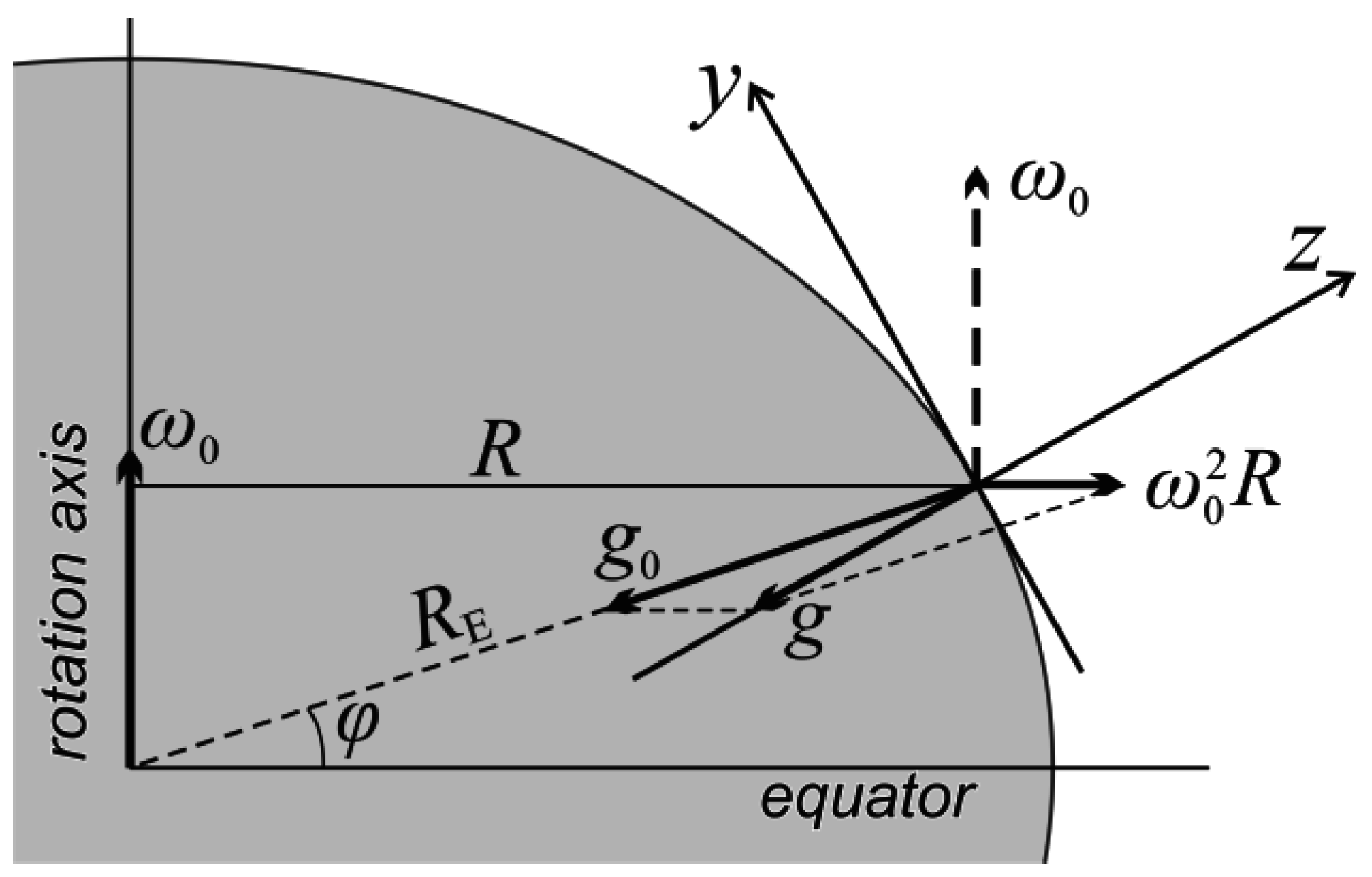
where g₀ is the gravity acceleration; $\nabla p$ the pressure gradient; 2[vω₀] the Coriolis acceleration; ${\omega }_0^{2}R$ the centrifugal acceleration; R the distance between the air parcel location and the rotation axis; f_fr the frictional force per unit mass; and ρ_i the density of moving air (in the static state, the density will be denoted as ρ_s). A system of coordinates is related to the Earth’s surface; abscissa axis (x-axis) is directed along the parallel; ordinate axis (y-axis) is directed along meridian; and applicate axis (z-axis) is perpendicular to the Earth’s surface (Figure 1). Equation (3) is Newton’s second law for the rotating Earth’s atmosphere.

In the atmosphere static condition, when v = 0, Equation (3) will have the form:

$$0=g_0-\frac{1}{{\rho }_{\mathrm{s}}}\nabla p_{\mathrm{s}}+{\omega }_0^{2}R$$

(4)

The static condition corresponds to the balance of the gravity force, the pressure gradient and the centrifugal force. It is more convenient to introduce the free fall acceleration vector equal to the gravity acceleration g₀ and centrifugal acceleration vectorial sum:

$$g=g_0+{\omega }_0^{2}R$$

(5)

Hence, the Earth’s geoidal surface is perpendicular to the free fall acceleration g.

Then, the atmosphere static state equation has the form:

$$0=g-\frac{1}{{\rho }_{\mathrm{s}}}\nabla p_{\mathrm{s}}$$

(6)

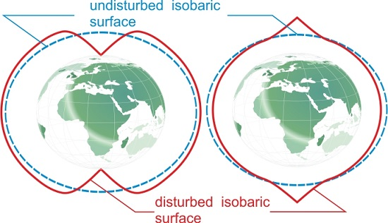
Under this form, the static state corresponds to the balance of the gravity force and the pressure gradient. In such notation, it follows from here that, in the static state, the isobaric surfaces are perpendicular to the free fall acceleration vector, i.e., parallel to the Earth’s geoidal surface. These isobaric surfaces are assumed as the atmosphere undisturbed state. Note that, in the static state, the undisturbed isobaric surface is usually approximated by a sphere [5,6,27,28,29]. Actually, the undisturbed isobaric surfaces are geoid-like. Thus, the static state is the basic state of the atmosphere in the so-called zero approximation. In this case, the baric and velocity fields are exactly determined.

At the steady motion dv/dt = 0, the isobaric surfaces of geoidal shape become disturbed; hence, the pressure may be written as [7]:

$$p=p_{\mathrm{s}}+p_{\mathrm{g}}$$

(7)

Similarly, the air density in Boussinesq approximation may be presented as [5,6]:

$${\rho }_{\mathrm{g}}={\rho }_{\mathrm{s}}\left(1-\alpha \Delta T\right)$$

(8)

where $\Delta T=T_{\mathrm{g}}-T_{\mathrm{s}}$ is the overheat function which is the air temperature disturbance relative to the static state: α = 1/T₀, T₀ = 273 K. The overheat function has a positive sign at warm air mass motion and a negative sign at cold air mass motion. The geostrophic state is the next basic state of the atmosphere in the so-called first approximation. In this case, the baric and velocity fields also should be determined exactly.

The equation of frictionless steady motion f_fr = 0 will have the following form:

$$\begin{gathered} 0=g-\frac{1}{{\rho }_{\mathrm{g}}}\nabla \left(p_s+p_{\mathrm{g}}\right)+2\left[v,{\omega }_0\right]\approx \\ -\frac{\alpha \Delta T}{{\rho }_{\mathrm{s}}}\nabla p_{\mathrm{s}}-\frac{1}{{\rho }_{\mathrm{s}}}\nabla p_g+2\left[v,{\omega }_0\right]=-\alpha \Delta Tg-\frac{1}{{\rho }_{\mathrm{s}}}\nabla p_{\mathrm{g}}+2\left[v,{\omega }_0\right] \end{gathered}$$

(9)

The geostrophic state of the atmosphere is determined by the balance of the gravity force, the pressure gradient and the Coriolis force. Here, we determined that, according to Equation (8), ${\rho }_{\mathrm{g}}\approx {\rho }_{\mathrm{s}}$.

The following expressions define the projections of the Earth rotation angular velocity [5,6,30]:

$${\omega }_{0x}=0,{\omega }_{0y}={\omega }_0\cos \phi ,{\omega }_{0z}={\omega }_0\sin \phi$$

(10)

Consider the projections of the stationary state motion Equation (9) in the coordinates system where the x-y-plane is tangent to geoid:

$$0=-\frac{1}{{\rho }_{\mathrm{s}}}\frac{\partial p_{\mathrm{g}}}{\partial x}+2v{\omega }_0\sin \phi -2w{\omega }_0\cos \phi$$

(11)

$$0=-\frac{1}{{\rho }_{\mathrm{s}}}\frac{\partial p_{\mathrm{g}}}{\partial y}-2u{\omega }_0\sin \phi$$

(12)

$$0=-\frac{1}{{\rho }_{\mathrm{s}}}\frac{\partial p_{\mathrm{g}}}{\partial z}+\alpha \Delta Tg+2u{\omega }_0\cos \phi$$

(13)

The free fall acceleration in the last equation equals $g=g_0-R_{\mathrm{E}}{\omega }_0^2{\cos }^2\phi$, where R_E is the Earth’s radius. The estimation of quantities shows that $R_{\mathrm{E}}{\omega }_0^2{\cos }^2\mathsf{\phi }\ll g_0$.

The third term in Equation (11) presents a product of the air velocity vertical component and the Earth’s angular velocity horizontal projection. Thus, one can conclude that there are two ways to obtain Equations (1) and (2): either by neglecting the vertical component of the air velocity, or by neglecting the horizontal projection of the Earth’s angular velocity. Although both assumptions lead to identical equations for the geostrophic wind projections, these assumptions are not equivalent. Within the geostrophic model of the atmosphere, on the basis of the scale analysis of variables involved in Equation (3) in the thin-layer approximation, it has usually been concluded that only the angular velocity component normal to the Earth’s surface is essential for the atmospheric dynamics. Thus, the third term in Equations (11) and (13) is usually neglected [5,6]. On the other hand, the importance of the Earth’s angular velocity horizontal projection for the atmospheric dynamics has been demonstrated in [9]. Thus, we can say that the geostrophic state of the atmosphere is a steady state at which the friction forces and the air velocity vertical component can be neglected. In such a situation, Equations (1) and (2) describing the geostrophic state of the atmosphere can be obtained. However, here we have the additional Equation (13) for the description of the geostrophic state. As a matter of fact, the goal of the present study is to reveal the novel aspects of the geostrophic state description resulting due to the accounting of Equation (13).

Thus, contrary to the usual definition of the geostrophic state, in our analysis, we use Equation (13). As a rule, the atmosphere static state equation appears as a third equation in the system describing the geostrophic state (see, e.g., [5,6]). This is due to the fact that the vertical projection of pressure gradient in Equation (13) is many orders of magnitude smaller than the Coriolis acceleration. However, from our point of view, it is incorrect to ignore Equation (13).

Due to the principal importance of this point, here we reconsider the scale analysis of the geostrophic state. Let us introduce the horizontal L and vertical H length scales such as $\delta =H/L\ll 1$. We have the following estimation of the Equation (11) components:

$$0~-\frac{p_{\mathrm{g}x}}{{\rho }_{\mathrm{s}}L}+2V{\omega }_0-2W{\omega }_0$$

(14)

The continuity equation leads to

$$\frac{V}{L}~\frac{W}{H},W~V\frac{H}{L}=\delta V$$

(15)

i.e., $W\ll V$. From here, we have

$$0~-\frac{p_{\mathrm{g}x}}{{\rho }_{\mathrm{s}}L}+2V{\omega }_0\left(1-\delta \right)$$

(16)

As it was noted in [6], to have the same order of magnitude of the horizontal pressure gradient and of the Coriolis acceleration, we must suppose that

$$p_{\mathrm{g}x}~2{\rho }_{\mathrm{s}}L{\omega }_{0}V$$

(17)

Thus, the third component of Equation (11) can be neglected as the component of lower order. Equation (12) gives the same order of magnitude for the pressure disturbance. The estimation of the vertical projection of the pressure gradient was made in [6] in the following way. Assuming that the disturbance of p_gz has the same order as the disturbance of p_gx (i.e., 2ρ_sLω₀V), it can be concluded that the ratio of the Coriolis acceleration and the vertical pressure gradient equals δ. Thus, the components of Equation (13) are of lower order than the components of Equations (11) and (12). For that reason, Equation (13) is ignored and the static state equation is used. However, how valid are the estimations presented above?

Suppose that the pressure disturbance has the form:

$$p_{\mathrm{g}}=p_{\mathrm{m}x}\sin \left(k_{x}x\right)+p_{\mathrm{m}y}\sin \left(k_{y}y\right)+p_{\mathrm{m}z}\sin \left(k_{z}z\right)$$

(18)

where k_xL = π, k_yL = π, k_zL = π. From Equations (11) and (12), it follows that

$$p_{\mathrm{m}x}~p_{\mathrm{m}y}~\frac{2{\rho }_{\mathrm{s}}LV{\omega }_0}{\pi }$$

(19)

and, from Equation (13), we have

$$p_{\mathrm{m}z}~\frac{2{\rho }_{\mathrm{s}}HV{\omega }_0}{\pi }$$

(20)

From here, it follows that $p_{\mathrm{m}z}\ll p_{\mathrm{m}x}, p_{\mathrm{m}y}$. However, if we suppose that the pressure disturbance has the form

$$p_{\mathrm{g}}=p_{\mathrm{m}}{e}^{-kz}\sin \left(k_{x}x+k_{y}y\right)$$

(21)

where k~1/L, then the vertical pressure gradient will have the same order of magnitude as the horizontal components. In other words, having no expression for the pressure disturbance, we cannot estimate the components of the pressure disturbance gradient.

Keeping in mind the discussion above, the systems (11)–(13) yield the geostrophic wind velocity horizontal projections:

$$u_{\mathrm{g}}=-\frac{1}{2{\omega }_0{\rho }_{\mathrm{s}}\sin \phi }\frac{\partial p_{\mathrm{g}}}{\partial y}$$

(22)

$$v_{\mathrm{g}}=\frac{1}{2{\omega }_0{\rho }_{\mathrm{s}}\sin \phi }\frac{\partial p_{\mathrm{g}}}{\partial x}$$

(23)

$$u_{\mathrm{g}}=\frac{1}{2{\omega }_0{\rho }_{\mathrm{s}}\cos \phi }\frac{\partial p_{\mathrm{g}}}{\partial z}-\frac{\alpha g}{2{\omega }_0\cos \phi }\Delta T$$

(24)

Taking the vector product of Equation (9) and the vector k, we get the expression for the geostrophic wind velocity:

$$v_{\mathrm{g}}=\frac{1}{2{\omega }_0{\rho }_{\mathrm{s}}\left(k,k_0\right)}\left[k,\nabla p_{\mathrm{g}}\right]$$

(25)

where k is the unit vector directed vertically up in the direction of z-axis perpendicular to the Earth’s geoidal surface; and k₀ the unit vector directed in the direction of the Earth rotation angular velocity. As is seen from Equation (25), the geostrophic wind is perpendicular to the pressure gradient and is directed along the isobaric surface.

As it was noted in [6], the isobaric surface disturbance cannot be determined within the geostrophic model, and a more general theory is required. However, as it will be demonstrated, some information about the shape of the disturbed isobaric surface can still be extracted from the analysis of the geostrophic wind.

Consider a special case when $\partial p_{\mathrm{g}}/\partial x=0$ and $-\partial p_{\mathrm{g}}/\partial y>0$. The pressure disturbance at steady motion will decrease along the y-axis from the equator to the pole (this is observed in the atmosphere on a global scale), and the geostrophic wind direction will be west to east, i.e., western flow will be observed in this case. It follows from Equations (22) and (24) that, for the initiation of warm air zonal eastward transport, the following condition must be satisfied:

$$\partial p_{\mathrm{g}}/\partial z>\alpha \Delta T{\rho }_{\mathrm{s}}g$$

(26)

and the pressure disturbance gradients must obey the relation:

$$\Delta T=\frac{1}{{\rho }_{\mathrm{s}}\alpha g}\cdot \left(\frac{\partial p_{\mathrm{g}}}{\partial z}+\mathrm{ctg}\phi \frac{\partial p_{\mathrm{g}}}{\partial y}\right)$$

(27)

It follows that for the existence of the zonal eastward transport of warm air, the vertical pressure disturbance gradient must be positive and greater than a certain value:

$$\frac{\partial p_{\mathrm{g}}}{\partial z}>-\mathrm{ctg}\phi \frac{\partial p_{\mathrm{g}}}{\partial y}, -\frac{\partial p_{\mathrm{s}}}{\partial y}>0$$

(28)

If this condition is not satisfied, then for the warm air mass, only east wind can be observed and the cold air mass will move in the eastward direction. The same result will take place if $\partial p_{\mathrm{g}}/\partial z\le 0$.

In other words, if we assume that the geostrophic state of the atmosphere corresponds to the isobaric surface of certain shape, which still needs to be determined, then at a given isobaric surface shape, the warm air will move westward (on condition that $\partial p_{\mathrm{g}}/\partial z\le 0$) and the cold air will move eastward (on condition that $\Delta T<\frac{1}{\alpha g{\rho }_{\mathrm{s}}}\partial p_{\mathrm{g}}/\partial z$).

3. Shape of the Disturbed Isobaric Surface

In the general case, it follows from Equations (22)–(24) that the pressure disturbance gradient $\nabla p_{\mathrm{s}}=\left(\partial p_{\mathrm{s}}/\partial x, \partial p_{\mathrm{s}}/\partial y, \partial p_{\mathrm{s}}/\partial z\right)$ has three nonzero components. Thus, if in the static state ($\nabla p_{\mathrm{s}}={\rho }_{\mathrm{s}}g$) the pressure gradient is directed along g, then in the general case of the geostrophic state at the arbitrary point of isobaric surface, the total pressure gradient

$$\nabla p=\nabla p_{\mathrm{s}}+\nabla p_{\mathrm{g}}$$

(29)

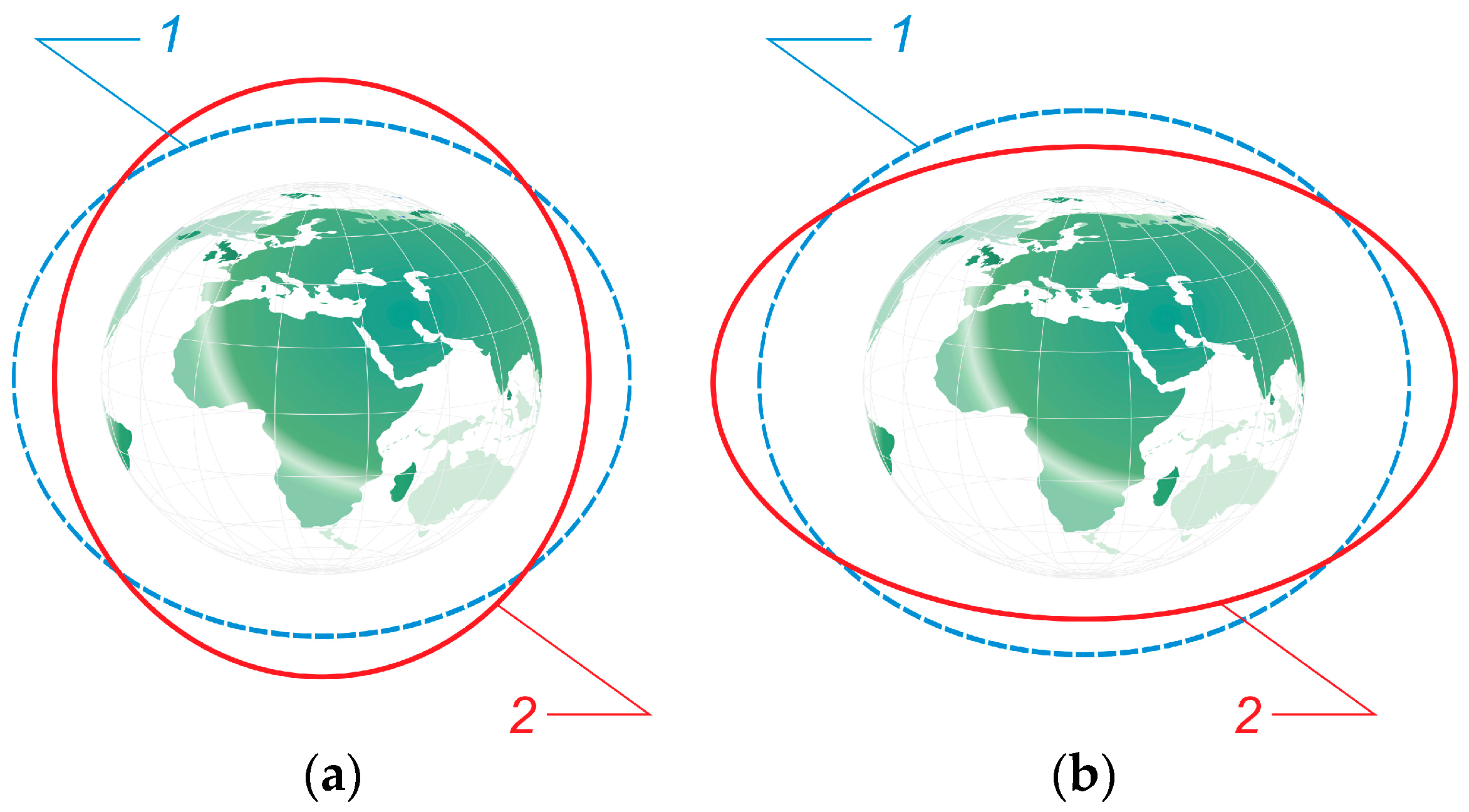
will be deflected from the g direction. In this case, contrary to the static state, the isobaric surface will not be perpendicular to g because it is perpendicular to $\nabla p$. Depending on the signs of components of the pressure disturbance gradient, the total pressure gradient can be deflected from g both towards the rotation axis and away from the rotation axis. In the first case, the isobaric surface will be extended along the Earth’s rotation axis in comparison with the isobaric surface in the static state (Figure 2a). Such a surface we will call the prolate geoid for short. In such a case, the pressure at the poles will be greater than the pressure in the static state. In the second case, the isobaric surface will be flattened at the poles along the Earth’s rotation axis in comparison with the isobaric surface in the static state (Figure 2b). Such a surface we will call the oblate geoid for short. In such a case, the pressure at the poles will be lower than the pressure in the static state.

The above reasoning is evidently inapplicable to the points at the equator and at the poles. Consider the points at the equator. It should be noted that, as sinφ = 0 at the equator, it has usually been concluded from Equations (22) and (23) that the geostrophic approximation does not work at the equator [6]. Actually, such a conclusion is unfounded if we do not know the disturbed isobaric surface. Supposing that the pressure gradient components are zero at the equator, we have the indefinite form (0/0). If we assume, for example, that p_g~cos²φ, then $\partial p_{\mathrm{g}}/\partial y~-2 cos\phi sin\phi$, and the indefinite form vanishes.

To address a question of the disturbed isobaric surface shape in the geostrophic state at the equator, consider the rectangular coordinate system shown in Figure 1 with the point of origin located at the equator. The vector Equation (9) is valid at any point. Neglecting the velocity vertical component, write the projections of Equation (9) onto the coordinate axes:

$$\partial p_{\mathrm{g}}/\partial x=0, \partial p_{\mathrm{g}}/\partial y=0$$

(30)

$$u_g=\frac{1}{2{\omega }_{0y}}\left(\frac{1}{{\rho }_{\mathrm{s}}}\frac{\partial p_{\mathrm{g}}}{\partial z}-g\alpha \Delta T\right)$$

(31)

Here, at the equator, ω_0y = ω₀ and the other components of the angular velocity are equal to zero. One can note that Equation (31) coincides with Equation (24); this fact additionally indicates the importance of Equation (24) for the analysis of the geostrophic state of the atmosphere. From Equations (30) and (31), it follows that $\nabla p$ is co-directional with $\nabla p_{\mathrm{s}}$. Thus, the isobaric surface is perpendicular to g at the equator, i.e., the isobaric surface is parallel to the geoidal isobaric surface of the static state. Equations (30) and (31) should be used at the equator instead of Equations (22)–(24). It follows from Equations (30) and (31) that the geostrophic wind velocity has only one component at the equator. This velocity component is directed along the equator. It follows from Equation (31) that this velocity component is positive if the following condition is satisfied:

$$\frac{\partial p_{\mathrm{g}}}{\partial z}>{\rho }_{\mathrm{s}}g\alpha \Delta T$$

(32)

If we assume that $\partial p_{\mathrm{g}}/\partial z=0$, then Equation (31) dictates that the warm air ($\Delta T>0$) will move to the negative direction (eastward), and cold air will move to the positive direction.

At any point infinitely near the equator, the meridional component of the velocity will also take place. From the continuity of motion, it can be concluded that the warm air starting from the equator goes along the spiral trajectory in the negative direction towards the pole. Analogously, the cold air will move from the equator in the positive direction along the spiral trajectory towards the pole. It should be noted that within the geostrophic model, the curved trajectory cannot be realized. However, we can consider the local direction of the geostrophic wind at each point.

Let us next analyze the disturbed isobaric surface shape at the poles. To this end, consider the rectangular coordinate system shown in Figure 1 with point of origin located at the pole (R = 0). If $\Delta T\ne 0$, the atmosphere motion equation at the pole will be

$$-\alpha \Delta T{g}_0-\frac{1}{{\rho }_{\mathrm{e}}}{\nabla p_{\mathrm{s}}|}_0+2\left[v_{\mathrm{g}}{\omega }_0\right]=0$$

(33)

Taking into account that 2[v_gω₀]_z = 0, the projections of this equation onto the coordinate axes have the form:

$$-\frac{1}{{\rho }_{\mathrm{s}}}{\frac{\partial p_{\mathrm{g}}}{\partial x}|}_0+2v_{\mathrm{g}}{\omega }_0=0$$

(34)

$$-\frac{1}{{\rho }_{\mathrm{s}}}{\frac{\partial p_{\mathrm{g}}}{\partial y}|}_0-2u_{\mathrm{g}}{\omega }_0=0$$

(35)

$$\alpha \Delta T{g}_0-\frac{1}{{\rho }_{\mathrm{s}}}\frac{\partial p_{\mathrm{g}}}{\partial z}=0$$

(36)

It can be seen that all three components of the pressure disturbance gradient $\nabla p_{\mathrm{g}}$ are nonzero, and the geostrophic wind velocity is also nonzero. Thus, in the geostrophic state, the total pressure gradient $\nabla p=\nabla p_s+\nabla p_g$ will be deflected from the g₀ direction. In this case, contrary to the static state ($\nabla p_{\mathrm{s}}={\rho }_{\mathrm{s}}{g}_0$), the isobaric surface will not be perpendicular to the rotation axis (or to g₀).

Consider the isobaric surface shape at the poles when overheat is equal to zero ($\Delta T=0$). As is seen from Equations (34) and (35), two cases are possible. In the first case, the geostrophic wind velocity is equal to zero at the pole. Then, the x- and y-components of the pressure disturbance gradient are equal to zero. In this case, we have the isobaric surface shape in the form of prolate or oblate geoids (Figure 2). In the second case, the geostrophic wind velocity is nonzero at the pole. Then, the x- and y-components of the pressure disturbance gradient are also nonzero. In this case, the pressure disturbance gradient vector $\nabla p_{\mathrm{g}}$ makes a right angle (π/2) with the static state pressure gradient vector $\nabla p_{\mathrm{s}}$. Hence, the resulting pressure gradient vector $\nabla p$ will be deflected from vertical (i.e., from $\nabla p_{\mathrm{s}}$). 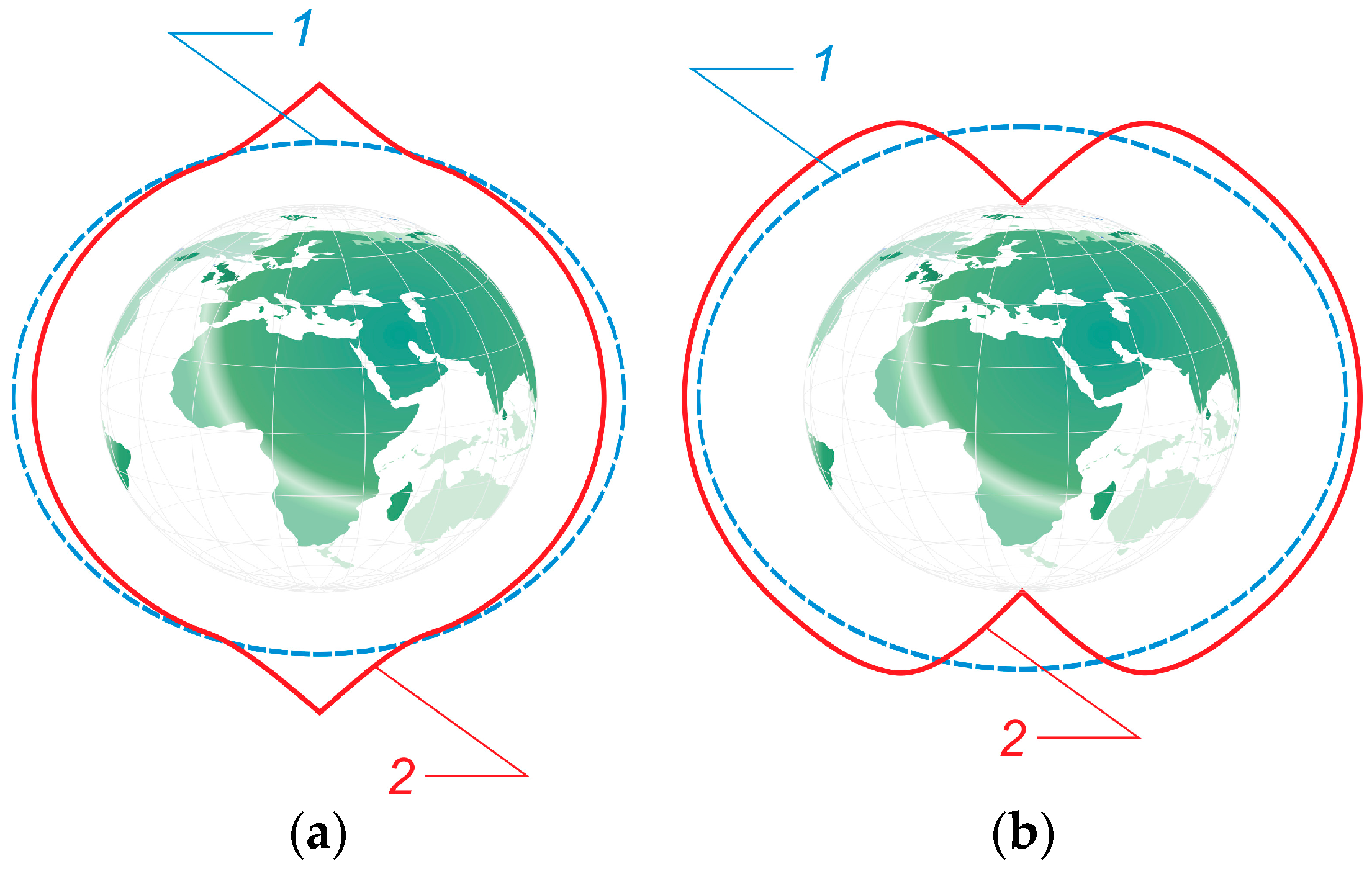This will lead to the disturbance of the isobaric surface at the pole. The isobaric surface will not be perpendicular to the rotation axis at the pole. The distinct conclusion about the type of the isobaric surface disturbance at the pole cannot be made on the basis of Equations (34)–(36). It is only clear that the pole is the exceptional point (in the sense of smoothness) of the function describing the isobaric surface. Then, the following scenarios are possible. The first scenario is the isobaric surface of an oblate geoid shape with local maxima or minima at the poles. The second scenario is the isobaric surface of a prolate geoid shape with local maxima or minima at the poles. However, if we assume that the baric minimum corresponds to the cyclonic motion, and baric maximum corresponds to the anticyclonic motion, then, as it follows from the continuity of motion, we must exclude the cases of oblate geoid with baric maxima at the poles and prolate geoid with baric minima at the poles. Thus, when the overheat at the equator is positive, the isobaric surface will have the prolate geoidal shape, and the warm air will move along the spiral towards the pole where the local maximum is taking place and the wind velocity has a finite value (Figure 3a). In this case, the polar vortex is of anticyclonic character. When the overheat at the equator is negative, the isobaric surface will have the oblate geoidal shape and the cold air will move along the spiral towards the pole where the local minimum is taking place and the wind velocity has a finite value (Figure 3b). In this case, the polar vortex is of cyclonic character.

Both described scenarios can exist simultaneously. The observations show that near the poles, the atmospheric circulation has the form of a westerly swirling near-surface vortex and an easterly swirling high-altitude vortex [31].

The observations show that the air temperature inside the polar vortex can be both higher and lower than the temperature of the surrounding atmosphere [10,13,16,17]. Consider the influence of the overheat sign on the isobaric surface disturbance at the pole. We start the analysis from the case of zero geostrophic wind velocity. At the positive values of the overheat ($\Delta T>0$), it follows from Equation (36) that the vertical component of the pressure disturbance gradient is positive $\partial p_{\mathrm{g}}/\partial z>0$ and directed oppositely to $\nabla p_{\mathrm{s}}$. Thus, the resulting pressure gradient decreases. Consider now the case of nonzero geostrophic wind velocity. At the negative values of the overheat, it follows from Equations (34)–(36) that the pressure disturbance gradient $\nabla p_{\mathrm{g}}$ makes an acute angle with the static state pressure gradient $\nabla p_{\mathrm{s}}$ (or with g₀) as the vertical component $\partial p_{\mathrm{g}}/\partial z$ is down-directed. Therefore, the resulting vector $\nabla p$ will be directed along the diagonal of the parallelogram made up of these two vectors. The deflection of the resulting vector $\nabla p$ from vertical (from $\nabla p_{\mathrm{s}}$) will be smaller than the deflection at zero overheat. It can be concluded that the isobaric surface has more flat minima at the poles. In other words, the negative overheat diminishes the pressure minimum depth at the pole. When the overheat value is positive, the angle between $\nabla p_{\mathrm{g}}$ and $\nabla p_{\mathrm{s}}$ will be greater than π/2. Therefore, in this case, the resulting vector $\nabla p$ will have a greater deflection from g₀ than that in the previous cases. In other words, the positive overheat elevates the pressure maximum at the pole.

These conclusions correlate with the research results described in [32]. According to [32], the polar vortex weakening is accompanied by the cold winters in mid-latitudes. In [32], it is asserted that the polar vortex weakening leads to the fall in temperature, namely, it induces a negative phase of Arctic Oscillation resulting in low temperatures in mid-latitudes. From our point of view, the opposite cause-and-effect relation is taking place. As it was shown, the steady geostrophic state with polar pressure extrema can exist. Any deviation from the geostrophic state leads to the ageostrophic oscillations. Particularly, negative phase of Arctic Oscillation leads to the polar vortex weakening.

The presented analysis does not give any preference to the appearance of either polar pressure maximum or polar pressure minimum; it only demonstrates the possibility of extrema of the pressure field at the poles in the geostrophic state. However, it should be noted that, at the poles, the pressure minima are usually observed and the air motion is of a cyclonic type [10,13,16,17].

Let us find the geostrophic wind divergence:

$$\begin{gathered} \frac{\partial u_{\mathrm{g}}}{\partial x}+\frac{\partial v_{\mathrm{g}}}{\partial y}=\frac{1}{2{\omega }_0}\left\{\frac{\partial }{\partial y}\left(\frac{1}{{\rho }_{\mathrm{g}}\sin \phi }\frac{\partial p_{\mathrm{g}}}{\partial x}\right)-\frac{\partial }{\partial x}\left(\frac{1}{{\rho }_{\mathrm{g}}\sin \phi }\frac{\partial p_{\mathrm{g}}}{\partial y}\right)\right\}= \\ -\frac{1}{2{\omega }_0{\rho }_{\mathrm{s}}\sin \phi }\left\{\frac{\partial p_{\mathrm{g}}}{\partial x}\left(\frac{1}{{\rho }_{\mathrm{s}}}\frac{\partial {\rho }_{\mathrm{g}}}{\partial y}+\mathrm{ctg}\phi \frac{\partial \phi }{\partial y}\right)-\frac{\partial p_{\mathrm{g}}}{\partial y}\left(\frac{1}{{\rho }_{\mathrm{s}}}\frac{\partial {\rho }_{\mathrm{g}}}{\partial x}+\mathrm{ctg}\phi \frac{\partial \phi }{\partial x}\right)\right\} \end{gathered}$$

(37)

As $\partial \phi /\partial x=0$, we have

$$\frac{\partial u_{\mathrm{g}}}{\partial x}+\frac{\partial v_{\mathrm{g}}}{\partial y}=-\frac{1}{2{\omega }_0{\rho }_{\mathrm{s}}\sin \phi }\left[\frac{\partial p_{\mathrm{g}}}{\partial x}\left(\frac{1}{{\rho }_{\mathrm{s}}}\frac{\partial {\rho }_{\mathrm{g}}}{\partial y}+\mathrm{ctg}\phi \frac{\partial \phi }{\partial y}\right)-\frac{1}{{\rho }_{\mathrm{s}}}\frac{\partial p_{\mathrm{g}}}{\partial y}\frac{\partial {\rho }_{\mathrm{g}}}{\partial x}\right]$$

(38)

From here, it follows that the divergence is nonzero in the geostrophic regime of the atmosphere:

$$\frac{\partial u_{\mathrm{g}}}{\partial x}+\frac{\partial v_{\mathrm{g}}}{\partial y}=-\frac{1}{2{\omega }_0{\rho }_{\mathrm{s}}\sin \phi }\left[\frac{\partial p_{\mathrm{g}}}{\partial x}\left(-\alpha \frac{\partial \Delta T}{\partial y}+\mathrm{ctg}\phi \frac{\partial \phi }{\partial y}\right)+\alpha \frac{\partial \Delta T}{\partial x}\frac{\partial p_{\mathrm{g}}}{\partial y}\right]\ne 0$$

(39)

Setting the divergence equal to zero, we find the condition at which this takes place:

$$\frac{\partial p_{\mathrm{g}}/\partial x}{\partial p_{\mathrm{g}}/\partial y}={\left(\frac{\mathrm{d}y}{\mathrm{d}x}\right)}_{\mathrm{g}}=\frac{\frac{\partial \ln {\rho }_{\mathrm{g}}}{\partial x}}{\frac{\partial \ln \left({\rho }_{\mathrm{g}}\sin \phi \right)}{\partial y}}=\frac{\alpha \frac{\partial \Delta T}{\partial x}}{\frac{\partial \ln \left({\rho }_{\mathrm{g}}\sin \phi \right)}{\partial y}}=0$$

(40)

It follows that the slope ratio of the tangent to the isobar and the parallel is determined by the horizontal gradients of air density (or by the gradients of the temperature disturbance) along the parallel and meridian. If the temperature does not change along the parallel, then (dy/dx)_g = 0. It follows that the geostrophic wind is directed along the parallel ($v_{\mathrm{g}}=0$) in this case. In the general case $\partial \Delta T/\partial x\ne 0,$ the geostrophic wind divergence is nonzero and both of the velocity components are also nonzero. It follows that the motion along the spiral from the equator towards the pole will take place.

The velocity divergence at the equator is

$$\frac{\partial u_{\mathrm{g}}}{\partial x}+\frac{\partial v_{\mathrm{g}}}{\partial y}=\frac{1}{2{\omega }_{0y}}\frac{\partial }{\partial x}\left(\frac{1}{{\rho }_g}\frac{\partial p_{\mathrm{g}}}{\partial z}-g\alpha \Delta T\right)=\frac{1}{2{\omega }_{0y}}\left[\frac{1}{{\rho }_{\mathrm{s}}}\frac{{\partial }^2{p}_{\mathrm{g}}}{\partial x\partial z}+\alpha \frac{\partial \Delta T}{\partial x}\left(\frac{1}{{\rho }_{\mathrm{s}}}\frac{\partial p_{\mathrm{g}}}{\partial z}-g\right)\right]=\frac{1}{2{\omega }_{0y}}\alpha \frac{\partial \Delta T}{\partial x}\left(\frac{1}{{\rho }_{\mathrm{s}}}\frac{\partial p_{\mathrm{g}}}{\partial z}-g\right)$$

(41)

It can be seen that the geostrophic wind divergence equals zero at the equator only if $\partial \Delta T/\partial x=0$. In general, the geostrophic wind divergence is nonzero at the equator, i.e., the airflow lines have a source at the equator. The velocity divergence at the pole is

$$\begin{gathered} \frac{\partial u_{\mathrm{g}}}{\partial x}+\frac{\partial v_{\mathrm{g}}}{\partial y}=-\frac{1}{2{\omega }_0}\left[\frac{\partial }{\partial x}\left(\frac{1}{{\rho }_{\mathrm{g}}}\frac{\partial p_{\mathrm{g}}}{\partial y}\right)-\frac{\partial }{\partial y}\left(\frac{1}{{\rho }_{\mathrm{g}}}\frac{\partial p_{\mathrm{g}}}{\partial x}\right)\right]= \\ -\frac{1}{2{\omega }_0}\left[\frac{\partial p_{\mathrm{g}}}{\partial y}\frac{\partial }{\partial x}\left(\frac{1}{{\rho }_{\mathrm{g}}}\right)-\frac{\partial p_{\mathrm{g}}}{\partial x}\frac{\partial }{\partial y}\left(\frac{1}{{\rho }_{\mathrm{g}}}\right)\right]=-\frac{\alpha }{2{\rho }_{\mathrm{s}}{\omega }_0}\left(\frac{\partial p_{\mathrm{g}}}{\partial y}\frac{\partial \Delta T}{\partial x}-\frac{\partial p_{\mathrm{g}}}{\partial x}\frac{\partial \Delta T}{\partial y}\right)= \\ -\frac{1}{2{\omega }_0}\left[\frac{\partial p_{\mathrm{g}}}{\partial y}\frac{\partial }{\partial x}\left(\frac{1}{{\rho }_{\mathrm{g}}}\right)-\frac{\partial p_{\mathrm{g}}}{\partial x}\frac{\partial }{\partial y}\left(\frac{1}{{\rho }_{\mathrm{g}}}\right)\right]=-\frac{\alpha }{2{\rho }_{\mathrm{s}}{\omega }_0}\left(\frac{\partial p_{\mathrm{g}}}{\partial y}\frac{\partial \Delta T}{\partial x}-\frac{\partial p_{\mathrm{g}}}{\partial x}\frac{\partial \Delta T}{\partial y}\right)= \\ \frac{\alpha }{2{\rho }_{\mathrm{s}}{\omega }_0}{\left[\mathrm{grad}{p}_{\mathrm{g}},\mathrm{grad}\Delta T\right]}_z \end{gathered}$$

(42)

It can be seen that the geostrophic wind divergence equals zero at the pole if either the velocity is zero or the pressure and temperature disturbance gradients are parallel to each other. In general, the geostrophic wind divergence is nonzero at the pole, i.e., the airflow lines have a sink at the pole.

Let us find the geostrophic wind vorticity at the equator:

$$\begin{gathered} {\mathsf{\Omega }}_{\mathrm{g}z}=\frac{\partial v_{\mathrm{g}}}{\partial x}-\frac{\partial u_{\mathrm{g}}}{\partial y}=-\frac{1}{2{\omega }_0}\frac{\partial }{\partial y}\left(\frac{1}{{\rho }_{\mathrm{g}}}\frac{\partial p_{\mathrm{g}}}{\partial z}-g\alpha \Delta T\right)= \\ -\frac{1}{2{\omega }_0}\left[\frac{1}{{\rho }_{\mathrm{s}}}\frac{{\partial }^2{p}_{\mathrm{g}}}{\partial y\partial z}+\alpha \frac{\partial \Delta T}{\partial y}\left(\frac{1}{{\rho }_{\mathrm{s}}}\frac{\partial p_{\mathrm{g}}}{\partial z}-g\right)\right]=-\frac{\alpha }{2{\omega }_0}\frac{\partial \Delta T}{\partial y}\left(\frac{1}{{\rho }_{\mathrm{s}}}\frac{\partial p_{\mathrm{g}}}{\partial z}-g\right) \end{gathered}$$

(43)

It is seen that the geostrophic wind vorticity is nonzero at the equator in the general case. The geostrophic wind vorticity at the pole is

$$\begin{gathered} {\mathsf{\Omega }}_{\mathrm{g}z}=\frac{\partial v_{\mathrm{g}}}{\partial x}-\frac{\partial u_{\mathrm{g}}}{\partial y}=\frac{1}{2{\omega }_0}\left[\frac{\partial }{\partial x}\left(\frac{1}{{\rho }_{\mathrm{g}}}\frac{\partial p_{\mathrm{g}}}{\partial x}\right)+\frac{\partial }{\partial y}\left(\frac{1}{{\rho }_{\mathrm{g}}}\frac{\partial p_{\mathrm{g}}}{\partial y}\right)\right]= \\ \frac{1}{2{\omega }_0}\left[\frac{1}{{\rho }_{\mathrm{s}}}\left(\frac{{\partial }^2{p}_{\mathrm{g}}}{\partial x^2}+\frac{{\partial }^2{p}_{\mathrm{g}}}{\partial y^2}\right)+\frac{\alpha }{{\rho }_{\mathrm{s}}}\frac{\partial p_{\mathrm{g}}}{\partial x}\frac{\partial \Delta T}{\partial x}+\frac{\alpha }{{\rho }_{\mathrm{s}}}\frac{\partial p_{\mathrm{g}}}{\partial y}\frac{\partial \Delta T}{\partial y}\right]= \\ \frac{1}{2{\rho }_{\mathrm{s}}{\omega }_0}\left[{\nabla }_{\perp }^2{p}_{\mathrm{g}}+\alpha \left({\nabla }_{\perp }{p}_{\mathrm{g}},{\nabla }_{\perp }\Delta T\right)\right] \end{gathered}$$

(44)

where ${\nabla }_{\perp }$ is the horizontal nabla operator. It is seen that the wind vorticity equals zero at the pole only if the velocity is zero. These results confirm the described picture and show that the air motion from the equator pointing towards the pole will take place along the spiral trajectory.

Thus, the presented discussion of the disturbed isobaric surface geometry demonstrates the existence of a pronounced persistent low- or high-pressure area near the poles. As follows from the analysis above, the polar vortices may be an inherent attribute of the geostrophic state of the atmosphere. In other words, the polar vortex corresponds to the basic state of the atmosphere, which can be disturbed by various factors such as the Arctic oscillations, the quasi biannual oscillations, the southern oscillations, El Niño, etc.

4. Conclusions

Thus, in the present work, it has been found that for the wind velocity projection onto the parallel, two equivalent expressions exist: the first demonstrates the velocity dependence on the pressure gradient along the parallel; and the second demonstrates the velocity dependence on the vertical pressure gradient. This result is obtained owing to the use of Equation (13), which has been traditionally neglected. When $\partial p_{\mathrm{s}}/\partial y<0$, for the existence of the zonal eastward transport of warm air, the vertical pressure disturbance gradient must be positive and greater than a certain value. Otherwise, for the warm air mass, only an east wind can be detected and the cold air mass will move in the eastward direction.

It has been demonstrated that the following alternative isobaric surface geometries are possible in the geostrophic state. The isobaric surface has a shape of an oblate or prolate geoid and the pressure at the pole is correspondingly lower or higher than the pressure in the static state. The geostrophic wind velocity, divergence and vorticity are equal to zero in these two cases. The prolate geoidal shape of the isobaric surface corresponds to the positive value of the overheating at the equator; and the oblate geoidal shape corresponds to the negative value of the overheating at the equator. The pressure minimum and maximum can occur at the poles in the mentioned cases of the oblate and prolate geoid. In such instances, the geostrophic wind velocity is nonzero at the poles. It follows from here that the polar vortexes can be a special feature of the geostrophic state of the atmosphere. However, the problem of mathematical definition of the exact shape of disturbed isobaric surface in the geostrophic state remains open. There is no doubt that, in addition to the geostrophic nature, various geophysical factors can influence the polar vortex formation process and complicate the resulting picture of the phenomenon.