1. Introduction
The planetary boundary layer (PBL) or atmospheric boundary layer refers to the part of the atmosphere that is directly influenced by the Earth’s surface and responds to surface forces within a timescale of an hour or less [
1,
2]. Because substances emitted into the PBL are gradually dispersed horizontally and vertically through the action of turbulence, if sufficient time elapses and there are no significant sinks, the PBL will become completely mixed; hence, the height of this layer is often called the mixing height. The mixing height (MH) is not only a key parameter for air pollution models, but is also an important parameter in the surface energy balance system (SEBS) for the estimation of turbulent heat flux. In the application of pollution models, the MH determines the volume available for the dispersion of pollutants and is involved in many predictive and diagnostic methods and/or models to assess pollutant concentrations [
3]. Similarly, evapotranspiration (ET) estimation models used for SEBS analysis require atmospheric data. Normally, these variables are estimated either from a large-scale meteorological model or from Obukhov similarity theory using data such as air pressure, temperature, humidity and wind speed at a reference height [
4].
Two basic possibilities for the practical determination of the MH are its derivation from profile data (measurements or numerical model output) and its parameterization using simple equations or models, which only need a few measured input values. The traditional approach uses the Parcel and Richardson number method to analyze the air temperature profile from radiosonde data [
3]. Currently, however, an increasing number of various remote sensing instruments and technologies are used to estimate MH. Compared with the free atmosphere, the MH has a much higher concentration of water vapor and aerosols. The abrupt decrease in water vapor and aerosols can cause a sharp Lidar signal change around the top of the boundary layer. Thus, Lidar can be used to monitor the temporal and spatial variations in the MH over urban and other areas [
5,
6,
7]. The use of SODAR, WTR and ceilometer instruments to estimate the MH has also been discussed extensively in the literature [
8]. These three instruments deliver five types of vertical profiles: wind and acoustic backscatter from the SODAR (Sound detection and ranging) instrument, wind, temperature and electromagnetic backscatter from the WTR (Wind-temperature-radar) instrument, and optical backscatter from the ceilometer. These can be combined to derive the MH [
9].
However, radiosondes, being launched only several times each day, with limited height resolution or routine ascents, do not provide continuous vertical profiles over time. Thus, it is difficult to study the time evolution of the MH [
3]. Furthermore, radiosonde data do not have good spatial representation since balloons released at one site drift with the wind. Since landuse is a crucial factor for MH evolution, this is a significant problem in urban areas, given their complex spatial variation in land use, as well as in basin-scale studies [
10]. Relying on ground-based remote sensing also limits the choice of the parameters that can be monitored. The classical models of turbulent transport in the atmospheric boundary layer require other input variables, such as wind speed, which are very difficult to measure accurately using land-based remote sensing tools. Hence, although the spatial structure of the MH is an important characteristic of the atmosphere, especially when the research area is at the basin-scale or larger, current methodologies cannot provide a clear indication of its spatio-temporal variation.
To date, only a few studies of limited scale have examined PBL processes using space-based remote sensing [
11]. However, as remote sensing has evolved, satellites providing atmospheric temperature and water-vapor profile data are increasingly available. Among them, MODIS has accumulated more than 10 years of global data (MOD07 and AIRS product). Some geostationary meteorology satellites, such as the Fengyun series, have a visitation frequency of half an hour [
12], but their vertical resolution is limited. If space-based remote sensing data can detect the abrupt decrease of water vapor at the top of the PBL, and thus diagnose the MH, it will alleviate the lack of detailed spatio-temporal information for the MH.
The basic advantages of space-based systems are their continuous operation and the absence of any impact on the investigated flow. The objective of the present study is to develop a method for estimating a high spatial-resolution MH and associated variables as input for a 1-km resolution SEBS model for the Heihe River Basin using only atmospheric variables from space-based remote sensing platforms without any reliance on ground measurements. For the future, we hope our results, when combined with other similar spaced-based data, can provide a global data set for the application of pollutant models and evapotranspiration estimation models.
In this paper,
Section 2 contains the introduction of the study area and data;
Section 3 contains the method of processing radiosonde data for the validation of the MH, the gap filling of the MODIS profile data and the main retrieval method of the MH;
Section 4 is comprised of the results from
Section 3 and some validation; and
Section 5 and
Section 6 contains the discussion and results of the paper.
2. Study Area and Data
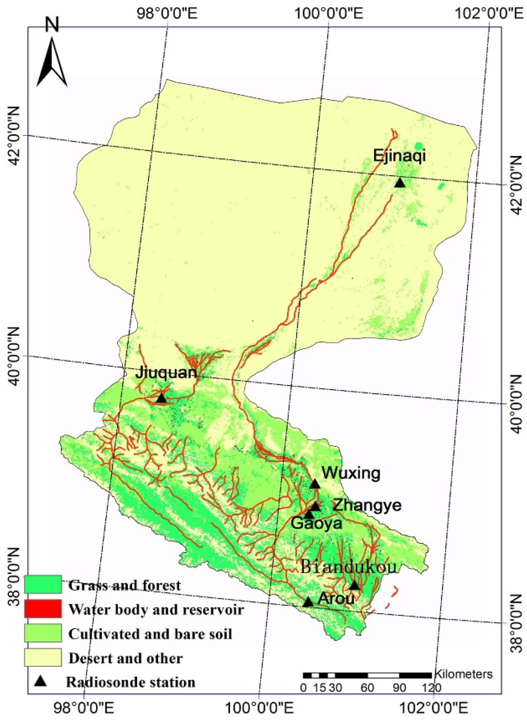
The Heihe river basin (HRB) is a typical arid region of north western China (
Figure 1). It is located between 96°42′–102°00′E and 37°41′–42°42′N with a drainage area of 130,000 km
2, and has a desert-oasis-river landscape structure [
13]. It is an ideal field laboratory to pursue integrated PBL studies for several reasons. Firstly, although human activity, especially urban heat islands and skyscrapers, can have a large impact on the structure of the PBL, the economy here is relatively backward and there are few metropolises, so any effect is limited. Additionally, comprehensive experiments with radiosonde observations, such as WATER [
14] and HiWATER [
15] have been conducted here, and radiosondes have been released at Wuxing, Gaoya, Biandukou and Arou. Further, three national radiosonde stations in the region (at Zhangye, Jiuquan, and Ejinaqi) have accumulated standard sounding data for more than 20 years (
Figure 1).
Radiosondes are the most common source of data for operational determination of the MH. They are widely distributed spatially, and the data are subjected to quality control on a continual basis. The three national stations Zhangye, Jiuquan and Ejinaqi within the HRB, operated by the China Meteorological Administration, launch radiosondes twice daily at 08 Beijing Time (BJT = UTC/GMT + 8 hours), and 20 BJT. These standard sounding data include regular pressure layers (1000, 920, 850, 700, 500, 400, 300, 250, 200 hPa, etc.) and were obtained through the Natural Science Foundation of China (NSFC). High vertical resolution sounding data for 2008 and 2012 were obtained from the WATER and HiWATER projects, respectively, which collected GPS-located radiosonde sounding observations for the middle and upper stream sections of the HRB. Both sets of sounding data were used for validation.
The MODIS MOD07 L2 product was chosen as our primary data source for deriving the MH, mainly because of its high spatial resolution and the advancement of its data collection process. Although the MODIS is not a sounding instrument, it does have many of the spectral bands found on the High Resolution Infrared Radiation Sounder (HIRS) currently in service on the polar orbiting NOAA TIROS Operational Vertical Sounder (TOVS). Thus, it is possible to generate the vertical profiles of temperature and moisture as well as total column estimates of precipitable water vapor. The MODIS algorithms were adapted from the operational HIRS and GOES algorithms, with adjustments to accommodate the absence of stratospheric sounding spectral bands and to realize the advantage of greatly increased spatial resolution (1 km MODIS
vs. 17 km HIRS) with good radiometric signal to noise ratio (better than 0.35 C for typical scene temperatures in all spectral bands) [
16]. MODIS MOD07 atmosphere profile data include 20 specific pressure layers; each layer contains elevation, air temperature and dewpoint temperature information. The air pressure layers from the surface to upper air are at 1000, 950, 920, 850, 780, 700, 620, 500, 400, 300, 250, 200, 150, 100, 70, 50, 30, 20, 10 and 5 hPa. For most situations, the MH is at an elevation below 600 hPa; therefore, our analysis emphasizes the data from 600 hPa to 1000 hPa.
Figure 1.
Heihe river basin location and landuse; location of radiosonde stations.
Figure 1.
Heihe river basin location and landuse; location of radiosonde stations.
3. Methodology
3.1. In Situ Radiosonde Data Processing
The most common method to determine the MH from radiosonde data is based on the Richardson number method, but it is usually used under convective conditions. The Richardson number
Rib is defined as [
1]:
where
g is the gravity acceleration,
z0 is the altitude of the measurement location above sea level,
θ is the potential temperature, and
μ(
z) and
v(
z) the wind zonal and meridional components, respectively. The MH is defined as the height where the Richardson number equals the critical Richardson number of 0.21 [
17,
18]. At heights where
Rib is higher than the critical value, the atmosphere is considered to be free of turbulence (free troposphere). Unfortunately, the MH estimates based on standard radiosonde data can result in quite high uncertainty [
19,
20]. Particular problems occur under stable atmospheric conditions since no universal relationships seem to exist between the profiles of temperature, humidity or wind. Consequently, other methods must be used in combination [
21,
22]:
- (1)
The height at which the virtual potential temperature matches the surface value;
- (2)
The level of the maximum vertical potential temperature gradient;
- (3)
The base of an elevated temperature inversion.
In our paper, the Richardson number method is used to define the radiosonde MH under convective conditions and the combination method is used under stable conditions.
3.2. MODIS Data Processing
The satellite data suffer from data gaps. Some gaps are internal to the satellite, primarily related to its orbits or to instrument failures, while others are external such as cloud contamination [
23]. Several solutions have emerged in recent years [
24]. In the HRB, the presence of cloud cover is the main factor resulting in spatial gaps in the data. In order to provide complete spatial coverage, gap-filling methodology was devised, which has both spatial and temporal components. First, the spatial component investigates a 5 × 5 pixel area. If enough data are available (more than half of the total), the inverse distance weighted average method is used to fill the empty pixel; alternatively the window is expanded to 10 × 10. The expansion process is repeated until a specified maximum window size (usually, 15 × 15 pixels) is reached. Within the maximum window, if there is still too little available data (less than half of the total), then the average value at the same location from the most recent clear day before and after is substituted.
In addition to the primary air temperature and dewpoint temperature profiles, other variables were also derived, including saturation vapor pressure, actual vapor pressure, relative humidity, mixing ratio of water vapor, and virtual potential temperatures, using the conversion equations defined by the Food and Agriculture Organization (FAO) of the United Nations [
25].
3.3. MH Retrieval
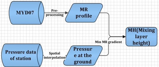
Under clear conditions within the entrainment zone, turbulent boundary layer eddies mix aerosol and water vapor-laden air with cleaner free tropospheric air. This mixture of clear and dirty air together in the entrainment zone prevents aerosols and water vapor mixing with free air. Thus, other researchers have suggested several methods to retrieve the MH based on the assumption that water vapor and aerosols are much more abundant within the PBL than in the free troposphere above it [
26]. After examining the ability of all the primary and conserved variables (
Figure 2) to identify MH, only the mixing ratio of the water vapor (MR) profile was able to provide evidence of the MH in the Heihe river basin: There was an abrupt decrease for MR profile. Accordingly, an automated method based on the level of the minimum vertical gradient of the MR profile was proposed for identifying the MH.
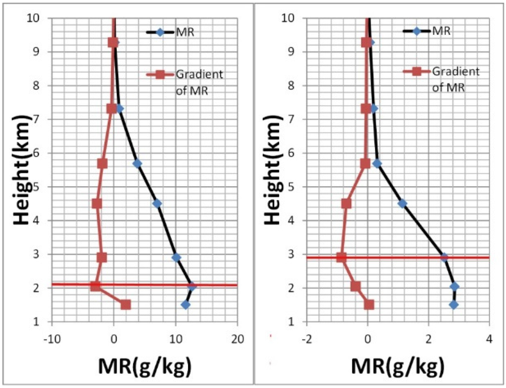
As an example,
Figure 3 shows two profiles of vertical MR gradients on 10 August 2012, for Jiuquan and Zhangye. The height of the minimum vertical gradient of the MR is coincident with an abrupt decrease in the MR and can be considered as the top of the mixed layer. Based on this, the height (location) of the MH is retrieved pixel by pixel.
Figure 2.
Profile of primary and conserved variables retrieved from MODIS atmospheric profile data for Jiuquan and Zhangye radiosonde stations on 10 August 2012.
Figure 2.
Profile of primary and conserved variables retrieved from MODIS atmospheric profile data for Jiuquan and Zhangye radiosonde stations on 10 August 2012.
Figure 3.
Profile of the MR and vertical gradient of the MR (in red) retrieved from MODIS atmospheric profile data for Jiuquan and Zhangye radiosonde stations on 10 August 2012.
Figure 3.
Profile of the MR and vertical gradient of the MR (in red) retrieved from MODIS atmospheric profile data for Jiuquan and Zhangye radiosonde stations on 10 August 2012.
4. Results and Validation
4.1. Radiosonde Data
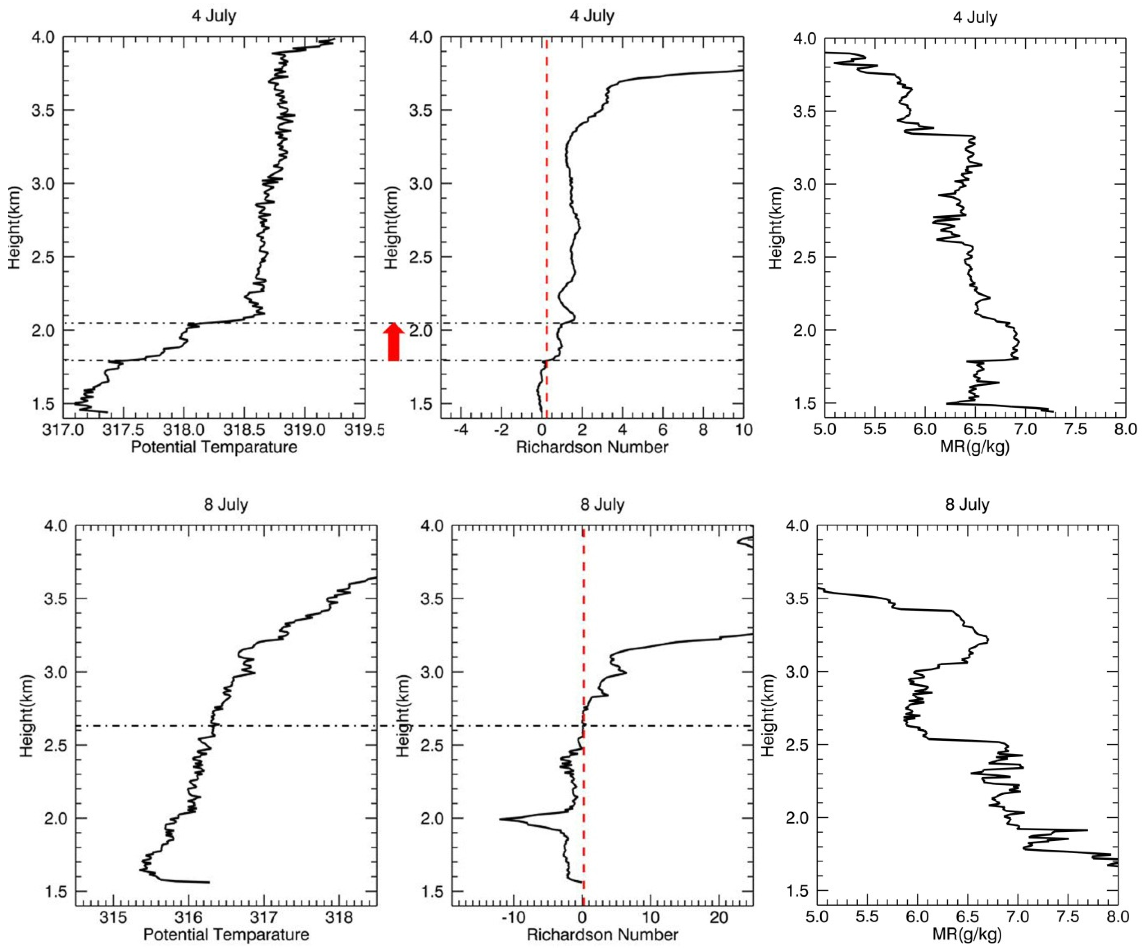
4 July and 8 July 2012 were used for analysis of the
in situ radiosonde data from the HIWATER project. Because of different air conditions on these days, different methods were used for each day. Although we lack direct observations of the convection and buoyancy flux, we can infer the stability of air conditions from the structure of the potential temperature profile [
1]. 4 July was stable and 8 July was convective. In
Figure 4, the vertical dashed line represents
Rib = 0.21, and the horizontal dashed line indicates the height of the MH. In the upper figure, there two dashed lines; the lower one is the height of
Rib = 0.21, and the upper one is the level of the maximum vertical potential temperature gradient. For 4 July, the height of the stable boundary layer was identified as the level of the maximum vertical potential temperature gradient instead of the height where the Richardson number equaled 0.21, as shown in
Figure 4. For 8 July, the height of the convection boundary layer was identified using the Richardson number method,
i.e., as the height where the Richardson number equals its critical value of 0.21 (
Figure 4, lower panels). On both days, there was an abrupt decrease in the MR at the height of the MH, which justifies our method of using the MR to derive the MH from MODIS profile data (
Figure 4).
Figure 4.
Profile of potential temperature, MR and Richardson number calculated from radiosonde data collected at Gaoya station on 4 July and Wuxing station on 8 July, 2012.
Figure 4.
Profile of potential temperature, MR and Richardson number calculated from radiosonde data collected at Gaoya station on 4 July and Wuxing station on 8 July, 2012.
4.2. MODIS Data Processing
As previously discussed, there were missing data in the MODIS atmospheric profiles due mainly to cloud coverage. A spatial-based gap-filling method was used for continuity when the missing data were limited. Where large areas were missing, data from the most recent available clear day were substituted (
Figure 5).
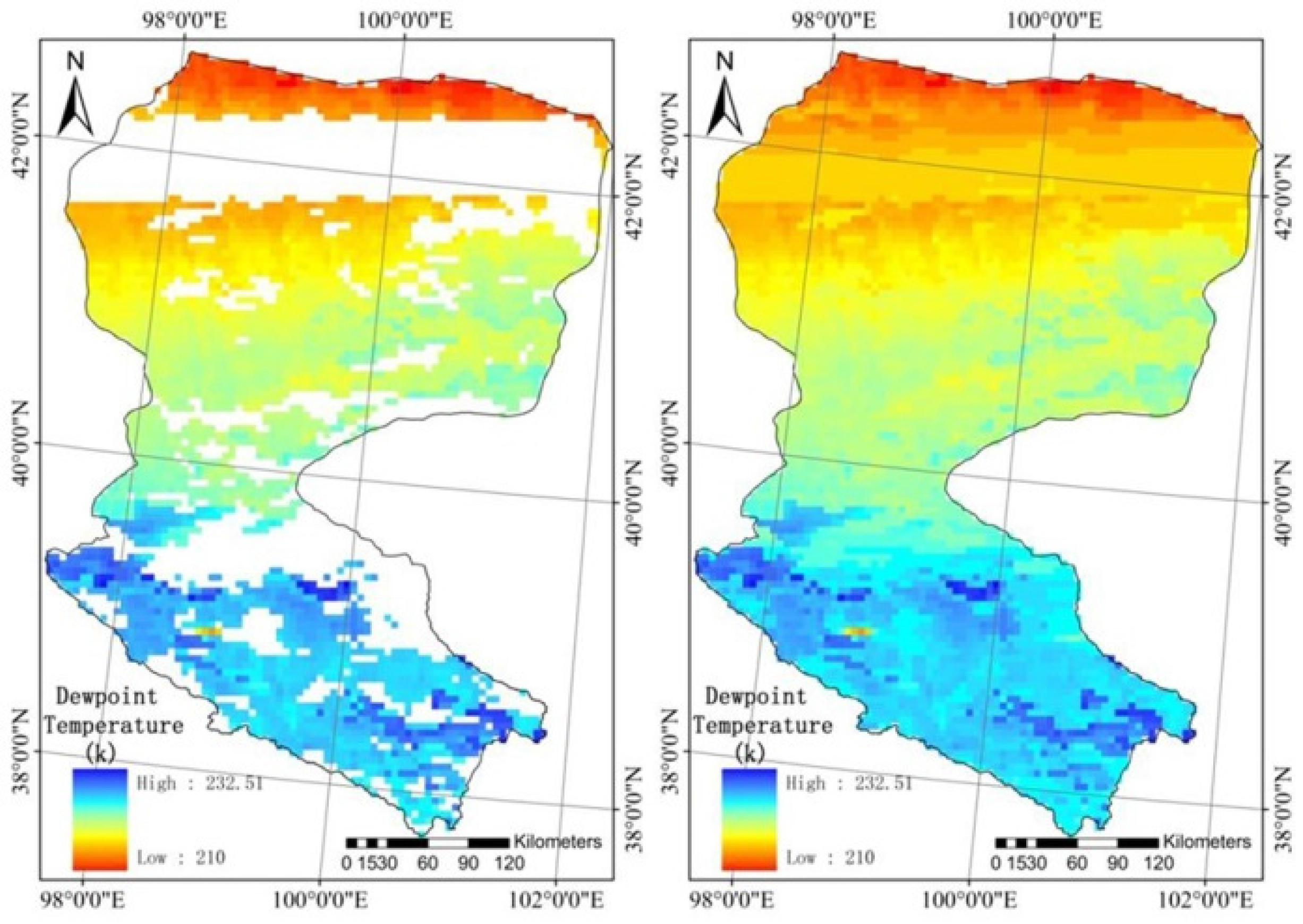
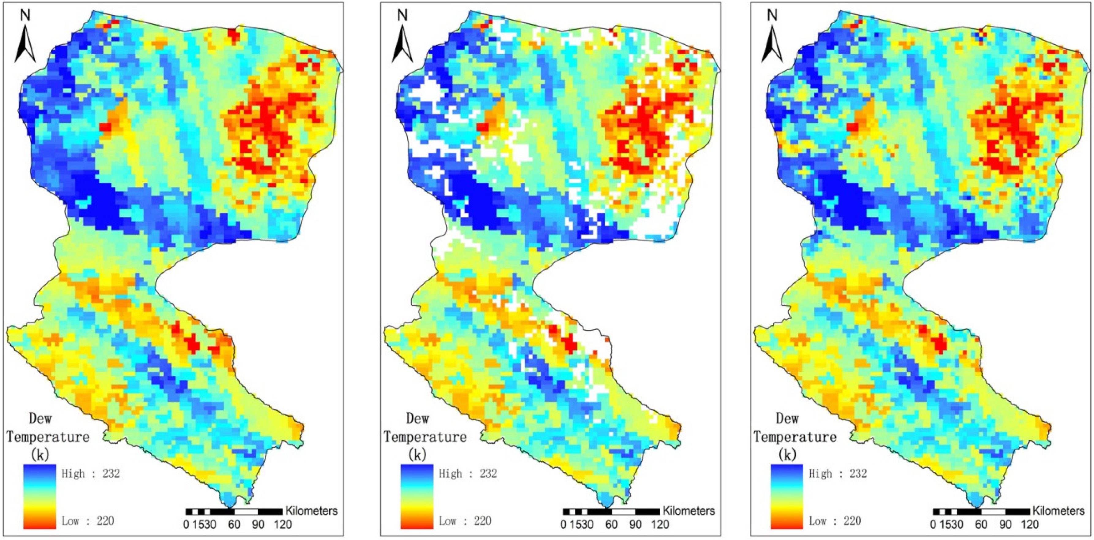
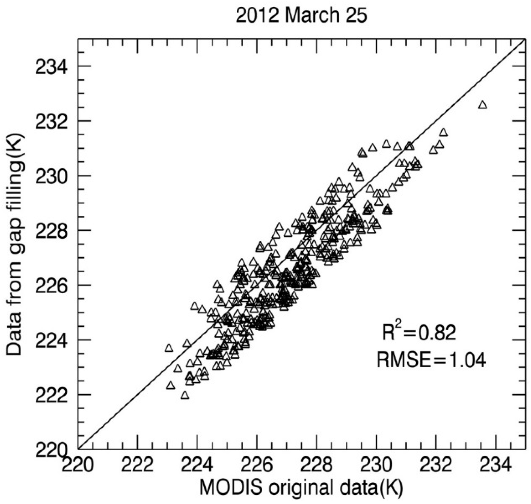
The gap filling and its impact were assessed by using a situation where all MODIS data were available. Using 25 March 2012 as an example, certain areas were screened out randomly, and gap filling was performed for these areas. Then, the gap-filled data were compared to the original data on a pixel basis. As shown in
Figure 6, the left picture is the original MODIS dewpoint temperature data from a clear sky, the middle one is the MODIS dewpoint temperature data after screening some areas, and the right picture is gap-filled from the middle one. From
Figure 6 and
Figure 7, it is clear that our gap filling method worked well when the area of missing data was limited and data from the most recent available clear day were used. The coefficient of determination (R
2) was 0.82 and the RMSE was 1.04 for the original and gap-filled data; if large missing areas were considered, a poorer relationship was obtained: the coefficient of determination (R
2) was 0.31 and the RMSE was 2.13. The moisture structure of the boundary layer has large spatial variations and can be totally different between cloudy and cloud-free conditions and between different days. Therefore, it is not a good idea to fill sections with large gaps. In particular, using the average value from the most recent clear day in the gap-filling process will produce problematic and unrealistic spatial changes of moisture data. Thus, we prefer gap filling using data from areas with few missing values and avoiding areas with extensive missing data.
Figure 5.
The moisture data for the Heihe river basin at 700 hPa before and after application of the gap-filling process for 2 January 2012.
Figure 5.
The moisture data for the Heihe river basin at 700 hPa before and after application of the gap-filling process for 2 January 2012.
Figure 6.
The validation of moisture data for the Heihe river basin at 700 hPa: original data, screening area and data after gap filling for 25 March 2012.
Figure 6.
The validation of moisture data for the Heihe river basin at 700 hPa: original data, screening area and data after gap filling for 25 March 2012.
Figure 7.
MODIS original moisture data vs. those from the gap-filling method for 25 March 2012 at 700 hPa pressure within the Heihe River Basin.
Figure 7.
MODIS original moisture data vs. those from the gap-filling method for 25 March 2012 at 700 hPa pressure within the Heihe River Basin.
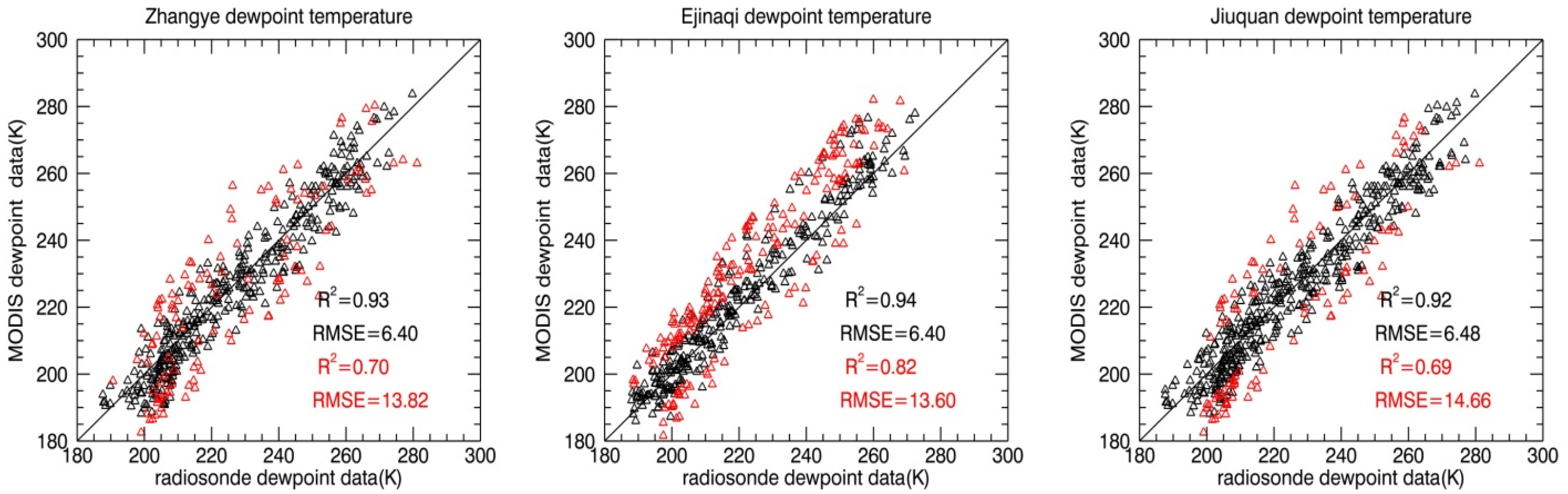
After gap filling, comparisons between the temperature and dewpoint temperature profiles from
in situ radiosonde data and those from MODIS MYD07 for the Heihe river basin under clear and cloudy sky conditions showed a strong correlation. In
Figure 8, validation of the MODIS data from clear and cloudy sky conditions is indicated in black and red colors, respectively. The coefficient of determination (R
2) between the satellite-retrieved moisture profiles and the
in situ measured temperature profiles of the black points for the Zhangye, Jiuquan, and Ejinaqi stations during 2012 for each regular pressure layer is 0.93, 0.94 and 0.92, respectively. This indicates that the MODIS atmospheric profile data correlate well with measured moisture profiles from the radiosondes. The RMSE for the dewpoint temperature is approximately 6.5 K and 0.6 g/kg for the MR. Compared with clear sky, the data from gap filling under cloudy sky conditions indicate a weaker correlation; as shown in
Figure 8, the R
2 and RMSE for the three stations are 0.70, 0.82, 0.69 and 13.82, 13.60, 14.66, respectively. These errors may partially be a consequence of the difference between the radiosonde sending time (8 and 20 BJT) and the satellite overpass time (about 13-15 BJT), arising mainly from the uncertainty originating from the gap filling method.
Figure 8.
Validation between MODIS moisture data and radiosonde data for 2012 at Zhangye, Jiuquan and Ejinaqi stations for regular pressure layers.
Figure 8.
Validation between MODIS moisture data and radiosonde data for 2012 at Zhangye, Jiuquan and Ejinaqi stations for regular pressure layers.
4.3. MH Validation
Most of the optical-thermal satellites, including the two MODIS satellites (Terra and Aqua), have overpass times ranging from 9:00 to 15:00 local time. The greatest depth of the PBL usually occurs in the afternoon between 13:00 and 17:00 local time. This most closely corresponds to Aqua’s overpass time (13:00–15:00); therefore, MODIS MOD07 data from Aqua were used.
Table 1 compares MH estimates from
in situ radiosonde data to those from the MODIS data on selected days in 2008 and 2012 when the radiosonde balloon release time was close to the satellite overpass time. The data in
Table 1 indicate that the MH calculated from MODIS is largely coincident with that from
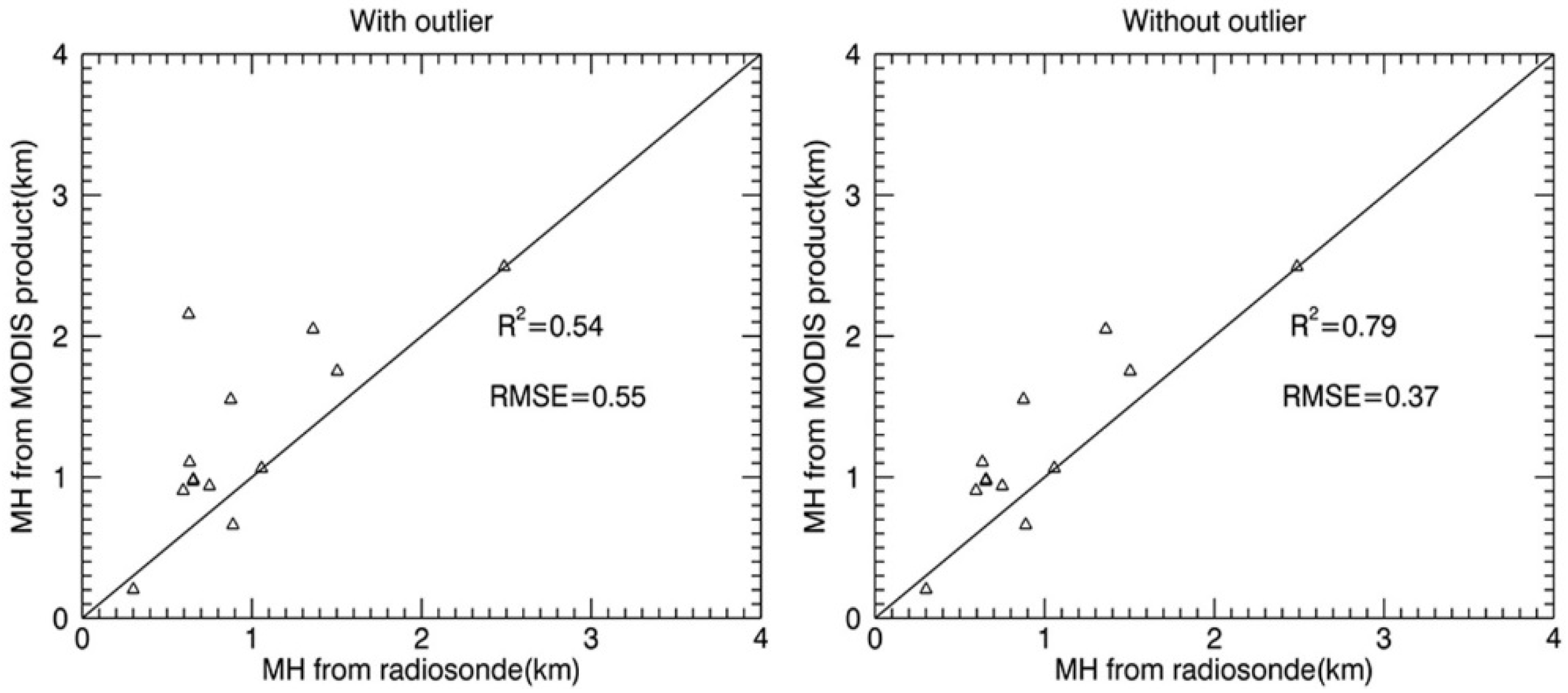
in situ radiosondes. The absolute error is below 500 meters, which is the resolution of the MODIS moisture profile at its base. However, there is a significant error for 4 July. As discussed previously and demonstrated in
Figure 4, the potential temperature profile for 4 July suggests stable atmospheric conditions. For our method, determination of the MH from the MODIS profile data under stable conditions can result in substantial error. This appears to be the case for 4 July. Unfortunately, the lack of
in situ data under stable air conditions, which would enable additional comparisons, inhibits further verification of our speculation. The assumption that stable air conditions may cause substantial errors needs further examination. The effect of this error is apparent from
Figure 9. By omitting the data for 4 July, the R
2 between the two estimations increases from 0.59 to 0.82, the RMSE decreases from 550 m to 370 m and relative error changes from 44% to 28%.
Table 1.
Comparison between the MH calculated from radiosonde data and that from MODIS data for 13 days in 2008 and 2012 for the Heihe river basin.
Table 1.
Comparison between the MH calculated from radiosonde data and that from MODIS data for 13 days in 2008 and 2012 for the Heihe river basin.
| Number | Date | Released Time (BJT) | MODIS overpass Time (BJT) | Place | MH from Radiosonde (m) | MH from MODIS (m) | Relative Error |
|---|
| 1 | 2008/3/15 | 11:10 | 13:15 | Arou | 301 | 203 | -0.326 |
| 2 | 2008/3/17 | 11:46 | 14:40 | Biandukou | 888 | 661 | -0.256 |
| 3 | 2008/4/1 | 11:15 | 13:55 | Arou | 653 | 971 | 0.487 |
| 4 | 2008/7/5 | 12:14 | 13:15 | Biandukou | 633 | 1106 | 0.747 |
| 5 | 2012/6/29 | 14:26 | 14:10 | Wuxing | 750 | 937 | 0.249 |
| 6 | 2012/7/3 | 11:57 | 13:45 | Gaoya | 2487 | 2492 | 0.002 |
| 7 | 2012/7/4 | 14:09 | 14:30 | Gaoya | 627 | 2156 | 2.439 |
| 8 | 2012/7/5 | 11:07 | 13:30 | Wuxing | 595 | 905 | 0.521 |
| 9 | 2012/7/7 | 13:47 | 13:20 | Wuxing | 1503 | 1752 | 0.166 |
| 10 | 2012/7/8 | 13:49 | 14:00 | Wuxing | 1057 | 1062 | 0.005 |
| 11 | 2012/7/10 | 14:45 | 13:50 | Wuxing | 1360 | 2049 | 0.507 |
| 12 | 2012/8/1 | 13:38 | 13:15 | Arou | 875 | 1551 | 0.773 |
| 13 | 2012/8/2 | 13:55 | 13:55 | Wuxing | 655 | 983 | 0.501 |
If there is a regular diurnal cycle of the MH in the Heihe river basin, the residual layer of boundary layer will also be moist and it is likely that the top of the residual layer instead the top of the actual ABL will be found. Therefore, from
Table 1 we can find that most of the daily MH values from MODIS data are larger than those from radiosonde data.
Figure 9.
R2 and RMSE for the MH values retrieved using our method and radiosonde data for all days (a) and for convective days (b) at the Heihe river basin in 2008 and 2012.
Figure 9.
R2 and RMSE for the MH values retrieved using our method and radiosonde data for all days (a) and for convective days (b) at the Heihe river basin in 2008 and 2012.
4.4. MH Spatial and Temporal Patterns
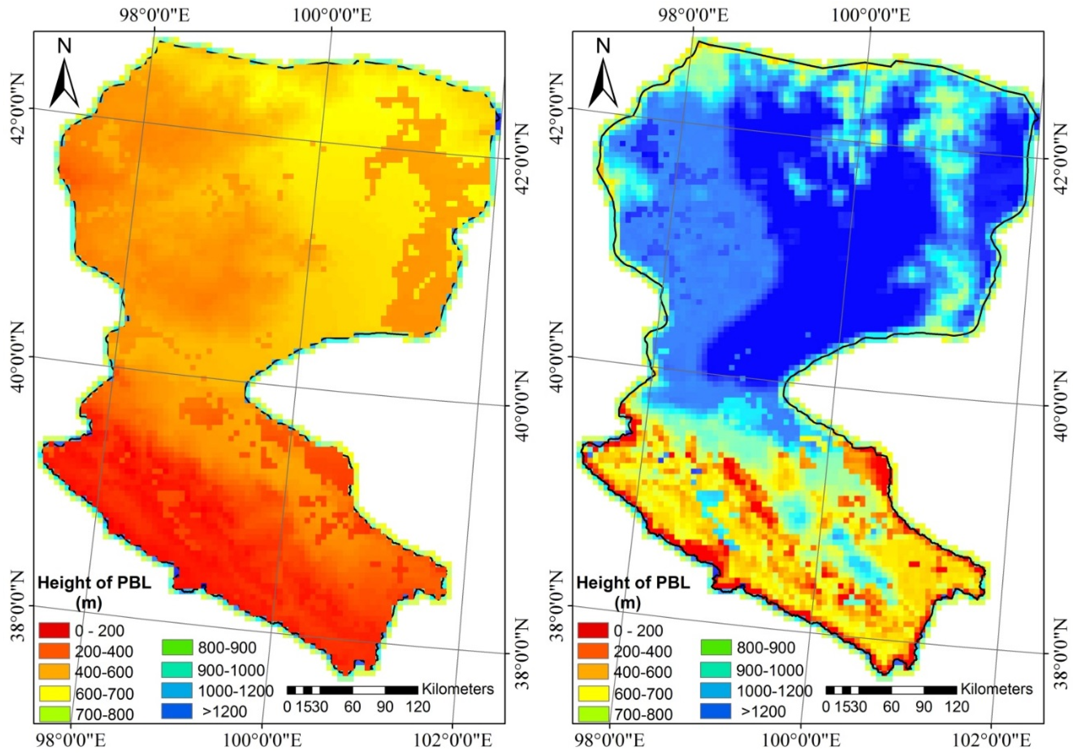
After data pre-processing and model calculation, the peak MH for each day was calculated for selected days in 2008 and 2012. The results from clear days in winter and summer are mapped in
Figure 10 for two example days.
Figure 10.
Spatial variation of the MH derived from the MODIS MOD07 product for the clear days 8 January and 6 July 2012.
Figure 10.
Spatial variation of the MH derived from the MODIS MOD07 product for the clear days 8 January and 6 July 2012.
The mixing layer height is primarily driven by variation in the vertical flux of energy and momentum caused by the balance between the heating of the earth’s surface by incoming solar radiation and radiative cooling of the surface [
27,
28,
29]. Accordingly, as
Figure 10 shows, the MH is lower in the winter and relatively higher in the summer, demonstrating that net radiation is the main factor driving the development of the PBL. Especially in the western portion of the downstream area, where desert land use dominates, the growth amount of the MH extends higher than that in the middle and upper stream regions where oasis landscapes occur. Forest and grass vegetation may have a buffer for temperature variation; therefore, the oases area results in more consistent land surface temperatures, which keeps sensitive heat more stable and lower than in the desert area, eventually leading to a similarly stable and lower change in the MH. For every single day, the MH showed a stronger correlation with the actual land conditions,
i.e., higher for desert than grass/forest during both winter and summer.
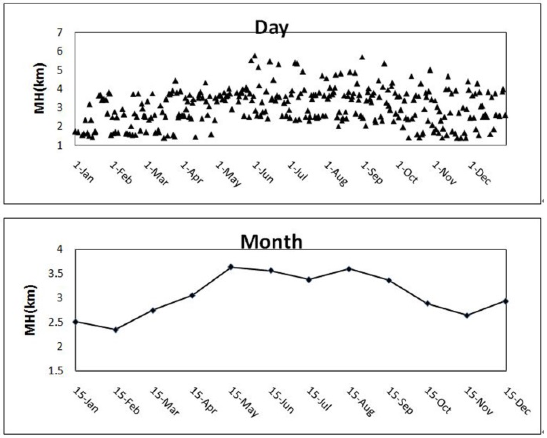
The annual variation in the MH was analyzed at the Gaoya station.
Figure 11 shows the daily variation and monthly average MH at this station in 2012. There is a clear annual cycle with the MH growing from about 2500 meters in January to 3000–3500 meters in the summer and autumn, and descending to about 2500 meters again at the end of the year.
Figure 11.
Daily and monthly variation in the MH calculated from the MODIS profile data from the Gaoya station in 2012.
Figure 11.
Daily and monthly variation in the MH calculated from the MODIS profile data from the Gaoya station in 2012.
5. Discussion
Although the average trend of the MH is reasonable at the Gaoya station, there is a large variation from day to day. Several reasons may account for this daily variation: the MH is strongly related to net radiation, which has a large daily variation; there is a difference between the overpass times of the satellite on each day, and the diurnal variation of the MH can be as much as several kilometers; the presence of cloud cover, and the consequent use of gap-filling to estimate missing data may generate large errors in the moisture profile; under stable air conditions in particular, the automated MH estimation method may not work well, resulting in erroneous MH estimates; and the elevation of each layer derived from MODIS is not always accurate, especially on cloudy days when the estimated MH can be even lower than the surface elevation. All of the above require consideration and further research if the results generated by our method are to be more broadly utilized.
Cloud is a major impediment for the accuracy of our method. With cloudy skies, underlying surface air conditions and other atmospheric variables are uncertain or unknown. A gap-filling method was proposed for filling these data gaps, but this method itself can generate errors. The vertical resolution of the atmospheric profile data is another impediment to our approach. The vertical resolution of the MODIS profile data is about 500 m below 780 mb, and about 1000 m above 700 mb. For most days, the MH is below 700, and the RMSE of our method was close to the vertical resolution of the MODIS profile data. Although our method can detect the correct layer of the MH, there is a possible several hundred meter bias, corresponding to the vertical resolution of the atmospheric profile data at its base.
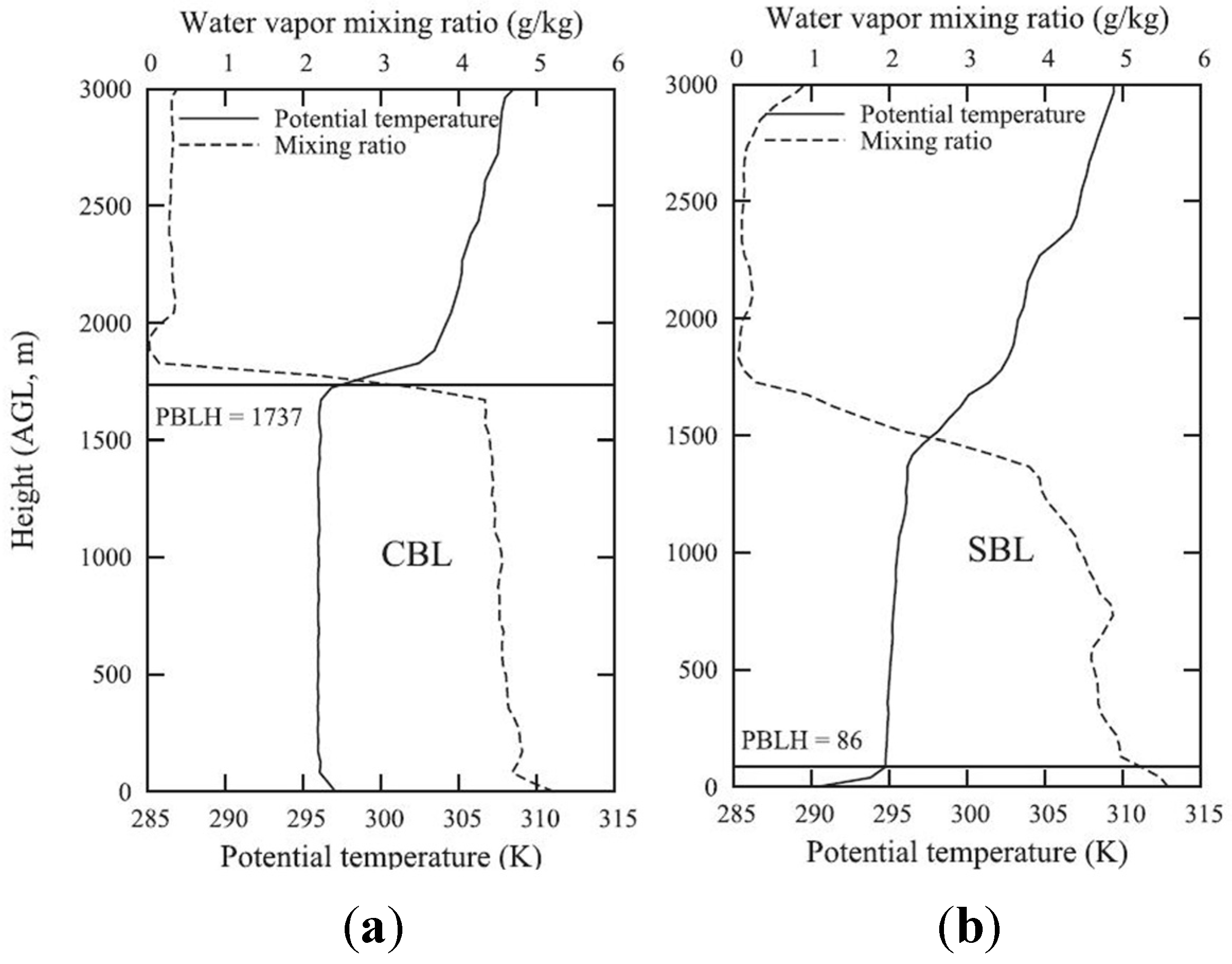
Figure 12.
Case of water vapor mixing ratio and potential temperature profile under convective (
a) and stable air conditions (
b). The horizontal line depicts the position of the determined planetary boundary layer height (PBLH) [
30].
Figure 12.
Case of water vapor mixing ratio and potential temperature profile under convective (
a) and stable air conditions (
b). The horizontal line depicts the position of the determined planetary boundary layer height (PBLH) [
30].
As discussed previously and demonstrated in
Figure 4, for our method, determination of the MH from MODIS profile data under stable conditions can result in substantial error. This appears to be the case for 4 July. The lack of
in situ data under stable air conditions in the Heihe river basin inhibits further verification of our speculation. The radiosonde data from citation [
30], as
Figure 12 showed, indicate the reason for the large difference in the MH from the radiosonde and the MODIS profile data. The MH method applied to radiosonde data in this paper is based on the potential temperature profile; for MODIS data, the MH is derived from the mixing ratio profile; under convective conditions (
Figure 12a), the MH diagnosed from the radiosonde potential temperature profile is consistent with the height of minimum vertical gradient of MR. Consequently, our method for MODIS data based on the MR profile works well under convective conditions; it is different for the stable condition (
Figure 12b), where the MH diagnosed from the radiosonde potential temperature profile is below 100 m, but the height of the abrupt decrease in the MR is about 1500 m, which corresponds to the top of the residual layer of previous days, similar to 4 July,
i.e., 627 m MH for radiosonde and 2156 m for MODIS.
There are caveats associated with using the water vapor profile to diagnose the mixing height: (1) If there is a regular diurnal cycle, especially under stable conditions, the residual layer will also be moist and it is likely that the top of the residual layer is identified instead of the top of the actual ABL; (2) Moist layers in the lower atmosphere do not necessarily indicate local mixing, they could also be advected. Considering the mountainous terrain in the south of the study area, and the fact that it is not as arid as the northern parts of the Heihe river basin, this is a real possibility in the case of southerly winds. This should also receive attention when the method of deriving the MH in the paper applied to other areas, especially where there is a regular diurnal MH cycle or near the coast where moist layers in the lower atmosphere may not indicate the MH, but rather sea-land advection layer during the daytime.
Despite weaknesses, initial estimates of the PBL depth using the atmospheric moisture profile from space-based satellite seem reasonable although more validation is needed. With enough computer resources, this analysis could be extended to provide a global PBL data set using MODIS MOD07 data or relatively high accuracy but low spatial resolution data such as the AIRS product. Our result is also a potential data source for input into global pollutant models. New sources of high accuracy atmospheric moisture profile data with higher vertical resolutions, from future satellites, for example, will promote our method since observation of the atmospheric boundary layer is difficult and expensive using traditional, ground-based methods. If high temporal resolution data from geostationary meteorology satellite show a similar ability as MODIS data for MH calculation, the diurnal variation of MH could also be derived.
6. Conclusion
In this paper, the mixing ratio was selected from primary and conserved variables to identify the MH. The data suggest that the mixing ratio profile can provide evidence of the MH. The MH occurs when there is an abrupt decrease in the mixing ratio (MR). An automated method was developed to obtain the mixing height of the atmospheric boundary layer from MODIS moisture profile data. This study has demonstrated the feasibility of space-based remote sensing of the mixing layer height (MH) without the aid of ground measurements. The methodology for estimating the MH works well on clear-sky days (no clouds) with convective air conditions. However, cloudy skies and stable air conditions may result in large estimation errors. Consequently, cloud and vertical resolution of the atmospheric profile data are two major impediments to the accuracy of our method. Nevertheless, the preliminary results are encouraging both for spatial and temporal variation of the MH. In addition, the MH can be estimated more accurately if higher vertical-resolution data are available.
Acknowledgements
This research was supported by the National Natural Sciences Foundation of China (Number: 41271424 and 91025007), and Special Fund for Grains-scientific Research in the Public Interest (Grant No. 201313009-2). We thank the HiWATER project for providing radiosonde data, and the MODIS data-processing group for atmospheric moisture profile data. We would also like to thank the anonymous reviewers whose useful comments will improve the paper.
Author Contributions
Xueliang Feng was responsible for the implementation of the method used to derive the mixing of the boundary layer, and for data preparation, processing and writing of the manuscript. BingfangWu was responsible for the research design and analysis. Nana Yan provided constructive comments and suggestions.
Conflicts of Interest
The authors declare no conflict of interest.
References
- Stull, R.B. An Introduction to Boundary Layer Meteorology; China Meteorological Press: Beijing, China, 1988; pp. p. 2 and p. 177. (In Chinese) [Google Scholar]
- Garratt, J.R. The Atmospheric Boundary Layer; Cambridge University Press: Cambridge, UK, 1994. [Google Scholar]
- Seibert, P.; Beyrich, F.; Gryning, S.E.; Joffre, S.; Rasmussen, A.; Tercier, P. Review and intercomparison of operational methods for the determination of the mixing height. Atmos. Environ. 2000, 34, 1001–1027. [Google Scholar] [CrossRef]
- Su, Z. The Surface Energy Balance System (SEBS) for estimation of turbulent heat fluxes. Hydrol Earth Syst. Sci. Discuss. 1999, 6, 85–100. [Google Scholar] [CrossRef]
- Kunkel, K.E.; Eloranta, E.W.; Shipley, S.T. Lidar observations of the convective boundary layer. J. Appl. Meteor. 1977, 16, 1306–1311. [Google Scholar] [CrossRef]
- Boers, R.; Eloranta, E.W.; Coulter, R.L. Lidar observations of mixed layer dynamics: Tests of parameterized entrainment models of mixed layer growth rate. J. Clim. Appl. Meteorol. 1984, 23, 247–266. [Google Scholar] [CrossRef]
- Melfi, S.H.; Spinhirne, J.D.; Chou, S.H.; Palm, S.P. Lidar observations of vertically organized convection in the planetary boundary layer over the ocean. J. Clim. Appl. Meteorol. 1985, 24, 806–821. [Google Scholar] [CrossRef]
- Emeis, S.; Münkel, C.; Vogt, S.; Müller, W.J.; Schäfer, K. Atmospheric boundary-layer structure from simultaneous SODAR, RASS and ceilometer measurements. Atmos. Environ. 2004, 38, 273–286. [Google Scholar] [CrossRef]
- Clifford, S.F.; Kaimal, J.C.; Lataitis, R.J.; Strauch, R.G. Ground-based remote profiling in atmospheric studies: An overview. IEEE Proc. 1994, 82, 313–355. [Google Scholar] [CrossRef]
- He, Q.S.; Mao, J.T.; Chen, J.Y.; Hu, Y.Y. Observational and modeling studies of urban atmospheric boundary-layer height and its evolution mechanisms. Atmos. Environ. 2006, 40, 1064–1077. [Google Scholar] [CrossRef]
- Martins, J.; Teixeira, J.; Soares, P.M.M.; Miranda, P.; Kahn, B.H.; Dang, V.T.; Irion, F.W.; Fetzer, E.J.; Fishbein, E. Infrared sounding of the trade-wind boundary layer: AIRS and the RICO experiment. Geophys. Res. Lett. 2010, 37. [Google Scholar] [CrossRef]
- Li, Y.; Zhang, Y.; Liu, J.; Rong, Z.; Zhang, L.; Zhang, Y. Calibration of the visible and near-infrared channels of the FY-2C/FY-2D GEO meteorological satellite at radiometric site. Acta Opt. Sin. 2009, 29, 41–46. [Google Scholar]
- Cheng, G.D. Saving water in the only way for northwest China to survive. Bull. Chin. Acad. Sci. 1996, 10, 203–206. [Google Scholar]
- Cheng, G.D. Integrated Management of the Water-Ecology-Economy System in the Hei River Basin; Science Press: Beijing, Chian, 2009; p. 581. (In Chinese) [Google Scholar]
- Li, X.; Cheng, G.; Liu, S.; Xiao, Q.; Ma, M.; Jin, R.; Che, T.; Xu, Z. Heihe watershed allied telemetry experimental research (HiWATER): Scientific objectives and experimental design. Bull. Am. Meteorol. Soc. 2013, 94, 1145–1160. [Google Scholar] [CrossRef]
- Seemann, S.E.; Borbas, E.E.; Li, J.; Menzel, W.P.; Gumley, L.E. MODIS Atmospheric Profile Retrieval Algorithm Theoretical Basis Document; Cooperative Institute for Meteorological Satellite Studies, University of Wisconsin-Madison: Madison, WI, USA, 2006. [Google Scholar]
- Menut, L.; Flamant, C.; Pelon, J.; Flamant, P.H. Evidence of interaction between synoptic and local scales in the surface layer over the Paris area. Bound.-Lay. Meteorol. 1999, 93, 269–286. [Google Scholar] [CrossRef]
- Granados-Muñoz, M.J.; Navas-Guzmán, F.; Bravo-Aranda, J.A.; Guerrero-Rascado, J.L.; Lyamani, H.; Fernández-Gálvez, J.; Alados-Arboledas, L. Automatic determination of the planetary boundary layer height using Lidar: One-year analysis over southeastern Spain. J. Geophys. Res. 2012, 117, D18. [Google Scholar] [CrossRef]
- Russell, P.B.; Uthe, E.E.; Ludwig, F.L.; Shaw, N.A. A comparison of atmospheric structure as observed with monostatic acoustic sounder and Lidar techniques. J. Geophys. Res. 1974, 79, 5555–5566. [Google Scholar] [CrossRef]
- Martin, C.L.; Fitzjarrald, D.; Garstang, M.; Oliveira, A.P.; Greco, S.; Browell, E. Structure and growth of the mixing layer over the Amazonian rain forest. J. Geophys. Res. 1988, 93, 1361–1375. [Google Scholar] [CrossRef]
- Seidel, D.J.; Ao, C.O.; Li, K. Estimating climatological planetary boundary layer heights from radiosonde observations: Comparison of methods and uncertainty analysis. J. Geophys. Res. 2010, 115. [Google Scholar] [CrossRef]
- McGrath-Spangler, E.L.; Denning, A.S. Estimates of north American summertime planetary boundary layer depths derived from space-borne Lidar. J. Geophys. Res. 2012, 117, D15. [Google Scholar] [CrossRef]
- Wang, G.; Garcia, D.; Liu, Y.; De Jeu, R.; Dolman, A.J. A three-dimensional gap filling method for large geophysical datasets: Application to global satellite soil moisture observations. Environ. Model. Softw. 2012, 30, 139–142. [Google Scholar] [CrossRef]
- Diamantopoulou, M.J. Filling gaps in diameter measurements on standing tree boles in the urban forest of Thessaloniki, Greece. Environ. Model. Softw. 2010, 25, 1857–1865. [Google Scholar] [CrossRef]
- Allen, R.G.; Pereira, L.S.; Raes, D.; Smith, M. Crop evapotranspiration-guidelines for computing crop water requirements-FAO irrigation and drainage paper 56. FAO Rome 1998, 300, D05109. [Google Scholar]
- Jordan, N.S.; Hoff, R.M.; Bacmeister, J.T. Validation of Goddard Earth Observing System-Version 5 MERRA planetary boundary layer heights using CALIPSO. J. Geophys. Res. 2010, 115, D24218. [Google Scholar] [CrossRef]
- Yi, C.; Davis, K.J.; Berger, B.W.; Bakwin, P.S. Long-term observations of the dynamics of the continental planetary boundary layer. J. Atmos. Sci. 2001, 58, 1288–1299. [Google Scholar] [CrossRef]
- Subrahamanyam, D.B.; Anurose, T.J. Solar eclipse induced impacts on sea/land breeze circulation over Thumba: A case study. J. Atmos. Sol.-Terr. Phys. 2011, 73, 703–708. [Google Scholar] [CrossRef]
- Mishra, M.K.; Rajeev, K.; Nair, A.K.M.; Krishna Moorthy, K.; Parameswaran, K. Impact of a noon-time annular solar eclipse on the mixing layer height and vertical distribution of aerosols in the atmospheric boundary layer. J. Atmos. Sol.-Terr. Phys. 2012, 74, 232–237. [Google Scholar] [CrossRef]
- Liu, S.; Liang, X.Z. Observed diurnal cycle climatology of planetary boundary layer height. J. Clim. 2010, 23, 5790–5809. [Google Scholar] [CrossRef]
© 2015 by the authors; licensee MDPI, Basel, Switzerland. This article is an open access article distributed under the terms and conditions of the Creative Commons Attribution license (http://creativecommons.org/licenses/by/4.0/).


