Article

Forecasting Urban Air Quality via a Back-Propagation Neural Network and a Selection Sample Rule

1
School of Engineering, Sun Yat-Sen University, Guangzhou 510275, China
2
Guangdong Provincial Academy of Environmental Science, Guangzhou 510045, China
3
Institute of Advanced Technology, Sun Yat-Sen University, Guangzhou 510275, China
*
Author to whom correspondence should be addressed.
Atmosphere 2015, 6(7), 891-907; https://doi.org/10.3390/atmos6070891
Submission received: 28 April 2015 / Revised: 15 June 2015 / Accepted: 24 June 2015 / Published: 9 July 2015
(This article belongs to the Special Issue Air Quality and Source Apportionment)

Abstract

:
In this paper, based on a sample selection rule and a Back Propagation (BP) neural network, a new model of forecasting daily SO2, NO2, and PM10 concentration in seven sites of Guangzhou was developed using data from January 2006 to April 2012. A meteorological similarity principle was applied in the development of the sample selection rule. The key meteorological factors influencing SO2, NO2, and PM10 daily concentrations as well as weight matrices and threshold matrices were determined. A basic model was then developed based on the improved BP neural network. Improving the basic model, identification of the factor variation consistency was added in the rule, and seven sets of sensitivity experiments in one of the seven sites were conducted to obtain the selected model. A comparison of the basic model from May 2011 to April 2012 in one site showed that the selected model for PM10 displayed better forecasting performance, with Mean Absolute Percentage Error (MAPE) values decreasing by 4% and R2 values increasing from 0.53 to 0.68. Evaluations conducted at the six other sites revealed a similar performance. On the whole, the analysis showed that the models presented here could provide local authorities with reliable and precise predictions and alarms about air quality if used at an operational scale.

1. Introduction

Air quality has recently become a serious issue in several of the large cities in China. This problem has significant potential for adverse impacts on human health and the environment [1,2,3]. Therefore, it is extremely important to accurately forecast the concentrations of pollutants to provide guidance for travel advice and governmental policies.
Forecasting the concentrations of air pollutants represents a difficult task due to the complexity of the physical and chemical processed involved. However, many researchers have been focusing on these types of forecasts [4,5,6,7,8]. The most common forecasting approaches are numerical models and statistical models. Numerical models do not require a large quantity of measured data, but they demand sound knowledge of pollution sources, the chemical composition of the exhaust gases, and the physical processes in the atmospheric boundary layer. This crucial knowledge is often limited. Thus, approximations and simplifications are often employed in the modeling process.
In contrast, statistical models usually necessitate a large quantity of measurement data under a large variety of atmospheric conditions. By applying regression and machine learning techniques, a number of functions can be used to fit the pollution data in terms of selected predictors. Neural networks, a subset of statistical models, are usually presented as systems of interconnected neurons that can compute values from inputs by feeding information through the network. Unlike other statistical models, neural networks make no prior assumptions concerning the data distribution. They can model highly nonlinear functions and can be trained for accurate generalization. These features of the neural network make it an attractive alternative to numerical and other statistical models [9,10,11,12].
There have been many applications of neural networks in air quality forecasting since the 1990s, and researchers have obtained fairly good results [13,14,15,16]. Despite the successful applications of neural networks in the area of atmospheric science, the method has its own weakness and limitations. Studies have shown that there are three main factors that affect neural network effectiveness: network topology, learning algorithm, and learning samples [17,18]. Previous research mainly concentrated on the network structure and learning algorithm, which improved the forecasting accuracy of the network [19,20,21,22,23,24]. However, when improvements in the network structure and learning algorithm reach a certain degree, improvements in the accuracy of the air quality forecasting models plateau. Therefore, the selection of learning samples has become a vital factor that determines the mapping ability and generalization of the network. This is because the selection can ensure the representativeness of the learning samples and remove unnecessary interference, and thereby improve the forecasting accuracy of the model. Harri Niska et al. [21] used a genetic algorithm for selecting the inputs and designing the high-level architecture of a multi-layer perceptron model for forecasting NO2 concentrations. Sousa et al. [22] predicted hourly ozone concentrations based on feed-forward artificial neural networks using principal components as inputs, and they improved the predictions of models by reducing their complexity and eliminating data collinearity.
The main objectives of this paper are to develop a sample filter method for the prediction of the daily NO2, SO2, and PM10 concentration in the Guangzhou Pearl River Delta region based on a similarity principle of weather and pollutant background concentration. During the development of the prediction models, the selection of parameters is conducted by means of sensitivity experiments and the Back Propagation (BP) neural network is used for data-driven computation. The above actions are all part of an integrated environmental strategy designed and run by the local authorities of Guangzhou, according to the demands of the Action Plan on Prevention and Control of Air Pollution. Currently, this action plan is the most rigorous and systematic framework for improving air quality in China.

2. Data

A significant quantity of observational data under a wide variety of atmospheric conditions was required for this study. The dataset in this paper includes meteorological parameters and pollutant concentrations in Guangzhou, which is located in the south central part of Guangdong Province, China (23°06′ N Latitude, 113°15′ E Longitude).
Real-time monitoring meteorological parameters, including temperature, wind speed, wind direction, rainfall, atmospheric pressure, relative humidity, and solar radiation intensity, were obtained from an automatic air quality monitoring station at Sun Yat-Sen University, located in the Haizhu District of Guangzhou City. Forecasting meteorological data, including temperature, wind speed, wind direction, and rainfall, were obtained from Guangzhou Weather Forecasts [25]. All the data were processed into the daily mean value as needed, according to the National Ambient Air Quality Standards (GB 3095-2012) issued by Environment Protection Administration (EPA) of China [26]. The monitoring meteorological data were used as historical meteorological data in the model, and the forecasting meteorological data were used as the meteorological data of the forecasting day. To reduce the interference of different geographic locations on the monitoring meteorological data, pollutant concentration forecasting of seven state-controlled air quality monitoring sites in urban Guangzhou was performed. Thus, the applied monitoring data of the atmospheric environment were derived from the daily pollutant concentration data from seven state-controlled air quality monitoring sites as reported by the Guangzhou Environmental Protection [27]. These state-controlled air quality monitoring sites are the Guangya Middle School (Num. 1), the Guangzhou No. 5 Middle School (Num. 2), the Guangzhou Environmental Monitor Station (Num. 3), the Experimental Kindergarten of Tianhe Vocational School (Num. 4), Luhu Park (Num. 5), Guangdong University of Business Studies (Num. 6), and the Guangzhou No. 86 Middle School (Num. 7). The data span the period from January 2006 to April 2012, and a total of 23,195 valid samples were used for the paper.

3. Methods

In view of the small variation in weather during our study period, a similarity principle of weather and concentration parameters was applied. The multilayer selection rule for historical samples from Guanghzhou was then constructed. This step is very important for the development of predictive models. The selection of historical samples can improve the similarity between the occurrence of historical pollution and future pollution, and a proper selection can improve the efficiency of data-driven models (e.g., BP neural networks). This is also in line with the pollution formation, where the main factor affecting the diffusion and transport of pollutants is the different meteorological parameters, and every meteorological parameter has a different influence on NO2, SO2, and PM10 [28,29]. Thus, the sample selection was based on meteorological similarity and the consistency of the variation trend. The rule was divided into two parts, namely the identification of meteorological parameter similarity and the consistency of the variation trend, i.e., the identification of similarity in background concentrations.
First, a comprehensive correlation analysis of pollutant concentration and meteorological parameters was performed to determine the key factors of the selection rule, and these parameters were also used as inputs into the BP neural network. Next, the three-layer selection sample rule was applied. Finally, we utilized the improved BP neural network for data-driven computation to establish the air quality forecasting model of urban Guangzhou.

3.1. Identification of the Key Factors

A comprehensive correlation analysis of pollutant concentration and meteorological factors was conducted. The number of related days was set to two: the meteorology for the forecasting day and for the day before the forecasting day. Meanwhile, the daily mean value of pollutant concentration two days before the forecasting day was used as an input factor in an attempt to counteract the lack of pollutant emission source data.
A comprehensive analysis of pollutant concentration and meteorological factors was conducted for different pollutants, mainly through correlation analysis and weight analysis of the influencing factors in each pollution scenario. The analysis was intended to identify the degree of influence of each meteorological factor on pollutants, thus resulting in the selection of the factors with the greatest impact on pollutants and the allocation of the corresponding influencing weights. The correlation analysis started with the comparison of two typical pollution scenarios, namely, the ascending or descending periods of each pollutant, and the serious pollution or slight pollution periods. In this way, the degree of influence that the meteorological factors had on pollutants under these two situations was obtained. The average value of the two scenarios was calculated and multiplied with a correlation coefficient to obtain the comprehensive weight of the influence of each meteorological factor on different pollutants.
The ascending and descending periods of each pollutant are defined as the periods when the change in the pollutant concentration between consecutive days exceeds 0.05 mg/m3. Serious pollution or slight pollution are defined as periods when the Air Pollution Index of the pollutant exceeds 100 or is lower than 20, respectively.
The identification of the influencing weight of each meteorological factor under the above-mentioned periods was achieved using the following steps:
(a)
Obtaining the representative data for the meteorological factor
The specific data include the average value of the ascending period M i u , the average value of the descending period M i d , the maximum value of the analysis period M i max , the minimum value M i min of the analysis period, and the overall average value M i adv . The i represents the specific meteorological factor.
(b)
Numerical normalization
(c)
Variation analysis of the meteorological factor ( D i )
D i = M i u M i d M i a d v
(d)
Computation of the influencing weight
w i = D i i = 1 n D i
Finally, the comprehensive influencing weights between meteorology factors and pollutant concentrations were determined by the following equation:
r = R × ( w 1 + w 2 ) / 2
where r is the comprehensive influencing weight between the meteorology factor and the pollutant concentration; R is the correlation coefficient between the meteorology factor and the pollutant concentration; w 1 is the influencing weight in the ascending or descending period; and w 2 is the influencing weight in the serious or slight pollution periods.

3.2. A Selection Sample Rule Based on the Similarity Principle

Multiple meteorological factors create a variety of meteorological parameter spaces that impose different impacts on the transport and diffusion of pollutants. During air quality forecasting, if the appropriate meteorological space is found, the intrinsic relationship between multiple physical quantities and the pollutant will have a reference. An appropriate set of samples was selected for the main influencing factors such that forecasting could be targeted, and the mapping ability and generalization of the network could be improved. Thus, three-layer sample screening principles based on meteorological similarity criteria were proposed.

3.2.1. The Basic Description

The first level of screening identifies samples where the similarity of each meteorological factor reaches a certain threshold value range. The screened samples should conform to the following formula:
Δ y j y j s e t ,   where ,   Δ y j = | y j p r e y j s a m |
where y j p r e is the meteorological factor on the day of forecasting; y j s a m is the meteorological factor of the sample; Δ y j is the meteorological similarity of the meteorology factors between the sample and the day of forecasting; j is the specific meteorological factor; and y j s e t is the threshold value screened by the meteorological factor, forming a primary threshold matrix Y . In this matrix, the threshold value can change dynamically according to the sample size demanded.
The second level of screening applies a threshold value range for total weighted meteorological similarity. The screened samples should conform to the following formula:
S S set ,   where ,   S = j M n u m ( w j Δ y j )
where S is the entire meteorological similarity; Sset is the threshold value screened by the entire meteorological similarity; wj is the weight of each meteorological factor, forming the weight matrix W; and Mnum is the number of meteorological factors.
The third level of screening identifies the n samples with the highest meteorological similarity. The screened samples should conform to the following formula:
Q num n
where Qnum is the number of samples in the sequenced sample column, and n is the number of samples needed.
Among these criteria, the selection of the weight matrices and the threshold matrices is key to obtaining high quality samples. Hence, the following identification approaches for weight matrices and threshold matrices were adopted.

3.2.2. Identification of wj

The establishment of the weight matrix wj was integrated with the selection of model input factors, and a comprehensive correlation analysis of pollutant concentration and meteorological factors was performed. While choosing the input parameters of the neural network, the weight matrix of the selection sample rule was also established.

3.2.3. Identification of y j s e t

The establishment of the threshold matrix y j s e t was accomplished via the orthogonal test method, which is a highly efficient experimental design method used for the arrangement of multi-factor experiments and the search for optimal horizontal combinations [30]. For the different pollutants, we set different levels of factors and selected some representative experimental points (horizontally mixed) for the experiments. The optimal horizontal combination was selected to generate the threshold matrix of the selection sample rule [31].
Based on the results of the above weight matrix w j , the tested experimental factors were identified. In accordance with prior knowledge, the level of each experimental factor was confirmed. The minimum absolute error of the forecasting model was adopted as the experimental objective to seek the optimal combination and finally identify the sample optimization threshold matrix.

3.3. Identification of the Variation Trend Consistency

There will be some scenarios in which wind speed decreases in history but increases on the prediction day compared with the previous day, based on the selection rule stated above in Section 3.2. Such a scenario will lead to an error in the prediction model for use in the BP neural network. Therefore, it is necessary to identify the variation trend consistency.
The factors considered were deduced according to the weight matrix of the selection rule (see Section 3.1) and the principles of the pollution formation. The chosen factors were rainfall, wind speed, and background concentration. However, sensibility experiments were still needed to determine the key factor for NO2, PM10, and SO2. The details of the experimental results will be introduced in the following section.

3.3.1. Variation Trend Consistency for Wind Speed

Because wind speed is a vector, wind speed is described as w x , w y .
w x = w s cos ( w d )   and   w y = w s sin ( w d )
where w s is the recorded wind speed and w d is the recorded wind direction.
Thus, the steps for the identification of the variation trend consistency for wind speed are as follows:
(1)
Calculate the variation between the forecasting day and the day before.
Δ ( w s 1 ) 2 = [ ( w x p ) 2 + ( w y p ) 2 ] [ ( w x p 1 ) 2 + ( w y p 1 ) 2 ]
where Δ ( w s 1 ) 2 is the difference between the squared values of wind speed on the day of forecasting and the day before; w x p and w y p are the two wind vectors on the day of forecasting; and w x p 1 and w y p 1 represent the two wind vectors before the day of forecasting.
(2)
Calculate the variation between the two adjacent days in the samples selected in Section 3.1,
Δ ( w s 2 ) 2 = [ ( w x t ) 2 + ( w y t ) 2 ] [ ( w x t 1 ) 2 + ( w y t 1 ) 2 ]
where Δ ( w s 2 ) 2 is the difference between the squared values of wind speed on the forecasting day and the day before w x t and w y t are the two wind vectors on the forecasting day; and w x t 1 and w y t 1 are the two wind vectors on the day before the forecasting day.
(3)
Identify whether the wind speed in the forecasting data shows the same tendency of ascending or descending as that in the selected samples. If the tendency is the same, the samples are reserved; otherwise, the samples are removed.

3.3.2. The Variation Trend Consistency Identification of Rainfall

The variation in the rainfall levels in the forecasting data was calculated using the following formula:
Δ R F 1 = R F p R F p 1
The variation in the historical rainfall levels was calculated using the following formula:
Δ R F 2 = R F t R F t 1
We then identified whether the rainfall level in the forecasting data showed the same tendency of ascending or descending as that in the sample data. If similar, the samples are reserved; otherwise, the samples are removed.

3.3.3. Similarity Identification of Background Concentration

The following steps were used to conduct the similarity identification of the background concentration:
(1)
The background concentration on the day of forecasting is calculated as follows:
B C 1 = 0.6 B C P - 1 + 0.4 B C P - 2
(2)
The background concentration in the sample data is calculated as follows:
B C 2 = 0.6 B C t- 1 + 0.4 B C t- 2
(3)
Identify whether the background concentration in the forecasting data and the absolute difference of the background concentration on the day of forecasting is in the range of the threshold value. If they are in the range, the samples are reserved; otherwise, they are removed.
A B S ( B C 1 - B C 2 )<= S e t

3.4. Improvements in BP Neural Network

Due to its strong learning and generalization ability, a BP neural network was used as the data-driven computation method [32]. In this paper, a BP neural network with three layers was applied to predict the daily concentrations of NO2, PM10, and SO2. The layers included an input layer, a hidden layer, and an output layer. The data described in Section 2 were divided into training, validation and test sets. The training and validation sets were from January 2006 to April 2011 in seven air quality monitoring sites, of which 80% of these data were randomly selected for the training set; the remaining 20% of the data comprised the validation set. In addition, the data from May 2011 to April 2012 were used for the test set, aiming to test and compare the model performance in seven air quality monitoring sites. There are two main components affecting pollutant concentration: emission sources and pollutant transmission and diffusion conditions. The key factor that affects pollutant transmission and diffusion in a city is the meteorological conditions. Therefore, the meteorological factors identified in Section 3.1 were considered as the major input factors for the BP neural network. According to the conclusions in the literature [33,34], the daily concentrations of NO2, PM10, and SO2 for the two days before the forecasting day were also used as input factors for the BP neural network to reduce the influencefor lacking emissions data. The final number of variables used in the input layer (NInput) in each forecast model is shown in Table 1.
The neuron number of the hidden layer is half that of the input layer [35]. Different neural network structures were established for NO2, PM10, and SO2. The neuron in the output layer was regarded as the forecasted daily concentration of NO2, PM10, and SO2.
The training termination conditions in the BP neural network were also changed to improve the overall accuracy of the forecasting model. When the average relative error of all training samples reached a specified error value, the training would cease. The specified error value was determined by experiments for different error. For NO2, PM10, and SO2, the optimal specified error values were 0.5, 0.4, and 0.35, respectively. Every group training sample was processed five times, which means that five groups of models were developed. The model with the least average relative error was selected as the prediction model, reducing the randomness of the BP neural network.
Table 1. Forecasting results of the seven groups of sensitivity experiments.
PollutantsExperimentsN InputMean
(mg/m3)
MAE
(mg/m3)
MAPERTFAEfAf
SO2Basic (Group 1)100.0270.00937.40.4220500−0.3221.513
RF * (Group 2)100.0270.00936.60.5100.5360.0101.543
WS (Group 3)100.0270.01043.20.3040.464−0.5831.693
BC (Group 4)100.0270.00940.30.3450.483−0.9371.577
RF + WS
(Group 5)
100.0270.00938.50.4300.482−0.1921.501
RF + BC
(Group 6)
100.0270.01149.70.1180.464−1.7261.575
WS + BC
(Group 7)
100.0270.01252.80.1780.393−1.1741.716
PM10basic(Group 1)70.1050.02526.60.5360.4920.2101.297
RF (Group 2)70.1050.02628.80.4760.4330.1081.319
WS (Group 3)70.1050.02526.20.5270.4830.1901.289
BC (Group 4)70.1050.02424.60.5630.5000.2251.280
RF + WS
(Group 5)
70.1050.02527.80.4790.4170.1591.315
RF + BC *
(Group 6)
70.1050.02322.70.6720.5500.3481.269
WS + BC
(Group 7)
70.1050.02426.90.5810.4170.3171.290
NO2Basic (Group 1)100.0730.02025.00.6800.5500.2611.340
RF (Group 2)100.0730.02024.10.6600.5330.1991.345
WS (Group 3)100.0730.01822.70.7020.5330.3521.291
BC (Group 4)100.0730.01923.70.7150.5170.3371.315
RF + WS
(Group 5)
100.0730.01823.70.7230.6170.3861.298
RF + BC
(Group 6)
100.0730.01924.30.7160.4830.3801.306
WS + BC *
(Group 7)
100.0730.01822.50.6880.5670.3971.271
Note: * the Selected Model determined by making experiments.

3.5. Indices of Model Evaluation

We used the following indicators to evaluate the models: Mean absolute error (MAE), Mean Absolute Percentage Error (MAPE), Correlation coefficient (R), tendency forecasting accuracy (TFA), Nash–Sutcliffe coefficient of efficiency (Ef), and Accuracy factor (Af) [36]. The TFA is the forecasting accuracy rate determination for the upward or downward trend of pollutant concentrations over two consecutive days on the basis of monitoring results. Ef, an indicator of the model fit, is a normalized measure (−∞ to 1) that compares the mean square error generated by a particular model simulation to the variance of the target output sequence. An Ef value closer to 1 indicates better model performance; an Ef value of zero indicates that the model is, on average, performing only as good as the use of the mean target value for prediction, and an Ef value < 0 indicates an altogether questionable choice of the model. Af is a simple multiplicative factor indicating the spread of the results around the prediction. The larger the Af value, the less accurate the average estimate.
The MAE, MAPE, TFA, Af and Ef are defined as follows:
M A E = 1 N i = 1 N | y p r e , i y m o n , i |
M A P E = 1 N i = 1 N ( | y p r e , i y m o n , i | y m o n , i × 100 )
T F A = A N
E f = 1 i = 1 N ( y p r e , i y m o n , i ) 2 i = 1 N ( y p r e , i y ¯ m o n ) 2
A f = 10 i = 1 N | log ( y p r e , i y m o n , i ) | N
where y p r e and y m o n are the predicted and measured values, respectively, and y ¯ m o n is the mean of the measured values of the response variable. N is the total number of the observations. A is the number of correct forecasts for the upward or downward trend of pollutant concentrations over two consecutive days.

4. Results and Discussion

4.1. The Results of the Sensitivity Experiments in Guangzhou No. 5 Middle School (Num. 2)

As described in Section 3.3, sensitivity experiments were performed to determine the key factors. The data were obtained from the Guangzhou No. 5 Middle School site. Seven group experiments were performed for SO2, PM10, and NO2. The first experiment (called “Group 1”) was made by the model based on the selection rules described in Section 3.2. That is to say, Group 1 was run using the Basic Model. Besides these selection rules, the second to fourth experiments were conducted based on the variation trend consistency identification of rainfall (RF), wind speed (WS), and background concentration (BC), while the fifth to seventh experiments were considerations of RF + WS, RF + BC, and WS + BC. These experiments were referred to as Group 2, Group 3, Group 4, Group 5, Group 6, and Group 7, respectively. Table 1 summarizes the results of the seven groups of sensitivity experiments. The models with the best performance were selected (termed the Selected Models).
For PM10, the value of Ef and Af of Group 6 were much closer to 1.0 compared with the other models. Compared with Group 1, the Mean Absolute Percentage Error (MAPE) of Group 6 was 4% lower (0.227), R increased by almost 14%, and TFA increased by nearly 6% (0.550). For NO2, Group 7 had the best results with an MAPE of only 0.225, an R value of 0.688, and a TFA value of 0.567. The Ef and Af of Group 7 were 0.397 and 1.271, respectively, which were much closer to 1.0 than the other experiments. Group 2 had the most ideal experimental results for SO2; the MAPE was 0.366, R and TFA were both higher than 0.5, and Ef was the only positive value. In contrast to the PM10 and NO2 results, the SO2 experiments based on BC did not produce the best results. This scenario is perhaps due to a non-obvious variation in daily SO2 concentrations.

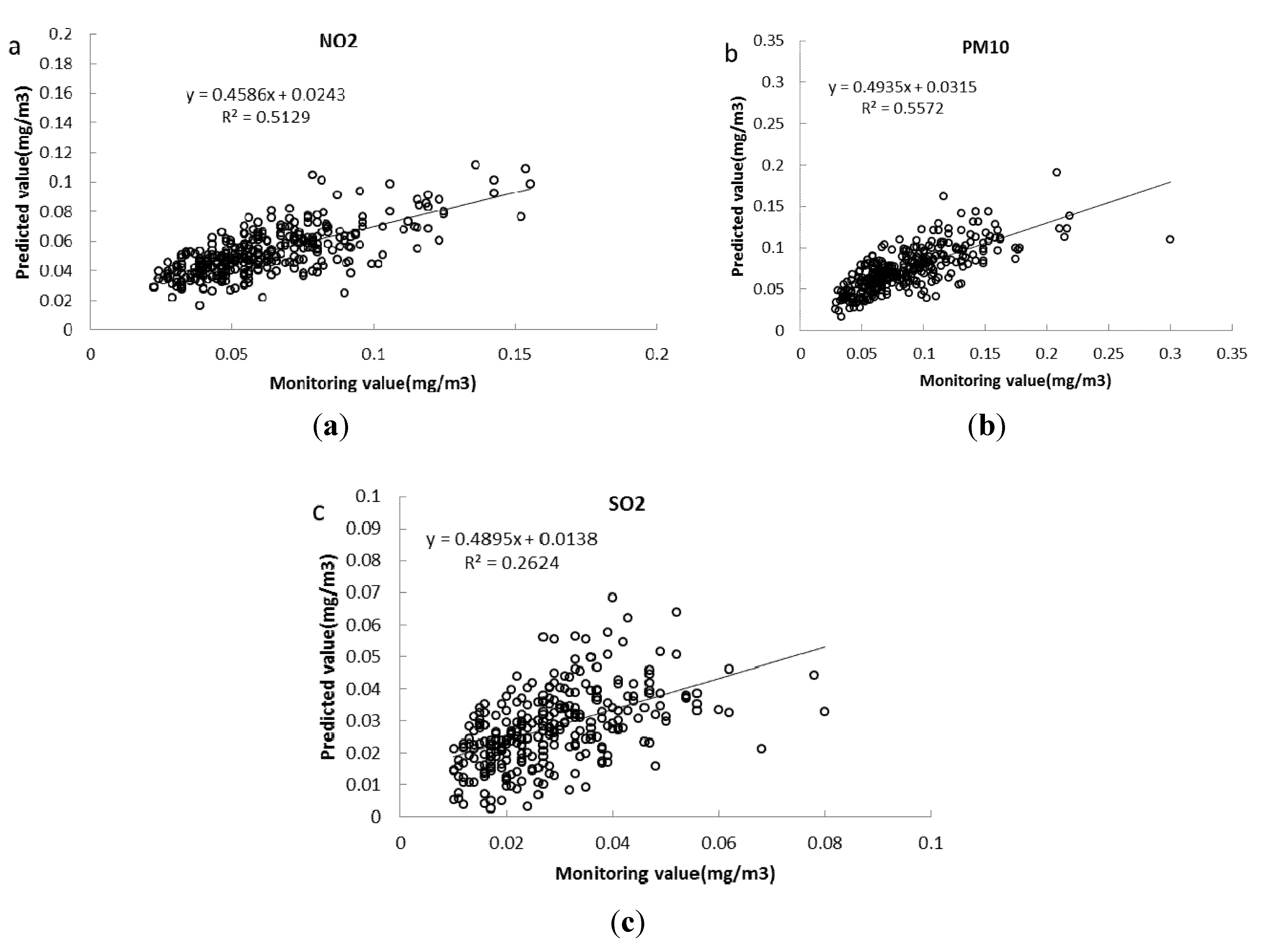
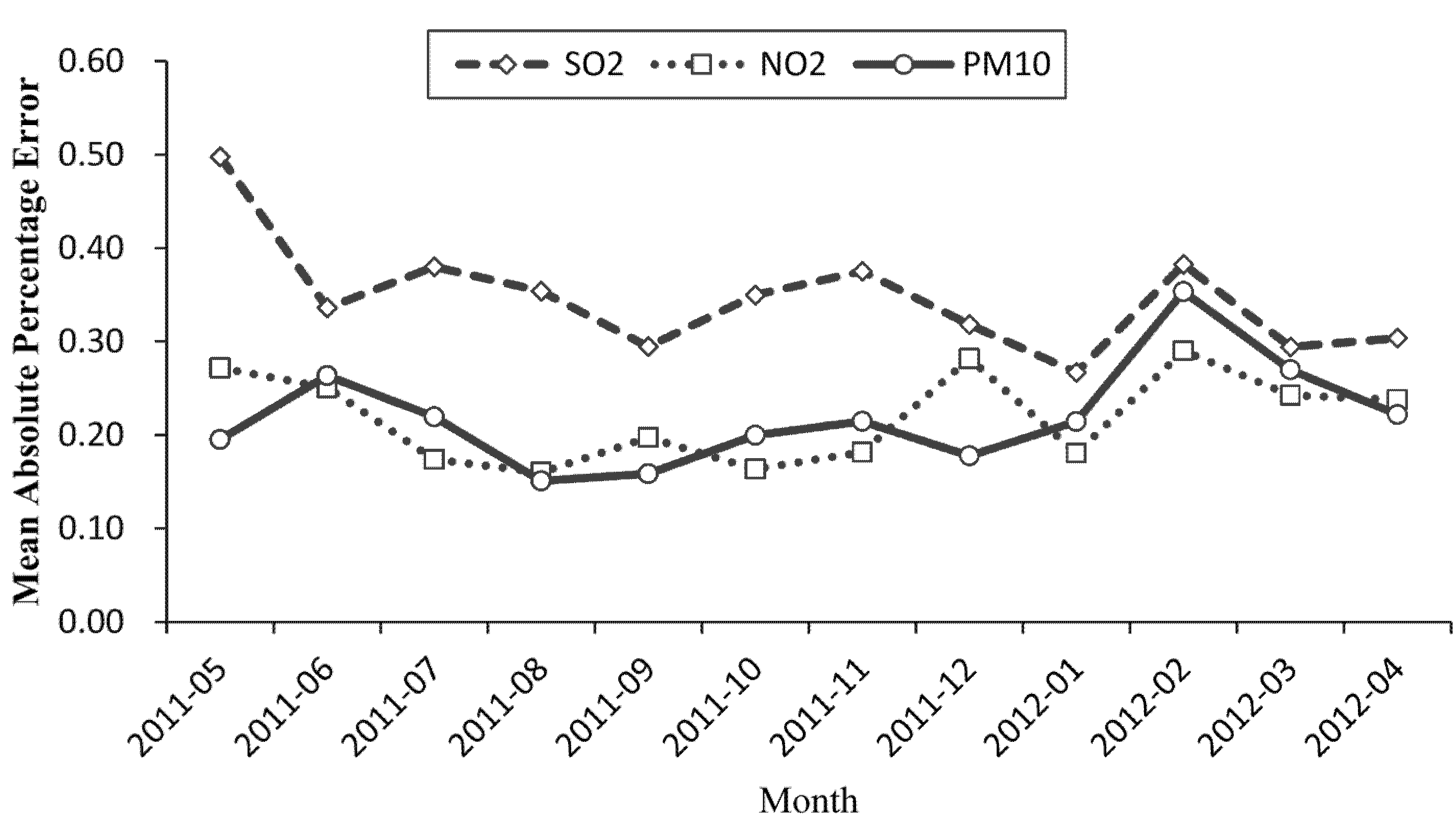
4.2. Errors of the Selected Models of Num. 2 for May 2011 to April 2012

The forecasting results are shown in a scatter diagram of the predicted versus the observed concentrations (Figure 1). The distribution of SO2 is relatively dispersed, which is due to the diversity of the influencing factors and the complexity of dynamic processes. Singh et al. [36] forecast respirable suspended particulate matter (RSPM), SO2, and NO2. The results showed that compared with the two other pollutants, the degree of dispersion in the scatter diagram of the monitored and predicted SO2 values was higher. Kurt et al. [37] used a neural network to build models of SO2, PM10, and CO. The error distribution of the SO2 forecasting model based on the data from two days prior ranged from 37% to 40%, and the model was the least accurate of the three. The distributions of PM10 and NO2 were relatively better, i.e., the line fitted the correlation at 0.5 and above. The forecasting results were stable and the model performed well.
Figure 1. (a-c) Scatter plots of predicted versus observed NO2, PM10, SO2 concentrations for Num. 2.
Atmosphere 06 00891 g001
Errors in the selected model for Guangzhou No. 5 Middle School (Num. 2) from May 2011 to April 2012 are shown in Figure 2. Overall, the monthly prediction accuracy of SO2 was higher than PM10 and NO2, and the NO2 model performed better than the PM10 model. The highest errors for SO2, PM10, and NO2 were observed in February, where the daily concentrations were almost the highest due to the bad weather; the BP neural network is not sensitive to extremely high or low values [33,34]. However, the MAPE of the SO2, PM10, and NO2 models were 0.383, 0.353, and 0.290, respectively. These MAPE values are acceptable for operational forecasts.
Figure 2. MAPE of models for Num. 2 from May 2011 to April 2012.
Atmosphere 06 00891 g002

4.3. Errors in the Selected Models for Others Sites

The selected model for SO2, NO2, and PM10 was tested in the remaining six sites (detailed description in Section 2) in the urban district of Guangzhou, and a comparison was made between the Selected Model and the Basic Model. The results are shown in Table 2. On the whole, the Selected Model was equal to or better than the Basic Model for SO2, NO2, and PM10. As for SO2, the MAPE of the Selected Model decreased from 0.417 to 0.377, the correlation increased from 0.409 to 0.477, the TFA increased from 0.490 to 0.517. In addition, the Ef and Af were closer to 1 compared with the Basic Model. Adding the sample optimization rules to the variation tendency identification of the rainfall level changes improved the forecast accuracy of the different pollutants to different degrees at every site. For PM10, the MAPE of the Selected Model was 0.250 for the six sites, which was almost 0.10 lower than that of the Basic model. The correlation was greater than 0.7, and the TFA increased by 24%, from 0.421 to 0.523. Adding the variation tendency identification of the rainfall level changes and the similarity identification of the background concentrations to the model resulted in an effective improvement of the forecast accuracy of PM10. Regarding NO2, adding the variation tendency identification of the wind speed changes and the similarity identification of the background concentrations did not greatly improve the forecast results. The Selected Model is useful for the six sites, and the errors of the model are acceptable for application purposes.
Table 2. Comparisons between the Selected and Basic Model in the remaining six sites.
PollutantSiteModelMean (mg/m3)MAE (mg/m3)MAPERTFAEfAf
SO2Num. 1Basic0.0240.00836.80.5250.5060.1591.459
Selected0.0240.00834.90.6140.5250.2371.451
Num. 3Basic0.0270.01043.60.4180.511−0.1641.539
Selected0.0270.01040.40.4090.475−0.1811.548
Num. 4Basic0.0230.00944.20.3940.509−0.3011.567
Selected0.0230.00941.30.4560.527−0.3321.541
Num. 5basic0.0220.00735.60.4410.455−0.0191.468
Selected0.0220.00731.60.4720.5150.0591.408
Num. 6Basic0.0270.01142.80.3550.4660.0551.587
Selected0.0270.01039.60.4510.5080.0191.551
Num. 7basic0.0360.01547.80.2980.527−0.5801.662
Selected0.0360.01341.20.4220.561−0.2391.563
PM10Num. 1Basic0.0830.02326.20.6560.4380.3481.328
Selected0.0830.02224.90.7130.5090.3971.335
Num. 3Basic0.0670.01832.10.6040.1320.3481.354
Selected0.0670.01826.80.6940.5420.4591.322
Num. 4basic0.0610.01731.60.6800.4930.4541.350
Selected0.0610.01726.40.7410.5060.5231.317
Num. 5basic0.0670.01624.70.7420.4650.5371.268
Selected0.0670.01622.70.7290.5310.4871.267
Num. 6Basic0.0630.01830.40.5830.4930.3011.358
Selected0.0630.01929.20.5890.4920.2471.390
Num. 7basic0.0870.02225.40.6820.4670.4081.308
Selected0.0870.02223.30.7170.5250.4311.288
NO2Num. 1basic0.0610.01320.90.6880.4830.3921.248
Selected0.0610.01320.50.7150.5000.4481.243
Num. 3Basic0.0680.01622.20.5960.4630.2261.272
Selected0.0680.01521.50.6760.5570.3201.266
Num. 4Basic0.0520.01021.90.6850.5110.4561.232
Selected0.0520.01019.30.7220.5410.5021.215
Num. 5Basic0.0380.00925.80.6130.4540.3631.285
Selected0.0380.00923.00.5990.4620.3081.267
Num. 6Basic0.0530.01426.80.7570.4970.4051.337
Selected0.0530.01524.60.7280.5280.3101.334
Num. 7Basic0.0410.01027.40.6680.4760.4351.305
Selected0.0410.00923.10.7000.5050.4651.269

5. Conclusions

In this paper, based on a selection sample rule and BP neural network, a new model of forecasting daily SO2, NO2, and PM10 concentrations in seven Guangzhou sites was developed.
(1)
A meteorological similarity principle was applied in the development of the selection sample rule. Key meteorological factors influencing the daily SO2, NO2, and PM10 concentrations were determined and weight matrices and threshold matrices were generated. A basic model was then developed based on the improved BP neural network. The selection sample rule consisted of three layers.
(2)
In improving the basic model, identification of the variation consistency of some factors was added in the rule, and seven sets of sensitivity experiments (one in each of the seven sites) were conducted to obtain the selected model. These experiments determined that the variation consistency of the rainfall level added to the SO2 forecast model, the rainfall level variation tendency and the background concentration similarity identification added to the PM10 forecast model, while wind speed variation identification and background concentration similarity identification added to the NO2 forecast model. The improved BP neural network was also used for data-driven computation.
(3)
Evaluations in the site by comparison of the basic model from May 2011 to April 2012 showed the selected model for PM10 displayed better forecasting performance, with MAPE values decreasing by 4% and R2 values increasing from 0.53 to 0.68. The selected model for NO2 had little improvements compared with the basic model, while the MAPE values of the selected model for SO2 were as high as 36.6% with R2 values of 0.51.
(4)
Evaluations conducted at the six other sites revealed similar performances. The MAPE values of the selected models for SO2, PM10, and NO2 were 37.7%, 25.0%, and 22.0%, respectively. Of course, the above results showed that the SO2 model may be further improved in future research, by developing a combined model or by considering the interaction of atmospheric pollutants.

Acknowledgments

This work was completely supported by the National Natural Science Foundation of China (No. 51108471).

Author Contributions

Yonghong Liu, Qianru Zhu conceived and designed the model and experiments; Dawen Yao and Weijia Xu collected and analyzed the data; Yonghong Liu wrote the paper.

Conflicts of Interest

The authors declare no conflict of interest.

References

  1. Dimitriou, K.; Kassomenos, P.A.; Paschalidou, A.K. Assessing air quality with regards to its effect on human health in the European Union through air quality indices. Ecol. Indic. 2013, 27, 108–115. [Google Scholar] [CrossRef]
  2. Pope, C.A., III; Burnett, R.T.; Thun, M.J.; Calle, E.E.; Krewski, D.; Ito, K.; Thurston, G.D. Lung cancer, cardiopulmonary mortality, and long-term exposure to fine particulate air pollution. JAMA 2002, 287, 1132–1141. [Google Scholar] [CrossRef] [PubMed]
  3. Li, G.; Sang, N. Delayed rectifier potassium channels are involved in SO2 derivative-induced hippocampal neuronal injury. Ecotoxicol. Environ. Saf. 2009, 72, 236–241. [Google Scholar] [CrossRef] [PubMed]
  4. Juhos, I.; Makra, L.; Tóth, B. Forecasting of traffic origin NO and NO2 concentrations by Support Vector Machines and neural networks using Principal Component Analysis. Simul. Model. Pract. Theory 2008, 16, 1488–1502. [Google Scholar] [CrossRef]
  5. Finardi, S.; de Maria, R.; D’Allura, A.; Cascone, C.; Calori, G.; Lollobrigida, F. A deterministic air quality forecasting system for Torino urban area, Italy. Environ. Model. Softw. 2008, 23, 344–355. [Google Scholar] [CrossRef]
  6. Dong, M.; Yang, D.; Kuang, Y.; He, D.; Erdal, S.; Kenski, D. PM2.5 concentration prediction using hidden semi-Markov model-based times series data mining. Expert Syst. Appl. 2009, 36, 9046–9055. [Google Scholar] [CrossRef]
  7. Pai, T.Y.; Ho, C.L.; Chen, S.W.; Lo, H.M.; Sung, P.J.; Lin, S.W.; Lai, W.J.; Tseng, S.C.; Ciou, S.P.; Kuo, J.L.; Kao, J.T. Using seven types of GM (1, 1) model to forecast hourly particulate matter concentration in Banciao City of Taiwan. Water Air Soil Pollut. 2011, 217, 25–33. [Google Scholar] [CrossRef]
  8. Pai, T.Y.; Hanaki, K.; Chiou, R.J. Forecasting Hourly Roadside Particulate Matter in Taipei County of Taiwan Based on First-Order and One-Variable Grey Model. CLEAN Soil Air Water 2013, 41, 737–742. [Google Scholar] [CrossRef]
  9. Comrie, A.C. Comparing neural networks and regression models for ozone forecasting. J. Air Waste Manag. Assoc. 1997, 47, 653–663. [Google Scholar] [CrossRef]
  10. Schlink, U.; Dorling, S.; Pelikan, E.; Nunnari, G.; Cawley, G.; Junnine, H.; Greig, A.; Foxall, R.; Eben, K.; Chatterton, T.; et al. A rigorous inter-comparison of ground-level ozone predictions. Atmos. Environ. 2003, 37, 3237–3253. [Google Scholar] [CrossRef]
  11. Kukkonen, J.; Partanen, L.; Karppinen, A.; Ruuskanen, J.; Junninen, H.; Kolehmainen, M.; Niska, H.; Dorling, S.; Chatterton, T.; Foxall, R.; et al. Extensive evaluation of neural network models for the prediction of NO2 and PM10 concentrations, compared with a deterministic modelling system and measurements in central Helsinki. Atmos. Environ. 2003, 37, 4539–4550. [Google Scholar] [CrossRef]
  12. Diaz-Robles, L.A.; Ortega, J.C.; Fu, J.S.; Reed, G.D.; Chow, J.C.; Watson, J.G.; Moncada-Herrera, J.A. A hybrid ARIMA and artificial neural networks model to forecast particulate matter in urban areas: The case of Temuco, Chile. Atmos. Environ. 2008, 42, 8331–8340. [Google Scholar] [CrossRef]
  13. Yi, J.; Prybutok, V.R. A neural network model forecasting for prediction of daily maximum ozone concentration in an industrialized urban area. Environ. Pollut. 1996, 92, 349–357. [Google Scholar] [CrossRef]
  14. Grivas, G.; Chaloulakou, A. Artificial neural network models for prediction of PM10 hourly concentrations, in the Greater Area of Athens, Greece. Atmos. Environ. 2006, 40, 1216–1229. [Google Scholar] [CrossRef]
  15. Hooyberghs, J.; Mensink, C.; Dumont, G.; Fierens, F.; Brasseur, O. A neural network forecast for daily average PM10 concentrations in Belgium. Atmos. Environ. 2005, 39, 3279–3289. [Google Scholar] [CrossRef]
  16. Paschalidou, A.K.; Karakitsios, S.; Kleanthous, S.; Kassomenos, P.A. Forecasting hourly PM10 concentration in Cyprus through artificial neural networks and multiple regression models: Implications to local environmental management. Environ. Sci. Pollut. Res. 2011, 18, 316–327. [Google Scholar] [CrossRef] [PubMed]
  17. Zhang, G.; Eddy Patuwo, B.; Hu, Y.M. Forecasting with artificial neural networks: The state of the art. Int. J. Forecast. 1998, 14, 35–62. [Google Scholar] [CrossRef]
  18. Gardner, M.W.; Dorling, S.R. Artificial neural networks (the multilayer perceptron)—A review of applications in the atmospheric sciences. Atmos. Environ. 1998, 32, 2627–2636. [Google Scholar] [CrossRef]
  19. Kolehmainen, M.; Martikainen, H.; Ruuskanen, J. Neural networks and periodic components used in air quality forecasting. Atmos. Environ. 2001, 35, 815–825. [Google Scholar] [CrossRef]
  20. Lu, W.Z.; Fan, H.Y.; Lo, S.M. Application of evolutionary neural network method in predicting pollutant levels in downtown area of Hong Kong. Neurocomputing 2003, 51, 387–400. [Google Scholar] [CrossRef]
  21. Niska, H.; Hiltunen, T.; Karppinen, A.; Ruuskanen, J.; Kolehmainen, M. Evolving the neural network model for forecasting air pollution time series. Eng. Appl. Artif. Intell. 2004, 17, 159–167. [Google Scholar] [CrossRef]
  22. Sousa, S.I.V.; Martins, F.G.; Alvim-Ferraz, M.C.M.; Pereira, M.C. Multiple linear regression and artificial neural networks based on principal components to predict ozone concentrations. Environ. Model. Softw. 2007, 22, 97–103. [Google Scholar] [CrossRef]
  23. Al-Alawi, S.M.; Abdul-Wahab, S.A.; Bakheit, C.S. Combining principal component regression and artificial neural networks for more accurate predictions of ground-level ozone. Environ. Model. Softw. 2008, 23, 396–403. [Google Scholar] [CrossRef]
  24. Pires, J.C.M.; Gonçalves, B.; Azevedo, F.G.; Carneiro, A.P.; Rego, N.; Assembleia, A.J.B.; Silva, P.A.; Lima, J.F.B.; Alves, C.; Martins, F.G. Optimization of artificial neural network models through genetic algorithms for surface ozone concentration forecasting. Environ. Sci. Pollut. Res. 2012, 19, 3228–3234. [Google Scholar] [CrossRef] [PubMed]
  25. Guangzhou Weather Forecasts. Available online: http://www.tqyb.com.cn/ (accessed on 1 January 2013).
  26. Ministry of Environmental Protection of China. Ambient Air Quality Standards; China Environmental Science Press: Beijing, China, 2012.
  27. Guangzhou Environmental Protection. Available online: http://www.gzepb.gov.cn/comm/apidate.asp (accessed on 1 January 2013).
  28. Elminir, H.K. Dependence of urban air pollutants on meteorology. Sci. Total Environ. 2005, 350, 225–237. [Google Scholar] [CrossRef] [PubMed]
  29. Pearce, J.L.; Beringer, J.; Nicholls, N.; Hyndman, R.J.; Tapper, N.J. Quantifying the influence of local meteorology on air quality using generalized additive models. Atmos. Environ. 2011, 45, 1328–1336. [Google Scholar] [CrossRef]
  30. Yu, Z.Y.; Yuan, J.Y.; Yu, Y.; Zhang, W.; Wu, Z.H. Research on Relationship of Control Parameters of Cement Concrete Strength by Orthogonal Test Method. J. Huangshi Inst. Technol. 2012, 3, 38–41. [Google Scholar]
  31. Lin, Y.; Yang, X.G.; MA, Y.Y. An Analysis of Factors Causing Congestion with the Application of Orthogonal Experimental Design Method. Syst. Eng. 2005, 10, 39–43. [Google Scholar]
  32. Hornik, K.; Stinchcombe, M.; White, H. Multilayer feedforward networks are universal approximators. Neural Netw. 1989, 2, 359–366. [Google Scholar] [CrossRef]
  33. Li, L. Study on urban air quality forecast model based on adaptive artificial neural network. M.Sc. Thesis, Sun Yet-Sen University, Guangzhou, China, 2011. [Google Scholar]
  34. Zhu, Q.R. Study on combined urban air quality forecast model. M.Sc. Thesis, Sun Yet-sen University, Guangzhou, China, 2013. [Google Scholar]
  35. Cai, M.; Yin, Y.; Xie, M. Prediction of hourly air pollutant concentrations near urban arterials using artificial neural network approach. Transp. Res. Part D Transp. Environ. 2009, 14, 32–41. [Google Scholar] [CrossRef]
  36. Singh, K.P.; Gupta, S.; Kumar, A.; Shukla, S.P. Linear and nonlinear modeling approaches for urban air quality prediction. Sci. Total Environ. 2012, 426, 244–255. [Google Scholar] [CrossRef] [PubMed]
  37. Kurt, A.; Oktay, A.B. Forecasting air pollutant indicator levels with geographic models 3days in advance using neural networks. Expert Syst. Appl. 2010, 37, 7986–7992. [Google Scholar] [CrossRef]

