Impact of Coupled NO_x/Aerosol Aircraft Emissions on Ozone Photochemistry and Radiative Forcing

Abstract

Three global chemistry-transport models (CTM) are used to quantify the radiative forcing (RF) from aviation NO_x emissions, and the resultant reductions in RF from coupling NO_x to aerosols via heterogeneous chemistry. One of the models calculates the changes due to aviation black carbon (BC) and sulphate aerosols and their direct RF, as well as the BC indirect effect on cirrus cloudiness. The surface area density of sulphate aerosols is then passed to the other models to compare the resulting photochemical perturbations on NO_x through heterogeneous chemical reactions. The perturbation on O₃ and CH₄ (via OH) is finally evaluated, considering both short- and long-term O₃ responses. Ozone RF is calculated using the monthly averaged output of the three CTMs in two independent radiative transfer codes. According to the models, column ozone and CH₄ lifetime changes due to coupled NO_x/aerosol emissions are, on average, +0.56 Dobson Units (DU) and −1.1 months, respectively, for atmospheric conditions and aviation emissions representative of the year 2006, with an RF of +16.4 and −10.2 mW/m² for O₃ and CH₄, respectively. Sulphate aerosol induced changes on ozone column and CH₄ lifetime account for −0.028 DU and +0.04 months, respectively, with corresponding RFs of −0.63 and +0.36 mW/m². Soot-cirrus forcing is calculated to be 4.9 mW/m².

1. Introduction

Aviation alters the composition of the atmosphere globally and can thus drive climate and ozone changes [1,2]. Aircraft emissions may impact the atmospheric composition both directly (mainly via emissions of CO₂, H₂O, NO_x, SO₂, soot) and indirectly (by increasing tropospheric O₃ and OH and decreasing the CH₄ lifetime; with formation of contrails and with indirect effects on upper tropospheric cirrus cloudiness, i.e., contrail-cirrus and soot-cirrus). The majority of the emitted species produced by combustion of kerosene are gases and soot particles. The former may be directly relevant as greenhouse gases (CO₂ and stratospheric H₂O), while the latter may trigger cloud formation. In addition, the combustion process forms numerous trace species, such as NO, NO₂, SO₂, CO and hydrocarbons (HCs). NO_x emissions, in particular, play a key role in tropospheric and lower stratospheric chemistry, by enhancing the ozone production and the OH concentration [3,4]. The chemical reaction with OH, in turn, acts as the main sink for atmospheric CH₄, so that NO_x emission by the aircraft will decrease its lifetime. The lowering of CH₄ atmospheric abundance induces a cooling that may partially counteract the warming due to the other greenhouse gases (CO₂, stratospheric H₂O, tropospheric O₃), as well as the warming due to upper tropospheric particle formation (contrails and aviation cirrus cloudiness) [5]. In addition, the aircraft impact on atmosphere and climate may act on very different time scales, inducing long-term responses with CO₂ accumulation and CH₄ lifetime changes or producing short-term climate responses with additional O₃ production and by increasing aerosols and cloud particles. The aircraft impact on atmospheric ozone is particularly complex, because a superposition of short- and long-term effects takes place, via direct NO_x emissions (short-term) and via OH driven CH₄ changes that can feedback, in turn, on HO_x chemistry and finally on ozone (long-term) [5]. The dilution of aircraft plumes increases the complexity of this problem. Kraabøl et al. [6] found ~20% reduction in O₃-changes caused by aircraft NO_x; Cariolle et al. [7] found the reduction to be in the range of 10%–25%. However, a possible impact on CH₄ is uncertain.

Most of the aircraft emitted SO₂is localized in the upper troposphere where is oxidized via OH radicals producing SO₃, which via reaction with water vapour, is rapidly converted to gaseous H₂SO₄; where gaseous H₂SO₄ represents an important aerosol precursor, and through heterogeneous reactions has an impact on ozone chemistry [8,9,10]. Among the emitted gases and gaseous products formed in the very young plume are condensable gases. These may undergo condensation in the young plume leading to volatile aerosol particles and volatile coating of soot. Small soot particles may combine with larger particles, and when large enough, they may act as condensation nuclei, which potentially play an important role in changing the occurrence of natural cirrus and its properties [11]. The aviation impact on upper tropospheric cirrus cloudiness may take place as line-shaped contrails that persist and spread into cirrus-like clouds. (i.e., contrail-cirrus) or with heterogeneous freezing of adiabatically ascending water vapour on soot aerosol particles (i.e., soot-cirrus, formed in the absence of spreading contrails). Aircraft soot emissions can possibly affect natural cloudiness by slightly reducing water vapour available for the formation of natural clouds. Burkhardt and Kärcher [12] have found that the change in the water budget due to contrail-cirrus formation could reduce natural cirrus by about 1%–2% in some regions at the main cruise altitudes.

The most important particles produced by aircraft emissions that affect atmospheric chemistry are those of sulphuric acid (H₂SO₄). They act through heterogeneous chemical reactions where NO_xconversion into nitric acid may take place on the surface of these aerosols: This reduces O₃ production via NO_x reactions with HO₂ and organic radicals RO₂. Because of the very small size of aircraft-generated particles and since emissions occur mostly at mid-latitudes (in the Northern Hemisphere), the relevant heterogeneous reactions are essentially hydrolysis of N₂O₅ and BrONO₂ [13]; their rates are treated following JPL recommendations [14]. The main effect of these two reactions is twofold: (a) NO_x enhancements from NO_x aircraft emissions are partly counter-balanced by additional heterogeneous conversion of NO_x into HNO₃ on these particles in the flight corridors, with decreased O₃ production caused by peroxy radicals and sunlight; (b) this reduced NO_x enhancement tends to increase the amount of reactive Cl and Br in the high latitude lowermost stratosphere, since less Cl/Br can be stored into Cl and Br nitrates, which enhances O₃ depletion via catalytic Cl and Br cycles.

Aircraft emissions may perturb the global amount and the size distribution of H₂SO₄ aerosols in two ways: (a) the direct emission of ultrafine particles (radius~5 nm) [15,16,17] and (b) the release of gas phase SO₂ [8]. Direct particle emissions are estimated to be 4%–15% of the overall aircraft emitted sulphur [16,18]. These direct particle emissions do not significantly change aerosol mass and extinction but they may substantially increase the sulphate aerosol surface area density (SAD) in the Northern Hemisphere upper troposphere and lower stratosphere (UTLS). Release of gas phase SO₂, on the other hand, may increase the net production of H₂SO₄, thus enhancing the sulphate mass in the accumulation mode and consequently, the direct radiative forcing (RF). It also may increase the gas phase contribution to SAD, in the range of 25% of the change produced by direct plume particle emission [8,9].

In this work, we focus on the impact of aircraft emitted NO_x on tropospheric and lower stratospheric O₃ formation and loss, also taking into account the effects that emitted sulphur has on UTLS NO_x, via heterogeneous reactions on sulphate aerosol SAD. The tropopause radiative forcing associated with ozone changes is also evaluated using monthly averaged three-dimensional output from three independent global models (ULAQ-CTM, Oslo CTM2, Oslo CTM3), feeding two well-tested and documented off-line radiative transfer models (ULAQ, Oslo). The RF due to sulphate and black carbon (BC) soot particles is evaluated in the ULAQ-CTM, taking into account both the direct forcing due to radiation scattering/absorption and also the indirect effects due to formation of soot-cirrus ice particles. First, we use the University of L’Aquila model ULAQ-CTM, with fully coupled aerosols and chemistry, to assess this impact. Then, the Oslo models CTM3 and CTM2 were also applied to robustly test the chemical impact of aerosols. As these models do not include the required coupled aerosol-chemistry, their heterogeneous reactions were described by monthly averages of aerosol SAD from the ULAQ-CTM. These models are briefly described in this paper, as well as the ULAQ-CTM results in terms of background atmospheric aerosols and their perturbations due to aviation emissions. Finally, a detailed discussion of the radiative calculations on the NO_x/aerosol coupled impact on ozone is presented.

The multi-model evaluation of the short-term ozone RF along with the estimated BC indirect effect on cirrus cloudiness (soot-cirrus) are two important advances in the present study with respect to Pitari et al. [9]. Soot-cirrus is integrated in the representation of ice clouds in the ULAQ-CTM, discriminating between natural cirrus cloudiness formed through homogeneous freezing of adiabatically ascending water vapour [19] and ice particles formed via heterogeneous freezing on non-hydrophobic BC particles [11]. Gettelman and Chen [20] have documented modeling results on direct and indirect effects of aviation aerosols on climate (BC, SO₄ and induced cloudiness). Another new insight from the present study is the evaluation of the long-term O₃ negative RF associated with CH₄ lifetime changes produced by the aviation induced tropospheric OH perturbation. In this case, we have followed an innovative approach, using not only IPCC-type parametric formulas to calculate long-term negative RFs associated with the CH₄ RF (i.e., tropospheric O₃ and stratospheric H₂O), but designed an experiment (ULAQ_FLX) where surface CH₄ is calculated using a flux boundary conditions. In this way, the calculated OH change due to aircraft NO_x emissions produces a CH₄ lifetime change that may directly migrate onto the CH₄ mixing ratio distribution. Therefore, the calculated O₃ RF results to be the sum of both the short- and long-term responses and the effects on stratospheric H₂O are explicitly calculated. Another recently published modeling work that has focused on NO_x/aerosol interaction is Unger [21]. The general effects of aviation NO_x have been widely discussed in the modeling community, e.g., by Köhler et al. [3], Hoor et al. [4], Grewe et al. [22], Holmes et al. [5], Gottschaldt et al. [23], with insights in many relevant aspects of the problem (photochemistry, sensitivity approach, climate, uncertainties).

2. Experimental Section

A short description of the chemistry-transport models used in this study and their basic setups are presented in the following subsections, along with a description of the adopted aviation emission inventories and an overall presentation of the numerical experiment setup. Details on the model adopted surface emissions of NO_x, CO and VOC are reported in Søvde et al. [24].

2.1. ULAQ-CTM

The University of L’Aquila model is a global scale climate-chemistry coupled model (ULAQ-CCM) extending from the surface to the mesosphere (0.04 hPa). In this study, the ULAQ-CCM was operated in CTM mode. Dynamical data, i.e., velocity stream-function and velocity potential, are provided by the background GCM run in a reference case, with no feedbacks of aviation-induced changes. The ULAQ-CCM has been fully described in Pitari et al. [25] and also in Eyring et al. [26] and Morgenstern et al. [27] for the SPARC (i.e., Stratospheric Processes And their Role in Climate) climate-chemistry model validation (CCMVal) campaign. The most recent version of the ULAQ model has been fully documented in Pitari et al. [28], with some important updates with respect to the SPARC-CCMVal exercise. These are: (a) increase of horizontal and vertical resolution, now T21 with 126 log-pressure levels (with approximate pressure altitude increment of 568 m); (b) inclusion of a parameterization for the formation of upper tropospheric cirrus cloud ice particles [19]; (c) update to Sander et al. [14] recommendations for reaction rates of homogeneous and heterogeneous chemistry, cross sections of species, and the parameterization of Minschwaner et al. [29] for the Schumann-Runge bands, based on fixed-temperature opacity distribution function formulation; (d) new radiative transfer code for calculations of photolysis, solar heating rates and top-of-atmosphere radiative forcing. The oceanic surface temperature is assimilated from the Hadley Centre for Climatic Prediction and Research [30]. A parameterization of periodic natural forcings (solar cycle, quasi-biennial oscillation) is included on-line.

The chemistry module is organized by long-lived and surface-flux species (CH₄, N₂O, CFCs, HCFCs, CO, NO_x, NMVOC (i.e., non-methane volatile organic compounds)) and by all medium and short-lived species grouped in the families O_x, NO_y, HO_x, CHO_x, Cl_y, Br_y, SO_x, and aerosols. In total, there are 40 transported species, 26 species at photochemical equilibrium, and 57 size categories for the aerosols. The photochemistry module is organized with 140 gas-phase reactions, 45 photolysis reactions and 30 heterogeneous reactions on the surface of sulphate aerosols, nitric acid trihydrate and ice particles [25,31] or water droplets. All reaction and photolysis rates are treated according to JPL recommendations [14]. In the specific case of N₂O₅ hydrolysis on sulphate aerosols, the ULAQ model includes an explicit dependence from aerosol acidity (which in turn depends on temperature and pressure); gaseous HNO₃ is released from this reaction, both in the stratosphere and troposphere. An evaluation example of the ULAQ model tropospheric chemistry is given in Brunner et al. [32]. The model includes the major components of stratospheric and tropospheric aerosols (sulphate, carbonaceous, soil dust, sea salt, PSCs). Nitrate aerosols (i.e., ammonium nitrate) are not explicitly considered in the ULAQ aerosol module. This is not expected to be a significant sink term for HNO₃ from aircraft NO_x, since NH₃ originates from ground sources, is highly reactive and easily removed by wet and dry deposition and not present in significant concentrations at cruise altitudes. The updated radiative transfer module operating on-line in the ULAQ-CCM, is a two-stream delta-Eddington approximation model for the calculation of photolysis rates in the ultra-violet (UV) to visible (VIS) wavelengths and for solar heating rates and radiative forcing in UV-VIS and solar near-infrared (NIR) bands. In addition, a companion broadband, k-distribution longwave radiative module is used to compute radiative transfer and heating rates in the planetary infrared spectrum [33].

2.2. Oslo CTM3

The Oslo CTM3 [34] is a three dimensional off-line CTM. Its predecessor, Oslo CTM2, will be described in the next section. CTM3 includes improvements in the following parameterizations: a new version of transport scheme parameterization, wet scavenging processes, lightning parameterization and calculations of photodissociation rates. These improvements are all described by Søvde et al. [34]. The model domain spans 60 layers between the surface and 0.1 hPa, with a horizontal resolution of T42 (approximately 2.8 × 2.8 degrees). CTM3 is driven by 3-hour forecasts generated by the Integrated Forecast System of the European Centre for Medium-Range Weather Forecasts (ECMWF), cycle 36r1. Chemical species are advected using the improved second order moments scheme [34,35], where horizontal winds are from ECMWF and vertical winds are calculated from the continuity equation.

Convective transport of tracers is based on the convective upward flux from the ECMWF model, and this allows entrainment or detrainment of tracers to occur when the upward flux changes. The entrainment and detrainment processes are improved by balancing the detrainment rates from the meteorological data with the upward flux. This allows the mixing with ambient air to increase or decrease as the plume rises. Turbulent mixing in the boundary layer is treated according to the Holtslag K-profile scheme [36]. Oslo CTM3 comprises several chemical and aerosol modules, namely the tropospheric chemistry, which accounts for the most important parts of the O₃-NO_x-hydrocarbon chemistry cycle [37]; the tropospheric sulphur cycle [38], and also comprehensive stratospheric chemistry, as documented by Søvde et al. [39]. CTM3 also includes tropospheric sea salt aerosols and nitrate aerosols. The N₂O₅ hydrolysis on the surface of sulphate aerosols uses a constant uptake coefficient of 0.1, which is within JPL recommendations, but currently the model does not include weighting factors due to H₂SO₄. Gaseous HNO₃ is released from this reaction, both in the stratosphere and troposphere. The quasi steady state approximation (QSSA) chemistry solver [40] is used for the chemistry calculations.

2.3. Oslo CTM2

The CTM3 predecessor, the Oslo CTM2 [39], has been widely used in previous studies [10,37,38,41]. The model resolution is the same as for CTM3, as are the meteorological data used to drive the model. The advection of chemical species in CTM2 is calculated by the older second-order moment method [42], and while convective transport is similar to CTM3, it does not use detrainment rates from meteorological data, thus resulting in a more effective transport to higher altitudes [34]. As in CTM3, the Holtslag K-profile scheme [36] is used for turbulent mixing. The chemistry schemes in Oslo CTM2 are the same as Oslo CTM3 and this includes tropospheric and stratospheric chemistry and the tropospheric sulphur scheme. However, in this study, due to computational constraints, CTM2 does not include tropospheric nitrate aerosols and sea salt aerosols. The hydrolysis of N₂O₅ on sulphate aerosols is treated as in CTM3. Emissions in CTM2 are the same as in CTM3, except for NO_x emissions from lightning. In CTM2 lightning NO_x emissions are coupled on-line to the convection in the model using the Price et al. [43] parameterization, along with their seasonal variation described by Berntsen and Isaksen [44]. In our study, we have updated the vertical lightning NO_x distribution to follow Søvde et al. [34], using vertical profiles from Ott et al. [45] instead of Pickering et al. [46], and scaling the profiles to extend from the surface and up to the top of convection. This vertical distribution allows no lightning emissions above the top of a convective plume, and is the same distribution as that used in Oslo CTM3. Søvde et al. [24] showed that compared with the old vertical distribution, the new vertical distribution of lightning NO_x emissions reduces NO_x in the UTLS and this resulted in a larger effect of aircraft emissions in this region.

2.4. Emission Inventories

In REACT4C, aircraft emissions inventories have been produced using FAST [47,48,49]. FAST is an emissions model approved for use by the International Civil Aviation Organization (ICAO)’s Committee on Aviation Environmental Protection (CAEP) Modelling and Database Group (MDG) [50]. The base case aircraft emissions for the year 2006 were calculated using flight data from the CAEP Round 8 MDG work programme. The flight data used were made up of radar data from North American and European airspace, which accounts for ~80% of global civil aviation traffic; and the Official Airline Guide (OAG) schedule data for the rest of the world. Great circle trajectories were assumed for all routes, with corrections applied to the distance and fuel consumption. The corrections were based on an empirical formula derived from the CAEP Round 8 Goals modelling work, which estimated the relationship between great circle assumptions and actual distance and fuel burnt from global civil aviation [51]. In FAST, the 2006 global fleet were represented by 42 generic aircraft types with the fuel flow estimated using the PIANO aircraft performance model [52]. These fuel flow data were used by FAST as the basis for calculating NO_x emissions that relate sea-level emissions from NO_x certification data to altitude [47]. The relationships between fuel, soot emissions and altitude were derived from the Aero2k project [53]. The FAST gridding utility then produced annual emissions inventory of fuel use, NO_x and soot (see Table 1) on a 1 × 1 degree horizontal spacing and 2000 ft vertical spacing, which corresponds to flight intervals. Table 1 shows FAST results compared with another ICAO approved model, AEDT [54]. This highlights the possible emissions variation that could arise from different inventories and therefore, how this may also influence modelling results from other studies.

Table 1. Total aviation emissions considered in this study from FAST, compared with another emissions inventory (International Civil Aviation Organization, ICAO) approved model, AEDT.

Field	FAST	AEDT
FUEL (Tg/year)	178	188
NOx (Tg-NO2/year)	2.33	2.67
EI-NOx (g-NO2/kg-fuel)	13.1	14.1
SOOT (Tg-BC/year)	4.07 × 10−3	6.81 × 10−3
EI-BC (g-BC/kg-fuel)	0.0229	0.0362
EI-SO2 (g-SO2/kg-fuel)	0.8	0.85

Table 1. Total aviation emissions considered in this study from FAST, compared with another emissions inventory (International Civil Aviation Organization, ICAO) approved model, AEDT.

Field	FAST	AEDT
FUEL (Tg/year)	178	188
NOx (Tg-NO2/year)	2.33	2.67
EI-NOx (g-NO2/kg-fuel)	13.1	14.1
SOOT (Tg-BC/year)	4.07 × 10−3	6.81 × 10−3
EI-BC (g-BC/kg-fuel)	0.0229	0.0362
EI-SO2 (g-SO2/kg-fuel)	0.8	0.85

2.5. Numerical Experiment Setup

Three simulations were performed: NO-AIRCRAFT (NA, simulation with no aircraft emissions), base case AIRCRAFT EMISSION (AE: simulation with only aircraft gaseous emissions) and base case AIRCRAFT EMISSION* (AE*: simulation with both gas and particle emissions from aircraft). It should be noted that our perturbation study may also cover non-linear effects of chemistry, which depend on the background of NO_x and hydrocarbons. Non-linear effects are generally small for small NO_x changes [3]. While the AE-NA perturbation may comprise some non-linear effects, our main focus is the impact of including particle emissions. As already noted, these provide surfaces for heterogeneous chemical reactions, converting NO_x to HNO₃. As the NO_x emissions are the same, the reduction in NO_x impact from aircraft and the accompanying non-linear effects should be small. By doing a larger set of small perturbation runs, the presence of non-linearity in chemistry may be revealed, but to further quantify these effects a tagging approach [22] is probably the best tool, which is beyond the scope of our study.

Each ULAQ-CTM experiment was run for 15 years (1996–2010), where the first five years were considered spin-up, thus, allowing the aircraft perturbation to reach a satisfactory steady-state. The CTM3 and CTM2 were spun-up without aircraft emissions for five years, using the ULAQ-CTM monthly mean background SAD (i.e., produced from the experiment NA) for heterogeneous reactions on aerosols, instead of their usual background SAD based on observations. After spin-up, these CTMs were then run for an additional six years for each of the NA, AE and AE* experiments using ULAQ-CTM monthly SAD values from NA, AE and AE* cases, respectively. All annual mean values refer to an average over the modelling years 2001–2010 (ULAQ) or 2001–2006 (CTM2 and CTM3), unless specified otherwise. Surface mixing ratios of long-lived species (e.g., CH₄ and N₂O) as well as surface emissions of ozone precursors (e.g., NO_x, CO, VOCs) and aircraft emissions are kept fixed at year 2006 values. Only the meteorology is time-dependent, ensuring inter-annual variability. For further details see Søvde et al. [24]. The length of these time-integrations has allowed all models to reach a satisfactory steady-state condition.

3. Results and Discussion

Results for the numerical simulations described in Section 2 are discussed in the following subsections. Section 3.1 will evaluate aerosol results from the ULAQ model, while the aerosol perturbations and resulting impact on ozone photochemistry due to NO_x/aerosol coupled emissions from global aviation will be discussed in Section 3.2 and Section 3.3, respectively. Section 3.4 will provide the radiative forcing estimates due to ozone and CH₄ changes, and also from other species that may play a role in the UTLS region (i.e., aerosols, ice particles and stratospheric water vapour).

3.1. Evaluation of Aerosol Model Results

Sulphate aerosols dominate the aerosol population and mass distribution in the mid-upper troposphere, i.e., the region directly perturbed by aviation emissions. The particle size distribution is determined by homogeneous and heterogeneous nucleation, condensation/evaporation, water vapour growth, coagulation, dry and wet deposition, sedimentation and large-scale transport [25]. The main removal processes of tropospheric aerosol particles as parameterized in the ULAQ-CTM are: washout, which is calculated as a function of the precipitation rate (wet deposition); scavenging by direct and turbulent deposition to the surface (dry deposition) and loss caused by gravitational settling (sedimentation). Aerosol particles are distributed in size bins and each size category is transported separately. Mechanically generated particles (i.e., soil dust and sea salt) and carbonaceous aerosols (i.e., black and organic carbon) are treated with size-binned emissions [55]. Carbonaceous aerosols are treated separately for the organic, soluble fraction (OC), which is the purely scattering component; and the hydrophobic black carbon fraction (BC), for which an ageing time of 1 day is assumed [56] (although this time may vary significantly, depending upon co-emitted species). The BC fraction has a single scattering albedo that is significantly lower than unity (about 0.4–0.5 on average) and thus is very efficient in absorbing the incoming solar radiation [57,58].

The ULAQ-CTM aerosol predictions have been evaluated as follows: (a) SAGE-II data are used to evaluate the calculated extinction vertical profiles at 0.55 μm and 1.020 μm (Figure 1). (b) Vertical profiles of BC mass mixing ratios are compared with recent aircraft measurements at tropical, mid-latitude and at high latitude locations over North America (Figure 2). (c) A comparison between measured and calculated total optical depth is made for the North Atlantic region. In this case, remote sensing measurements from satellites (AVHRR, MODIS and TOMS retrievals) are used (Figure 3). (d) The calculated aerosol optical depth at 0.55 μm, integrated between 5.5 km and 20 km altitude, is compared to SAGE-II derived values (Figure 4).

Aerosol extinction profiles at λ = 0.55 μm, for altitudes between 5 km and 20 km and 45° N latitude (Figure 1, upper panels) have been measured by the SAGE II satellite instrument. The use of these data has provided information on the global distribution of several aerosol properties [59]. The ratios for aerosol extinction profiles at λ = 1.020 μm have also been derived (Figure 1, bottom panels). The model performs quite well with respect to the observed vertical extinction profiles. This is an indication of a realistic representation of emissions, wet and dry removal, microphysical processes for sulphate aerosols, particle transport and the suitability of the refractive indices. In particular, the calculated extinction ratios showed that a realistic aerosol size distribution has been applied in the model.

Figure 1. Extinction profiles at λ = 0.55 μm (upper panels) and extinction ratio between wavelength channels at λ = 0.55 μm and λ = 1.020 μm (bottom panels): ULAQ calculations (solid line) and SAGE-II derived values (asterisks) are shown at 45N for January, April, July and October, from left to right panels, respectively (average 1996–2000).

Figure 1. Extinction profiles at λ = 0.55 μm (upper panels) and extinction ratio between wavelength channels at λ = 0.55 μm and λ = 1.020 μm (bottom panels): ULAQ calculations (solid line) and SAGE-II derived values (asterisks) are shown at 45N for January, April, July and October, from left to right panels, respectively (average 1996–2000).

Figure 2. Panels (a–d): black carbon aerosol vertical profiles calculated in the ULAQ model and compared to measurements from aircraft campaigns [60] (see Table 2). Measurements were made onboard of NOAA research aircrafts at tropical latitudes (left panels (a) and (c)), high latitudes (upper right panel (b)) and mid latitudes (bottom right panel (b)), over Central and North America. Panel (e): comparison of calculated and observed total aerosol mass mixing ratio (Houston campaigns).

Figure 2. Panels (a–d): black carbon aerosol vertical profiles calculated in the ULAQ model and compared to measurements from aircraft campaigns [60] (see Table 2). Measurements were made onboard of NOAA research aircrafts at tropical latitudes (left panels (a) and (c)), high latitudes (upper right panel (b)) and mid latitudes (bottom right panel (b)), over Central and North America. Panel (e): comparison of calculated and observed total aerosol mass mixing ratio (Houston campaigns).

Figure 3. Annual cycle of aerosol optical depth at λ=0.55 μm over United States (left panel (a)), North Atlantic (mid panel (b)) and Europe (right panel (c)). AVHRR, MODIS and TOMS satellite retrievals are used for comparison with the ULAQ model calculations.

Figure 3. Annual cycle of aerosol optical depth at λ=0.55 μm over United States (left panel (a)), North Atlantic (mid panel (b)) and Europe (right panel (c)). AVHRR, MODIS and TOMS satellite retrievals are used for comparison with the ULAQ model calculations.

Figure 4. ULAQ model calculations (solid line) and SAGE-II derived values (circles) of aerosol optical depth at λ = 0.55 μm, integrated between 5.5 km and 20 km altitude, for winter (upper left panel (a)), spring (upper right panel (b)), summer (bottom left panel (c)) and fall months (bottom right panel (d)) (average 1996–2000).

Figure 4. ULAQ model calculations (solid line) and SAGE-II derived values (circles) of aerosol optical depth at λ = 0.55 μm, integrated between 5.5 km and 20 km altitude, for winter (upper left panel (a)), spring (upper right panel (b)), summer (bottom left panel (c)) and fall months (bottom right panel (d)) (average 1996–2000).

Next, to get a qualitative sense of how the ULAQ-CTM performs in the mid-upper troposphere, we consider the BC model profiles in the vicinity of recent aircraft measurements (see Figure 2). The measurements were made with Single Particle Soot Absorption Photometers (SP2s) onboard of NOAA research aircrafts at tropical, mid-latitudes and high-latitudes over North America [60,61]. We also present a comparison of model calculated total aerosol mass mixing ratios (sulphate, carbonaceous and mechanically generated particles) to airborne observations during the AVE-Houston campaigns (Figure 2e). Further details of the campaigns are provided in Table 2. The lower-latitude campaign observations indicated polluted boundary layers with BC concentrations decreasing by 1–3 orders of magnitude between the surface and the mid-upper troposphere. Some of the large data values can be explained by the sampling of highly polluted conditions, due to heavy biomass burning. The ULAQ model used climatological biomass burning emission scenarios and this did not include specific fire conditions. Nevertheless, it did show consistent mid-tropospheric mean BC levels in the mid-latitudes and in the tropics. The springtime Arctic campaign observed maximum BC above the surface, which may occur from background “Arctic haze” pollution that could have originated from lower latitudes, and is transported to the Arctic by meridionally lofting along isentropic surfaces [56]. Results from the ULAQ model reflects these conditions, although with smaller mixing ratios values.

Table 2. Details of BC mass mixing ratio measurements, made with Single Particle Soot Absorption Photometers onboard of NOAA research aircraft [60].

Field Campaign	Aircraft Platform	Investigator Group	Dates	Latitude Range	Longitude Range	Altitude Range (km)
AVE Houston	NASA WB-57F	NOAA	10–12 November 2004	29–38° N	88–98° W	0–18.7
CR-AVE	NASA WB-57F	NOAA	6–9 February 2006	1° S–10° N	79–85° W	0–19.2
TC4	NASA WB-57F	NOAA	3–9 August 2007	2–12° N	80–92° W	0–18.6
ARCPAC	NOAA WP-3D	NOAA	12–21 April 2008	65–75° N	126–165° W	0–7.4

Table 2. Details of BC mass mixing ratio measurements, made with Single Particle Soot Absorption Photometers onboard of NOAA research aircraft [60].

Field Campaign	Aircraft Platform	Investigator Group	Dates	Latitude Range	Longitude Range	Altitude Range (km)
AVE Houston	NASA WB-57F	NOAA	10–12 November 2004	29–38° N	88–98° W	0–18.7
CR-AVE	NASA WB-57F	NOAA	6–9 February 2006	1° S–10° N	79–85° W	0–19.2
TC4	NASA WB-57F	NOAA	3–9 August 2007	2–12° N	80–92° W	0–18.6
ARCPAC	NOAA WP-3D	NOAA	12–21 April 2008	65–75° N	126–165° W	0–7.4

In the ULAQ model, aerosol mass loading is converted to aerosol optical depth (or thickness, AOT) separately for each aerosol type, depending on their size bin properties. This is done through suitable mass-to-extinction conversion coefficients obtained using the calculated size distribution in a Mie scattering program [62], along with appropriate values of the refractive indices. Comparisons between the measured and calculated optical depths are conducted on a regional basis. The selected regions are small enough to accommodate distinct differences in sources and transport but large enough to minimize the effects from differences in spatial resolution. The regional choices included one ocean region and two land regions relative to the North Atlantic sector. In this comparison, remote sensing measurements from satellites are used (AVHRR, TOMS and MODIS retrievals), for which the aerosol properties are vertically integrated and type-combined. Thus, meaningful evaluations of particular aerosol types are largely limited to regions or seasons where these aerosol types dominate [63]. The large spread in independent satellite retrievals is not surprising due to the many assumptions made in the retrieval codes with one of the most critical aspects being the specification of surface albedo. AVHRR data are normally considered of very high quality over the ocean (where surface albedo is well known). In this case, the ULAQ model did a good job, except during summer months where an under-prediction of approximately 50% was found (Figure 3). Aerosol emissions used in the ULAQ model are from the international assessment project AeroCom [64] (i.e., Aerosol Comparisons between Observations and Models), and these include anthropogenic sources, biomass burning and non-explosive volcanoes.

The aerosol optical depth in the mid-upper troposphere is shown in Figure 4. Aerosol mass is converted to aerosol extinction separately for each aerosol type and each size bin, at all altitude layers. Observations of AOT at λ = 0.55 μm are derived by integrating SAGE-II extinction measurements between 5.5 and 20 km altitude and then compared with ULAQ results, for which the same method is also used. The latitudinal variation of optical depth is presented in Figure 4, with each panel referring to a different season. A realistic reproduction of SAGE-II measurements was observed in the ULAQ calculations, especially during winter and spring months. Moreover, the model performs well in reproducing the maximum optical depth at high northern latitudes during springtime.

3.2. Aviation Impact on Aerosols

Sulphur emissions from aircraft engines may form new H₂SO₄ aerosols in aircraft wakes that are then transported globally as quasi-passive tracers [10,65]. The emissions also increase the size of pre-existing sulphuric acid aerosols, from the additional condensation of H₂SO₄ formed through OH oxidation of aircraft emitted SO₂ [9,66]. The largest increase of the aerosol SAD comes from the newly formed aerosols, having typical small particle sizes of 5–20 nm. Zonal and annual averages of the sulphate aerosol SAD changes calculated in the ULAQ-CTM are presented in Figure 5a (assuming a 10% fraction of emitted sulphur will form ultrafine H₂SO₄ particles in aircraft wakes): they represent an increase of approximately 10% in the main aircraft emission region at the Northern Hemisphere (NH) mid-latitudes. The calculated zonal mean aircraft SAD shows a maximum increase of approximately 0.4 μm²/cm³ at current cruise altitudes and poleward of 40N. This change is roughly consistent with that calculated by Kärcher and Meilinger [17] under comparable conditions. Assuming an average background SAD of 2.5 μm²/cm³ [67], a 10% plume particle formation fraction and a 25% additional aircraft contribution to SAD from gas phase SO₂ emissions, the Kärcher and Meilinger [17] calculation gives an aircraft SAD change of 0.37 μm²/cm³. The ULAQ model predicted a SAD increase above the aircraft source region that was qualitatively consistent with the results of the fuel tracer experiment described by Danilin et al. [65]. A negative change was found at low altitudes, due to small changes in OH affecting sulphate production. As noted in Section 2, the monthly mean SAD produced from the ULAQ-CTM simulations are used in Oslo CTM3 and CTM2. A comparison of the calculated background SAD values in the ULAQ-CTM with SAGE-II derived values is presented in Figure 5b–d. The calculated values are well inside the uncertainty bars of the observations at all latitude bands. It is interesting to note how the model reproduces the SAD maximum in the high-latitude upper troposphere and lowermost stratosphere below 12 km altitude. This maximum results from the high-latitude stratospheric downwelling and from persistent cold temperatures during winter-spring months. Low temperatures decrease the weight percentage of sulphuric acid in supercooled H₂O-H₂SO₄ aerosols, thus increasing the available surface area density for equivalent sulphate mass available.

Formation of upper tropospheric ice particles may be favored by aircraft emitted BC particles (i.e., “soot-cirrus”). A simple parameterization is adopted from climatological frequencies of relative humidity, where a mean value and a standard deviation are calculated for the spatial distribution of water vapour mixing ratios. Local ice super-saturation conditions (RH_ICE > 100%) are a result of turbulent adiabatic ascent [19] and can be found at temperatures below 233K and below the tropopause. A normal-distribution probability for RH_ICE > 100% can be calculated using the water vapour mixing ratio distribution. This represents the probability that an ice particle can be formed via heterogeneous freezing on a preexisting population of ice condensation nuclei (P_HET), typically mineral dust transported from the surface or freshly emitted non-hydrophobic aviation BC particles. Using the assumption of a 0.1% fraction for non-hydrophobic emitted BC (N_BC) available as ice nuclei [68], the number of aviation soot-cirrus particles (N_HET) is calculated using the ULAQ-CTM microphysical scheme for polar stratospheric cloud ice particles formation [25]. Here, N_BC is used as the population of available condensation nuclei and P_HET as the probability that at any model grid point RH_ICE > 1.

Upper tropospheric ice particles may also form by means of homogeneous freezing of supercooled aerosols [19]. This process takes place for higher ice supersaturation ratios, with respect to heterogeneous freezing, typically RH_ICE > 1.4 [68]. The numerical scheme adopted in the ULAQ model is the one developed in Kärcher and Lohmann [19], and this assumes that basic physical processes determine the number of ice crystals (N_HOM) formed during an adiabatic ascent, including temperature and updraft speed. The latter is calculated as a function of the turbulent kinetic energy, following the method outlined in Lohmann and Kärcher [69]. In Figure 6, we show soot and soot-cirrus number density changes due to aircraft emissions. BC particles at cruise altitudes behave as a passive tracer, to a first approximation, so that the steady-state zonal mean BC accumulation is largely governed by horizontal mixing and high-latitude downwelling, thus resembling the sulphate aerosol SAD change of Figure 5. The latitude-longitude BC map near cruise altitudes (Figure 6c) shows how the changes in soot number density follow the geographical pattern of aviation emissions, with coupling to westerly winds horizontal transport. This was expected due to the passive tracer behaviour of the soot number density. Cirrus ice number density changes are largest in the Northern Hemisphere mid-high latitudes below the tropopause, i.e., where ice super-saturation conditions tend to occur. The calculated maximum changes of soot and soot-cirrus optical thickness at λ = 0.55 μm are 1.2 × 10⁻⁵ and 1.2 × 10⁻³, respectively.

Figure 5. Top panel (a): zonally and annually averaged perturbations of sulphate aerosols surface area density, due to aviation emissions and calculated in the ULAQ model. Bottom panels (b–d): ULAQ model calculations (red line) and SAGE-II derived values (black line with circles and uncertainty bars) of sulphate aerosol SAD, shown as vertical profiles at different latitude bands: tropics (left panel (b)), mid-latitudes (mid panel (c)) and high-latitudes (right panel (d)) (average 1999–2002). Units are μm²/cm³.

Figure 5. Top panel (a): zonally and annually averaged perturbations of sulphate aerosols surface area density, due to aviation emissions and calculated in the ULAQ model. Bottom panels (b–d): ULAQ model calculations (red line) and SAGE-II derived values (black line with circles and uncertainty bars) of sulphate aerosol SAD, shown as vertical profiles at different latitude bands: tropics (left panel (b)), mid-latitudes (mid panel (c)) and high-latitudes (right panel (d)) (average 1999–2002). Units are μm²/cm³.

Figure 6. Top panels: zonally and annually averaged aircraft perturbations of soot number density (left panel (a)) and soot cirrus number density (right panel (b)), due to aviation emissions and calculated in the ULAQ model. Bottom panel: as in panel (a), but for the lat/lon map at p = 230 hPa (cm⁻³).

Figure 6. Top panels: zonally and annually averaged aircraft perturbations of soot number density (left panel (a)) and soot cirrus number density (right panel (b)), due to aviation emissions and calculated in the ULAQ model. Bottom panel: as in panel (a), but for the lat/lon map at p = 230 hPa (cm⁻³).

3.3. Ozone Photochemistry

Based on the numerical experiments NA, AE and AE*, we evaluate the impact of gaseous aircraft emissions (AE-NA) and the impact of aerosol aircraft emissions (AE*-AE) using the models described in Section 2. In Figure 7, the AE-NA annual-zonal mean differences of NO_y, NO_x (NO+NO₂) and O₃ are presented. The structure of the perturbations is similar in the models, giving a maximum increase of approximately 3–5 ppbv for O₃. It should be mentioned that other studies indicate 10%–25% reduced impact on O₃ when including aircraft plume parameterizations [7]. However, the possible impact on OH and CH₄ is uncertain. We use monthly averaged emissions in the models, treating them as effective emissions. Possible reductions due to plume effects are thus not accounted for.

The ULAQ-CTM produces larger NO_x and NO_y perturbations, indicating less effective removal processes from the source region, i.e., less horizontal mixing with the tropical latitudes, coupled to a less effective HNO₃ rainout loss in the extra-tropics. Also, the maximum changes of NO_y and O₃ in ULAQ-CTM is found at about 40 N, whereas CTM3 and CTM2 have their maxima at higher latitudes. This points to a less effective horizontal mixing in the ULAQ model. A somewhat stronger stratospheric Brewer-Dobson circulation in the latter model is another explanation for the larger NO_x perturbation in the tropical lower stratosphere and the larger O₃ change in the Southern Hemisphere UTLS. As explained in Section 2, the meteorological fields in the models differ, and hence, may have a significant impact on large-scale species transport. Examples of the effects of different large-scale transport in global models on the calculated distribution of tracers from aircraft are discussed in Rogers et al. [70]. A complete discussion of the background NO_x chemistry in the models, along with the treatment of anthropogenic and natural emissions of NO_x and other tropospheric ozone precursors (CO and VOC), i.e., fossil fuel, biomass burning and lightning are discussed in Søvde et al. [24].

Figure 7. Zonally and annually averaged changes produced by gaseous aircraft emissions (AE-NA) of NO_y (left panels), NO_x (mid panels) and O₃ (right panels), for ULAQ, CTM2 and CTM3 models, from upper to lower panels, respectively. Black contours are shown every 25 pptv for NO_x and NO_y, and 0.5 ppbv for O₃.

Figure 7. Zonally and annually averaged changes produced by gaseous aircraft emissions (AE-NA) of NO_y (left panels), NO_x (mid panels) and O₃ (right panels), for ULAQ, CTM2 and CTM3 models, from upper to lower panels, respectively. Black contours are shown every 25 pptv for NO_x and NO_y, and 0.5 ppbv for O₃.

The increase of upper tropospheric NO_x produced by aircraft emissions has the indirect effect of enhancing OH, mainly via reaction NO + HO₂ → NO₂ + OH. Model calculated OH changes are presented in Figure 8 and for all three models they are consistently localized in the NH region of highest NO_x emissions, with maxima in the order of 0.20–0.25 × 10⁶ molec/cm³. This OH increase plays an important role in atmospheric chemistry by reducing the CH₄ lifetime and then inducing a negative RF (see Section 3.4.3). The CH₄ lifetime is primarily driven by tropical OH values and Figure 8 illustrates reasonable behavior from the models when compared with climatological values [71] showing a reasonable behavior. The calculated lifetime ranges between 8.4 years from the ULAQ model, 10 years from CTM2 and 8.6 years from CTM3. The lower CH₄ lifetime in Oslo CTM3 with respect to CTM2 can be explained by the overestimation of OH in the upper troposphere. The reason for this is that CTM3 has higher NO_x in that region compared with CTM2 and that the photolysis is somewhat more effective. Differences in NO_x between CTM2 and CTM3 originates mainly from different wet scavenging of species. These higher tropical OH values in CTM3 will be investigated in future studies.

The aerosol SAD changes may effectively impact the NO_x photochemistry via heterogeneous chemical reactions, involving nitrogen reservoir species such as N₂O₅ and BrONO₂ producing HNO₃. An overall loss mechanism of both background and aircraft-emitted NO_x is from the wet removal of HNO₃ by rain. A reduction in atmospheric NO_x may result in lower O₃ production, and increased reactive halogens results in increased O₃ loss in the lower stratosphere through well-known Cl-Br catalytic cycles. The aerosol-reduced NO_x may in fact bind less halogen species in reservoir species such as BrONO₂, and may, therefore, increase O₃ loss. The coupled NO_x/aerosol aviation emissions (AE*) could produce a large-scale steady-state NO_x change that differs significantly from the NO_x only AE case. The inclusion of aviation aerosols in the three models for experiment AE* showed a reduction of up to 0.6 ppbv O₃ annual average mixing ratio (i.e., AE*-AE), as shown in Figure 9. This is approximately 10%–15% of the aviation perturbation produced by NO_x emissions alone.

As noted above, the O₃ decrease is mostly due to reduced production via reduced NO_x, and in part from an increased loss from more active halogens, which is caused by more effective heterogeneous chemistry in the extra-tropical lowermost stratosphere. Inter-model differences of the altitude-latitude location of the maximum changes are again largely due to the coupling of less pronounced horizontal mixing and stronger UTLS downwelling in the high-latitude branch of Brewer Dobson circulation in ULAQ-CTM.

Figure 8. Top panels: zonally and annually averaged OH changes produced by aircraft emissions (AE-NA), for ULAQ (left panel (a)), CTM2 (mid panel (b)) and CTM3 (right panel (c)), respectively. Units are 10⁶ molec/cm³. Bottom panel (d): annually averaged vertical tropical profiles of OH mixing ratio (30S–30N) (pptv) from the three models, compared with climatological values [71].

Figure 8. Top panels: zonally and annually averaged OH changes produced by aircraft emissions (AE-NA), for ULAQ (left panel (a)), CTM2 (mid panel (b)) and CTM3 (right panel (c)), respectively. Units are 10⁶ molec/cm³. Bottom panel (d): annually averaged vertical tropical profiles of OH mixing ratio (30S–30N) (pptv) from the three models, compared with climatological values [71].

Figure 9. Zonally and annually averaged changes produced by aircraft aerosol emissions (AE*-AE) of NO_x (left panels (a,c,e)) and O₃ (right panels (b,d,f)), for ULAQ, CTM2 and CTM3 models, from upper to lower panels, respectively. Black contours are shown every 2.5 pptv for NO_x, and 0.05 ppbv for O₃.

Figure 9. Zonally and annually averaged changes produced by aircraft aerosol emissions (AE*-AE) of NO_x (left panels (a,c,e)) and O₃ (right panels (b,d,f)), for ULAQ, CTM2 and CTM3 models, from upper to lower panels, respectively. Black contours are shown every 2.5 pptv for NO_x, and 0.05 ppbv for O₃.

Figure 10 presents the latitude-longitude maps of the aviation-induced change of the ozone column, which in turn, determines the net radiative forcing (see for example Gauss et al. [72], for the changes in tropospheric ozone as one of the major drivers of climate change in the past decades). The perturbation produced by aviation NO_x emissions alone (AE-NA) reaches maximum values close to 1.2 DU in all three models. As expected, it is located at the northern mid-latitudes, east of the regions with the largest emissions from aviation. The fact that the O₃ changes shown in Figure 7 have peak values over the polar region is not contradictory with the maximum column changes found at the Northern mid-latitudes, because here the vertical distribution of the ozone mixing ratio perturbation is much wider. Consistent with Figure 7, the ULAQ-CTM features a stronger confinement in the extra-tropics of the O₃ column changes. The aerosol induced perturbation (AE*-AE) is of the order of −0.15 DU in all three models. Part of the inter-model differences may be attributable to the transport inconsistency of SAD changes imported into CTM2 and CTM3 from the aerosol calculation in the ULAQ model. In addition, the latter model includes hydrolysis of N₂O₅ and BrONO₂ as heterogeneous chemical reactions that may efficiently convert NO_x into HNO₃ on the surface of sulphate aerosols, whereas CTM2 and CTM3 include only the hydrolysis of N₂O₅.

Figure 10. Results from ULAQ, CTM2 and CTM3 models for O₃ column changes (DU), from upper to lower panels, respectively. Left panels (a,c,e) are AE-NA changes; right panels (b,d,f) are AE*-AE changes.

Figure 10. Results from ULAQ, CTM2 and CTM3 models for O₃ column changes (DU), from upper to lower panels, respectively. Left panels (a,c,e) are AE-NA changes; right panels (b,d,f) are AE*-AE changes.

3.4. Radiative Forcing

The radiative impact at the tropopause due to O₃ short- and long-term response, as well as to CH₄ lifetime changes are calculated with two independent radiative transfer models (ULAQ and Oslo) using the 3D monthly averages of ozone mixing ratio calculated in the CTMs. The ULAQ radiative model is also used to evaluate the radiative impact due to other radiatively-active species involved (i.e., aerosols, cirrus ice particles and stratospheric H₂O). A short description of the radiative transfer models is presented in the following subsections, followed by a discussion of their main results that are relevant for the present study.

3.4.1. ULAQ Radiative Transfer Model

The updated ULAQ radiative transfer module accounts for solar and planetary infrared radiation, both in clear and all sky conditions. Solar radiation is split among 150 bins in the UV and visible range, and 100 bins in the NIR, covering the solar spectrum from Lyman-alpha up to 7 μm for chemical species photolysis rate calculation, solar heating rates and radiative forcings. The solar radiation code considers sun-earth distance changes, solar cycle, sphericity of the atmosphere and its refraction. Optically active species at solar wavelengths are O₃, O₂, NO₂, SO₂, H₂O, CO₂ and aerosol particles. Multiple scattering is represented through a two-stream delta-Eddington approximation model [73]. The planetary infrared code uses a k-distribution formulation over 10 spectral bands [33] to compute heating rates and radiative forcings, including absorption/emission by CO_2, O_3, H₂O, N₂O, CH₄ and aerosols. Stratospheric temperature adjustment is performed in the Fixed Dynamic Heating (FDH) approximation [74]. Mie optical parameters for aerosols are computed using wavelength-dependent refractive indices from the OPAC database and the aerosol size distributions from the ULAQ model. The ULAQ model’s photolysis rates, surface and top-of-atmosphere radiative fluxes have been validated in the framework of SPARC-CCMVal and AeroCom inter-comparison campaigns [75,76].

3.4.2. Oslo Radiative Transfer Model

The Oslo radiative transfer model [77] applies a long-wave broad band radiative transfer code [78] and the multi-stream DISORT code [79] for short-wave radiation. Following the standard definition of radiative forcing [80], stratospheric temperature adjustment is included in the simulations. Meteorological data from the European Centre for Medium range Weather Forecast (ECMWF) were used for simulations on a monthly mean time scale. For these calculations, O₃ (mixing ratio) from ULAQ-CTM model was re-gridded to the Oslo CTM resolution, both horizontally and vertically.

3.4.3. Radiative Forcing Results

The global annual average RFs calculated off-line with the radiative transfer models (ULAQ, Oslo), for the three numerical simulations (NA, AE, AE*) and all three models (ULAQ, CTM2 and CTM3) are presented in Table 3 and Table 4. On average, the three models calculate an ozone column difference due to the aircraft induced increase in aerosol SAD of −5%, which is consistent with the −7% calculated by Unger [21]. The ULAQ estimate is closer to this independent value, because it includes the hydrolysis of BrONO₂ in addition to that of N₂O₅, in contrast to CTM2 and CTM3. The tables give RF values for clear and total sky conditions, with stratospheric temperature adjustment applied for the longwave forcing in the case of total sky conditions. A good consistency between the radiative transfer models is clear from the instantaneous longwave forcing in Table 3: with a 0.5% difference found between the two radiative models. A 15% difference for SW and 5%–10% for total sky LW RFs (Table 4) are due to slight differences in surface albedo and cloud cover adopted in the two models. Results in Table 4 also indicate the importance of stratospheric temperature adjustment, whereby the aircraft induced O₃ increase in the lower stratosphere, warming this region both in the UV and in the planetary infrared 9.6 μm band. This produced an indirect negative forcing from well-mixed greenhouse gases (e.g., CO₂, CH₄, N₂O) [81].

The results of additional ULAQ-CTM simulations (i.e., model version labeled ULAQ_FLX) have been included in both tables. In this case, the CH₄ prediction is made using a flux boundary condition instead of a fixed mixing ratio at the surface (as in ULAQ, CTM2 and CTM3). Gridded fluxes of CH₄ are used at the surface for anthropogenic and natural sources [82,83]. Due to the long CH₄ lifetime, the ULAQ_FLX numerical simulations are extended up to 50 years, to allow the model to reach equilibrium between the predicted CH₄ field and O₃ (via OH and NO_x). This means that the O₃ RF from ULAQ_FLX includes both the short-term ozone response and its long-term response (i.e., the so-called primary mode O₃ RF) [84].

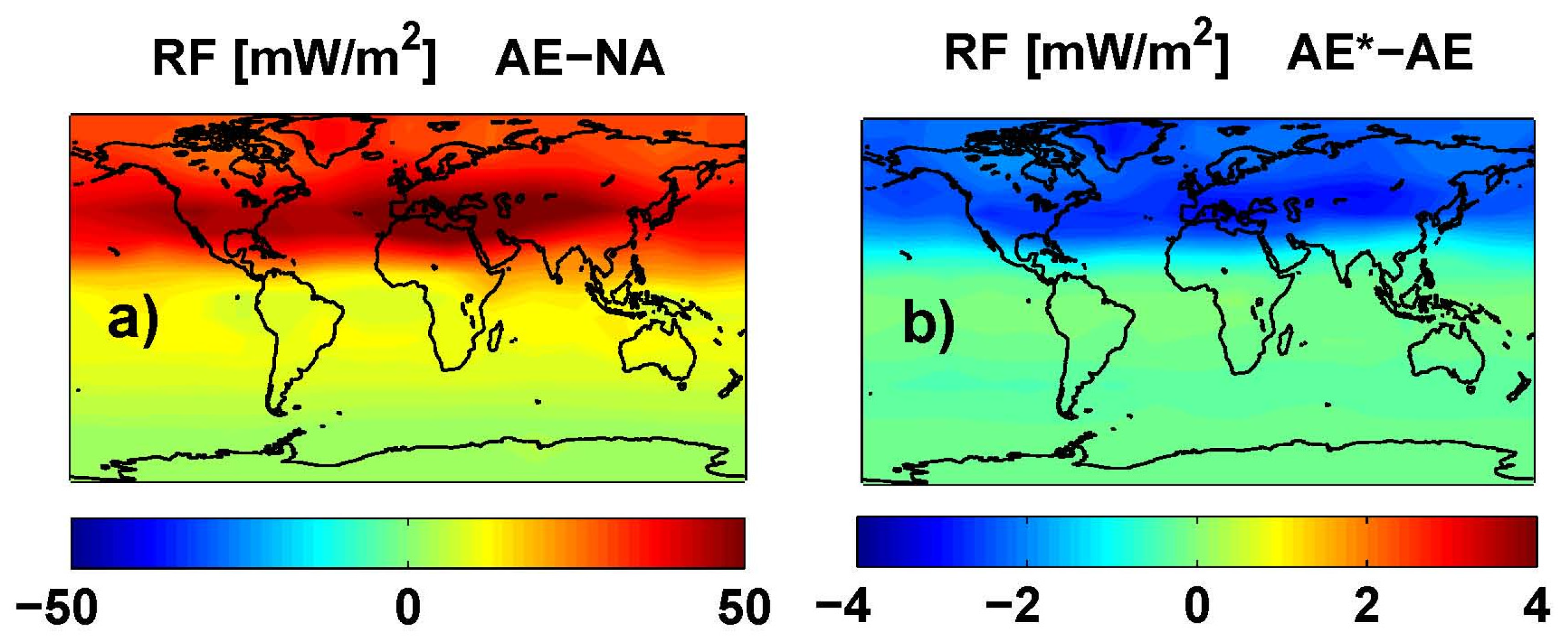
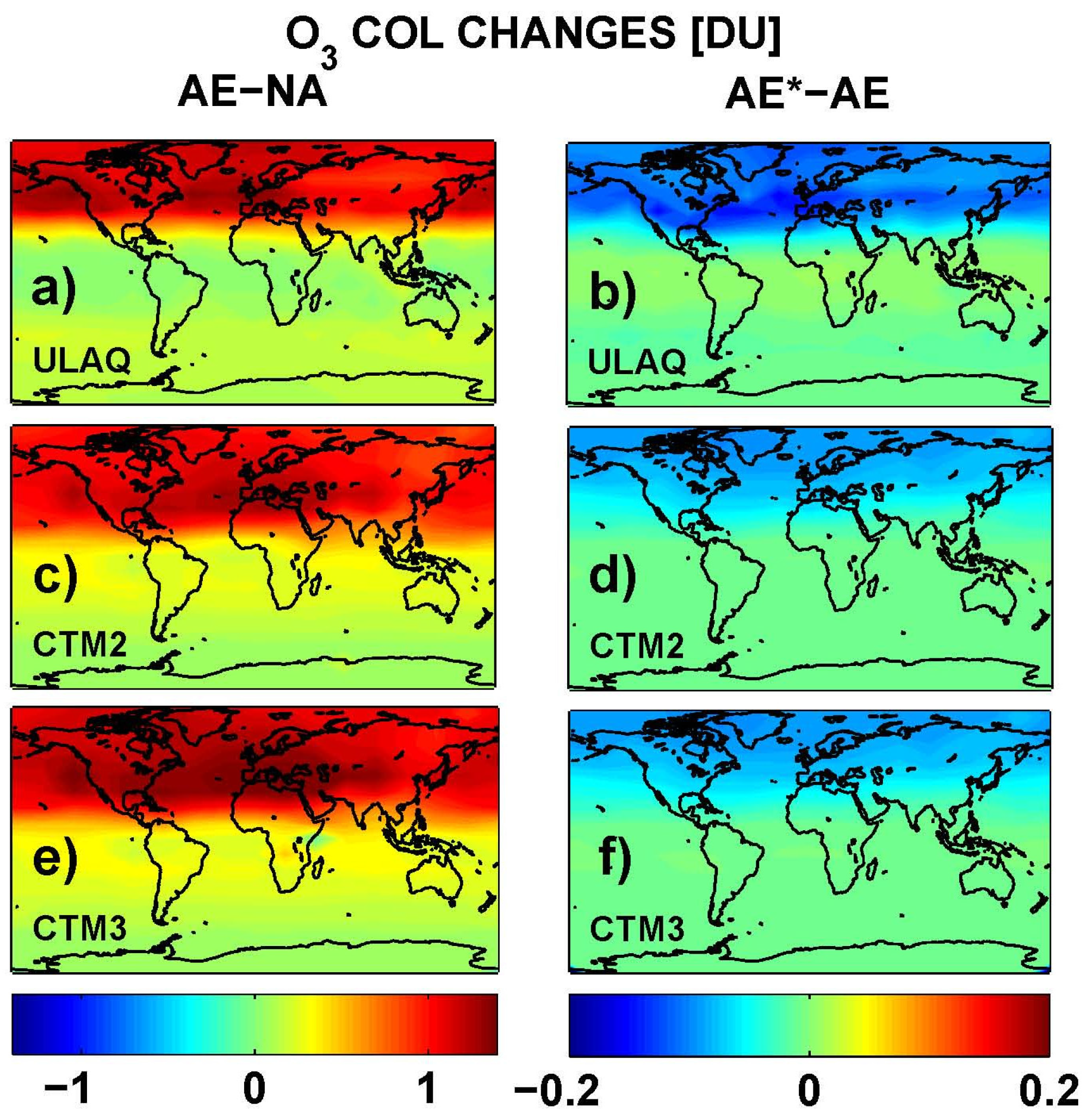
Latitude-longitude maps of the short-term O₃ RF are presented in Figure 11, in terms of average values over the three models (ULAQ, CTM2 and CTM3) and the two off-line radiative calculations (ULAQ, Oslo). Globally, the aviation aerosol effect on O₃ photochemistry is quantified as −4% of the aviation NO_x effect, in terms of radiative forcing. As expected, the geographical patterns of the calculated radiative forcing are closely linked to those of the ozone column changes in Figure 10.

Table 3. Summary of O₃ RF mean values for clear sky conditions. Differences are calculated between NA (experiment with no aircraft emission), AE (experiment with only gaseous emission [NO_x+H₂O]) and AE* (experiment with gaseous and particle emission [NO_x+H₂O+SO₄]). RF values are calculated with Oslo and ULAQ radiative code at ECMWF and National Center for Environmental Prediction (NCEP) tropopause level, respectively. LW, SW, NET are longwave, shortwave and net RFs, respectively. Only LW instantaneous values are considered here.

			Oslo			ULAQ
Model	EXP	O3 col [DU]	LW-inst [mW/m2]	SW [mW/m2]	NET-inst [mW/m2]	LW-inst [mW/m2]	SW [mW/m2]	NET-inst [mW/m2]
ULAQ	AE-NA	0.463	20.65	3.43	24.08	20.48	2.84	23.52
	AE*-NA	0.430	19.73	3.27	23.00	19.53	2.72	22.25
	AE*-AE	−0.033	−0.92	−0.16	−1.08	−0.95	−0.12	−1.07
CTM2	AE-NA	0.576	25.88	3.13	29.02	25.97	2.56	28.53
	AE*-NA	0.549	25.02	3.09	28.11	25.14	2.47	27.61
	AE*-AE	−0.026	−0.86	−0.04	−0.91	−0.83	−0.09	−0.92
CTM3	AE-NA	0.632	27.46	3.49	30.95	27.56	2.84	30.40
	AE*-NA	0.606	26.63	3.42	30.05	26.79	2.78	29.57
	AE*-AE	−0.026	−0.83	−0.07	−0.90	−0.77	−0.06	−0.83
ULAQ_FLX	AE-NA	0.264	14.12	3.52	17.64	14.10	2.93	17.03
	AE*-NA	0.251	13.66	3.37	17.03	13.64	2.84	16.48
	AE*-AE	−0.013	−0.46	−0.15	−0.61	−0.46	−0.09	−0.55

Table 3. Summary of O₃ RF mean values for clear sky conditions. Differences are calculated between NA (experiment with no aircraft emission), AE (experiment with only gaseous emission [NO_x+H₂O]) and AE* (experiment with gaseous and particle emission [NO_x+H₂O+SO₄]). RF values are calculated with Oslo and ULAQ radiative code at ECMWF and National Center for Environmental Prediction (NCEP) tropopause level, respectively. LW, SW, NET are longwave, shortwave and net RFs, respectively. Only LW instantaneous values are considered here.

			Oslo			ULAQ
Model	EXP	O3 col [DU]	LW-inst [mW/m2]	SW [mW/m2]	NET-inst [mW/m2]	LW-inst [mW/m2]	SW [mW/m2]	NET-inst [mW/m2]
ULAQ	AE-NA	0.463	20.65	3.43	24.08	20.48	2.84	23.52
	AE*-NA	0.430	19.73	3.27	23.00	19.53	2.72	22.25
	AE*-AE	−0.033	−0.92	−0.16	−1.08	−0.95	−0.12	−1.07
CTM2	AE-NA	0.576	25.88	3.13	29.02	25.97	2.56	28.53
	AE*-NA	0.549	25.02	3.09	28.11	25.14	2.47	27.61
	AE*-AE	−0.026	−0.86	−0.04	−0.91	−0.83	−0.09	−0.92
CTM3	AE-NA	0.632	27.46	3.49	30.95	27.56	2.84	30.40
	AE*-NA	0.606	26.63	3.42	30.05	26.79	2.78	29.57
	AE*-AE	−0.026	−0.83	−0.07	−0.90	−0.77	−0.06	−0.83
ULAQ_FLX	AE-NA	0.264	14.12	3.52	17.64	14.10	2.93	17.03
	AE*-NA	0.251	13.66	3.37	17.03	13.64	2.84	16.48
	AE*-AE	−0.013	−0.46	−0.15	−0.61	−0.46	−0.09	−0.55

Table 4. As in Table 3, but for total sky conditions. LW-RF and NET-RF with stratospheric temperature adjustment are also included here.

			Oslo				ULAQ
model	EXP	O3 col [DU]	LW-inst [mW/m2]	LW-adj [mW/m2]	SW [mW/m2]	NET-adj [mW/m2]	LW-inst [mW/m2]	LW-adj [mW/m2]	SW [mW/m2]	NET-adj [mW/m2]
ULAQ	AE-NA	0.463	14.82	12.59	5.26	17.85	16.43	13.64	4.52	18.16
	AE*-NA	0.430	14.16	12.03	5.02	17.05	15.72	13.03	4.32	17.35
	AE*-AE	−0.033	−0.66	−0.56	−0.24	−0.80	−0.71	−0.61	−0.20	−0.81
CTM2	AE-NA	0.576	18.70	16.19	4.75	20.94	21.65	17.99	4.01	22.00
	AE*-NA	0.549	18.06	15.50	4.63	20.13	20.95	17.26	3.89	21.15
	AE*-AE	−0.026	−0.64	−0.69	−0.12	−0.81	−0.70	−0.73	−0.12	−0.85
CTM3	AE-NA	0.632	19.77	17.11	5.27	22.38	22.80	19.16	4.44	23.60
	AE*-NA	0.606	19.18	16.59	5.14	21.63	22.25	18.52	4.35	22.87
	AE*-AE	−0.026	−0.59	−0.62	−0.13	−0.75	−0.64	−0.64	−0.09	−0.73
ULAQ_FLX	AE-NA	0.264	10.09	7.25	4.73	11.98	11.05	8.12	4.14	12.26
	AE*-NA	0.251	9.77	7.06	4.54	11.60	10.73	7.90	3.95	11.85
	AE*-AE	−0.013	−0.32	−0.19	−0.19	−0.38	−0.32	−0.22	−0.19	−0.41

Table 4. As in Table 3, but for total sky conditions. LW-RF and NET-RF with stratospheric temperature adjustment are also included here.

			Oslo				ULAQ
model	EXP	O3 col [DU]	LW-inst [mW/m2]	LW-adj [mW/m2]	SW [mW/m2]	NET-adj [mW/m2]	LW-inst [mW/m2]	LW-adj [mW/m2]	SW [mW/m2]	NET-adj [mW/m2]
ULAQ	AE-NA	0.463	14.82	12.59	5.26	17.85	16.43	13.64	4.52	18.16
	AE*-NA	0.430	14.16	12.03	5.02	17.05	15.72	13.03	4.32	17.35
	AE*-AE	−0.033	−0.66	−0.56	−0.24	−0.80	−0.71	−0.61	−0.20	−0.81
CTM2	AE-NA	0.576	18.70	16.19	4.75	20.94	21.65	17.99	4.01	22.00
	AE*-NA	0.549	18.06	15.50	4.63	20.13	20.95	17.26	3.89	21.15
	AE*-AE	−0.026	−0.64	−0.69	−0.12	−0.81	−0.70	−0.73	−0.12	−0.85
CTM3	AE-NA	0.632	19.77	17.11	5.27	22.38	22.80	19.16	4.44	23.60
	AE*-NA	0.606	19.18	16.59	5.14	21.63	22.25	18.52	4.35	22.87
	AE*-AE	−0.026	−0.59	−0.62	−0.13	−0.75	−0.64	−0.64	−0.09	−0.73
ULAQ_FLX	AE-NA	0.264	10.09	7.25	4.73	11.98	11.05	8.12	4.14	12.26
	AE*-NA	0.251	9.77	7.06	4.54	11.60	10.73	7.90	3.95	11.85
	AE*-AE	−0.013	−0.32	−0.19	−0.19	−0.38	−0.32	−0.22	−0.19	−0.41

Figure 11. O₃ RF (adjusted) (mW/m²) from an average of ULAQ, CTM2 and CTM3 model results and both radiative transfer codes. Left panel (a) is for AE-NA (globally averaged value: 20.82 mW/m²); right panel (b) is for AE*-AE (globally averaged value: −0.79 mW/m²).

Figure 11. O₃ RF (adjusted) (mW/m²) from an average of ULAQ, CTM2 and CTM3 model results and both radiative transfer codes. Left panel (a) is for AE-NA (globally averaged value: 20.82 mW/m²); right panel (b) is for AE*-AE (globally averaged value: −0.79 mW/m²).

A summary of the radiative forcing due to the aviation NO_x perturbation is presented in Table 5. We note that the short-term O₃ RF is close to, or slightly above, the mean value reported by Holmes et al. [5]. Further discussion on short-term O₃ RF from our models can be found in Søvde et al. [24]. Also listed in Table 5 is CH₄ radiative forcing. The latter is calculated as a function of the lifetime percentage reduction (∆τ-CH₄) due to the OH increase produced by the aircraft-induced NO_x increase (via NO + HO₂ → NO₂ + OH), with the following formula: CH₄-RF(mW/m²) = χ-CH₄(ppbv) × 0.37 × ∆τ-CH₄(%)/100 × 1.4 [77], where τ is the CH₄ lifetime. A magnification factor 1.4 is used to take into account that the CH₄ prediction in the models is usually made using a fixed mixing ratio boundary condition at the surface, so that the CH₄ adjustment to the upper tropospheric OH perturbation is underestimated. As explained in IPCC [85], the factor 1.4 may be used as a best estimate to adjust the calculated CH₄ lifetime change to the missing feedback of the upper tropospheric OH perturbation on the calculated lower tropospheric CH₄ mixing ratios. An exception to this is for the ULAQ_FLX experiment, where the CH₄ adjustment to the changing OH field is accounted for by the use of a flux boundary condition at the surface. Incidentally, we note that the ULAQ_FLX to ULAQ ratio of the CH₄ lifetime change is 1.39 for both AE-NA and AE*-NA, which is very close to the 1.4 factor suggested in IPCC [85].

The uncertainty in the calculated CH4 RF is estimated to be approximately ±10% [86], which would not significantly change our result. In the NO_x-related RF, we also include the effect of CH₄ on stratospheric water vapour. This is estimated to give an additional RF of 15% of the CH₄ RF [87], although the uncertainty is large, about 70% [86]. The CH₄ RF equation is a simplification of the detailed formula reported by IPCC [86]; those formulas are the basis for calculating the specific forcing, which is linked to the unperturbed CH₄ concentrations so that a higher CH₄ concentration yields a lower specific forcing. Our approach is often used when assessing impacts of small CH4 perturbations, and we find that our CH₄ RF differs by less than 1% compared to the full equations using CH₄ and N₂O. Scaling up our lifetime changes linearly to match 1 Tg(N)/year, we get about 1.1%–1.5%, which is in the lower range of Holmes et al. [5]. Gottschaldt et al. [23] finds a similar value of 1.5%, which is in agreement with our higher values. Correspondingly, our CH₄ RF is also in the lower range of Holmes et al. [5].

Table 5. Summary of NO_x-related RF mean value terms: O₃, CH₄ and PMO (primary mode ozone, i.e., long-term ozone response). Ozone RF values are obtained as a mean from Oslo and ULAQ radiative code calculations. Differences are calculated between NA (experiment with no aircraft emission), AE (experiment with only gaseous emission [NO_x+H₂O]) and AE* (experiment with gaseous and particle emission [NO_x+H₂O+SO₄]). See text for details on the calculations of CH₄ RF, PMO RF and the stratospheric H₂O RF induced by CH₄ changes. Note that for ULAQ_FLX, O₃-RF includes both short-term and long-term (primary mode) effects, whereas for the other models, only short-term O₃ RF is included (long-term effects are then included in “PMO RF”).

Species	EXP	ULAQ	CTM2	CTM3	ULAQ_FLX
ΔO3 col [DU]	AE-NA	0.463	0.576	0.632	0.264
	AE*-NA	0.430	0.549	0.606	0.251
	AE*-AE	−0.033	−0.026	−0.026	−0.013
O3 RF [mW/m2]	AE-NA	18.00	21.47	22.99	12.12
	AE*-NA	17.20	20.64	22.25	11.72
	AE*-AE	−0.80	−0.83	−0.74	−0.40
Δτ-CH4 [mo]	AE-NA	−0.82	−1.24	−1.13	−1.14
	AE*-NA	−0.76	−1.21	−1.09	−1.06
	AE*-AE	+0.06	+0.03	+0.04	+0.08
Δτ-CH4 [%]	AE-NA	−0.81	−1.03	−1.09	−1.17
	AE*-NA	−0.75	−1.01	−1.05	−1.09
	AE*-AE	+0.06	+0.02	+0.04	+0.08
CH4 RF [mW/m2]	AE-NA	−7.30	−9.33	−9.88	−7.60
	AE*-NA	−6.86	−9.14	−9.57	−7.08
	AE*-AE	+0.44	+0.18	+0.32	+0.52
Stratospheric H2O RF [mW/m2] from CH4 changes	AE-NA	−1.10	−1.40	−1.48	−1.14
	AE*-NA	−1.03	−1.37	−1.43	−1.06
	AE*-AE	+0.07	+0.03	+0.05	+0.08
PMO RF [mW/m2]	AE-NA	−3.65	−4.66	−4.94	–
	AE*-NA	−3.43	−4.57	−4.78	–
	AE*-AE	+0.22	+0.09	+0.16	--
TOTAL RF from NOx [mW/m2]	AE-NA	5.96	6.08	6.69	3.38
	AE*-NA	5.88	5.56	6.47	3.58
	AE*-AE	−0.08	−0.52	−0.22	+0.20

Table 5. Summary of NO_x-related RF mean value terms: O₃, CH₄ and PMO (primary mode ozone, i.e., long-term ozone response). Ozone RF values are obtained as a mean from Oslo and ULAQ radiative code calculations. Differences are calculated between NA (experiment with no aircraft emission), AE (experiment with only gaseous emission [NO_x+H₂O]) and AE* (experiment with gaseous and particle emission [NO_x+H₂O+SO₄]). See text for details on the calculations of CH₄ RF, PMO RF and the stratospheric H₂O RF induced by CH₄ changes. Note that for ULAQ_FLX, O₃-RF includes both short-term and long-term (primary mode) effects, whereas for the other models, only short-term O₃ RF is included (long-term effects are then included in “PMO RF”).

Species	EXP	ULAQ	CTM2	CTM3	ULAQ_FLX
ΔO3 col [DU]	AE-NA	0.463	0.576	0.632	0.264
	AE*-NA	0.430	0.549	0.606	0.251
	AE*-AE	−0.033	−0.026	−0.026	−0.013
O3 RF [mW/m2]	AE-NA	18.00	21.47	22.99	12.12
	AE*-NA	17.20	20.64	22.25	11.72
	AE*-AE	−0.80	−0.83	−0.74	−0.40
Δτ-CH4 [mo]	AE-NA	−0.82	−1.24	−1.13	−1.14
	AE*-NA	−0.76	−1.21	−1.09	−1.06
	AE*-AE	+0.06	+0.03	+0.04	+0.08
Δτ-CH4 [%]	AE-NA	−0.81	−1.03	−1.09	−1.17
	AE*-NA	−0.75	−1.01	−1.05	−1.09
	AE*-AE	+0.06	+0.02	+0.04	+0.08
CH4 RF [mW/m2]	AE-NA	−7.30	−9.33	−9.88	−7.60
	AE*-NA	−6.86	−9.14	−9.57	−7.08
	AE*-AE	+0.44	+0.18	+0.32	+0.52
Stratospheric H2O RF [mW/m2] from CH4 changes	AE-NA	−1.10	−1.40	−1.48	−1.14
	AE*-NA	−1.03	−1.37	−1.43	−1.06
	AE*-AE	+0.07	+0.03	+0.05	+0.08
PMO RF [mW/m2]	AE-NA	−3.65	−4.66	−4.94	–
	AE*-NA	−3.43	−4.57	−4.78	–
	AE*-AE	+0.22	+0.09	+0.16	--
TOTAL RF from NOx [mW/m2]	AE-NA	5.96	6.08	6.69	3.38
	AE*-NA	5.88	5.56	6.47	3.58
	AE*-AE	−0.08	−0.52	−0.22	+0.20

Ozone changes produced by tropospheric NO_x emissions are not only associated with a short-term response of the NO_x and HO_x perturbations (see Table 3 and Table 4). The long-term response to CH₄ changes driven by the OH perturbation has to be considered as well. As discussed above, CTMs are normally run using a fixed mixing ratio boundary condition at the surface and this does not allow lower tropospheric CH₄ to adjust to the upper tropospheric OH perturbation produced by aviation NO_x emissions. In this case, a parametric formula, such as the one adopted here, i.e., PMO-RF = 0.5 × CH₄-RF [86], has to be used in order to estimate the long-term “primary mode” effect. The O₃ RF reported in Table 5 for ULAQ_FLX includes both the short-and long-term responses of ozone. The difference between ULAQ and ULAQ_FLX represents in a first approximation the long-term O₃ response in ULAQ_FLX, which is approximately 77% of the ULAQ_FLX CH₄-RF. This is a larger value with respect to the 50% used in the parametric formula above, simply because the calculated difference between ULAQ and ULAQ_FLX in the short-term O₃ RF includes not only the PMO RF, but also the feedback in ULAQ_FLX of the changing CH₄ on stratospheric water vapour and finally on HO_x and NO_x catalytic cycles for ozone destruction.

A summary of the RF from aviation aerosol is presented in Table 6. The calculated normalized direct forcings for sulphate and BC (−140 and 1700 W/g, respectively) are comparable with those reported in IPCC [85] (i.e., −125 to −214 and 1100–3000 W/g, respectively). The BC RF (+0.8 mW/m², globally) is due to direct soot emission from the aircraft (with an effective radius of 0.14 μm). The sulphate RF (−3.5 mW/m², globally) is due to aircraft emissions of SO₂ (EI = 0.8 g-SO₂/kg-fuel), which is oxidized by OH to SO₄ with additional condensation in the accumulation mode of the sulphate aerosol size distribution (with a calculated effective radius of 0.16 μm). The RF signs of BC (positive) and SO₄ (negative) are due to the dominant solar radiation absorption and scattering, respectively. The indirect RF of aviation soot through formation of upper tropospheric cirrus-ice particles via heterogeneous freezing (i.e., the soot-cirrus RF) is obtained on the basis of a particle size distribution with a calculated effective radius of 5 μm (+4.9 mW/m², globally). The largest uncertainty on this soot-cirrus RF comes from the BC fraction assumed to act as ice nuclei (0.1% in our case). Values in the range 0.1%–1.0% (or even smaller) are suggested by Hendricks et al. [68]. For soot-cirrus, the longwave contribution dominates over the shortwave forcing, due to the size of these particles, whereas for BC and SO₄ the solar forcing dominates. Table 7 shows that the indirect BC results are consistent with Gettelman and Chen [20], where an aviation impact <10 mW/m² was observed when a fixed nucleating efficiency of 0.1% for BC was applied. Furthermore, the RFs per unit BC emission from both studies are within 2.5% of each other. However, it should be noted that the treatment of background ice nucleation, together with the uncertainties in the ice nucleation potential of “pre-activated” aircraft soot, could produce large uncertainties surrounding the indirect effect of aircraft soot, resulting in either negative or positive RF, as shown by Zhou and Penner [88] and also summarized in Table 7.

Table 8 presents an overall summary of the aviation RFs calculated in the present study, excluding CO₂, contrails and contrail-cirrus, which are not explicitly considered in the present study. The contribution of aviation water vapour accumulating above the tropopause is also considered, and the calculated value (0.6 mW/m²) is consistent with that obtained and discussed in Wilcox et al. [89] (0.9 ± 0.5 mW/m²). According to our calculations, aircraft emitted aerosols tend to decrease the O₃ production and its positive RF (by −0.27±0.2 mW/m²), but on the other hand the net contribution of direct and indirect soot forcings (positive) plus the direct sulphate forcing (negative) (+2.7 mW/m²) tends to increase the overall aviation RF. The small and negative SO4 forcing (−0.2 mW/m²) in the AE-NA case is due to the OH increase produced by aviation NO_x emissions, which favours the SO₂ oxidation into sulphate. According to our calculations, the net NO_x-induced RF appears to be the dominant term (excluding CO₂ and contrails), although it might be somewhat overestimated, because the effect of NOx emissions on nitrate aerosols is not included in this study. However, the existence of such an effect (from aviation emissions) and its magnitude are not well established. An increasing contribution to solar radiation scattering would add a negative term to the NO_x-related RF, as demonstrated by Unger et al. [90]. However, there are not enough studies whereby nitrates are included in CTM simulations and therefore, a reliable RF estimate that is comparable to the rest of the aviation RFs reported in the study is not available. In addition, a rather marginal effect of aircraft emissions on nitrate aerosol could be expected when taking into account that the formation of nitrate aerosols (NH4⁺NO3⁻) requires a significant presence of ammonium, which may be the case only in the lower troposphere. Holmes et al. [5] have shown a net NO_x effect amounting to 4.5 ± 4.5 mW/m² for 1 Tg(N)/year aircraft emissions. Our results are consistent with that estimate.

Table 6. Summary of aerosol Radiative Forcing mean values: direct contributions from sulphate and soot (BC) and indirect BC forcing (soot-cirrus) (AE*-NA): ULAQ-CTM values and ULAQ radiative code. Here Δτ is the particle optical thickness perturbation at λ = 0.55 μm. The final column shows the normalized RF (i.e., absolute value of the net-RF divided by the globally averaged Δ-load).

Species	Δ-load TOT [μg/m2]	Δ-load STRAT [μg/m2]	Δτ [λ = 0.55 μm]	SW [mW/m2]	LW-inst [mW/m2]	LW-adj [mW/m2]	NET-adj [mW/m2]	NRF [W/g]
SO4	25.0	6.6	2.4E-04	−5.2	1.8	1.7	−3.5	140
BC	0.46	0.10	3.0E-06	0.85	0.01	−0.08	0.78	1700
Soot Cirrus	320	0	1.0E-04	−1.7	6.6	6.6	4.9	15

Table 6. Summary of aerosol Radiative Forcing mean values: direct contributions from sulphate and soot (BC) and indirect BC forcing (soot-cirrus) (AE*-NA): ULAQ-CTM values and ULAQ radiative code. Here Δτ is the particle optical thickness perturbation at λ = 0.55 μm. The final column shows the normalized RF (i.e., absolute value of the net-RF divided by the globally averaged Δ-load).

Species	Δ-load TOT [μg/m2]	Δ-load STRAT [μg/m2]	Δτ [λ = 0.55 μm]	SW [mW/m2]	LW-inst [mW/m2]	LW-adj [mW/m2]	NET-adj [mW/m2]	NRF [W/g]
SO4	25.0	6.6	2.4E-04	−5.2	1.8	1.7	−3.5	140
BC	0.46	0.10	3.0E-06	0.85	0.01	−0.08	0.78	1700
Soot Cirrus	320	0	1.0E-04	−1.7	6.6	6.6	4.9	15

Table 7. RF from other soot-cirrus studies. Relevant experiments not directly comparable to this study are also included for illustrative purposes.

	This study	Gettelman and Chen [20]	Zhou and Penner [88]
Model	ULAQ-CTM	CAM5/MAM	CAM5.2/IMPACT
Experimental setup	Fixed nucleating efficiency (0.1%), with aviation NOx and SO4, no contrails.	Fixed nucleating efficiency (0.1%), no aviation NOx/SO4/contrails. [Also with SO4 and contrails]	[Varying nucleating efficiencies to include pre-activated soot and sensitivity to background. No aviation NOx, with contrails]
Aircraft BC emission (Tg-BC/year)	0.00407	0.00681	0.00681
Soot-cirrus TOA RF (mW/m2)	4.9	8.0 [−21 ± 11]	[−350 to 90]
RF per unit BC emission (Wm−2/Tg-BC/year)	1.20	1.17

Table 7. RF from other soot-cirrus studies. Relevant experiments not directly comparable to this study are also included for illustrative purposes.

	This study	Gettelman and Chen [20]	Zhou and Penner [88]
Model	ULAQ-CTM	CAM5/MAM	CAM5.2/IMPACT
Experimental setup	Fixed nucleating efficiency (0.1%), with aviation NOx and SO4, no contrails.	Fixed nucleating efficiency (0.1%), no aviation NOx/SO4/contrails. [Also with SO4 and contrails]	[Varying nucleating efficiencies to include pre-activated soot and sensitivity to background. No aviation NOx, with contrails]
Aircraft BC emission (Tg-BC/year)	0.00407	0.00681	0.00681
Soot-cirrus TOA RF (mW/m2)	4.9	8.0 [−21 ± 11]	[−350 to 90]
RF per unit BC emission (Wm−2/Tg-BC/year)	1.20	1.17

Table 8. Summary of Radiative Forcing (RF) mean values relevant for aviation emissions, excluding CO₂, contrails and contrail-cirrus, which are not explicitly considered in the present study. RF values from NO_x are obtained as a mean from the CTMs (ULAQ, CTM2 and CTM3) and Oslo and ULAQ radiative code calculations. The uncertainty interval is calculated as the range of the net NO_x-related RF from the three models.

species	RF [mW/m2] AE-NA	RF [mW/m2] AE*-NA	RF [mW/m2] AE*-AE
TOTAL RF from NOx	6.2 ± 0.4	6.0 ± 0.4	−0.27 ± 0.2
Direct SO4 RF	−0.2	−3.5	−3.3
Direct BC RF	0.0	0.8	0.8
Indirect BC RF (soot cirrus)	0.0	4.9	4.9
Stratospheric H2O	0.6	0.6	0.0
TOTAL RF	6.6	8.8	2.2

Table 8. Summary of Radiative Forcing (RF) mean values relevant for aviation emissions, excluding CO₂, contrails and contrail-cirrus, which are not explicitly considered in the present study. RF values from NO_x are obtained as a mean from the CTMs (ULAQ, CTM2 and CTM3) and Oslo and ULAQ radiative code calculations. The uncertainty interval is calculated as the range of the net NO_x-related RF from the three models.

species	RF [mW/m2] AE-NA	RF [mW/m2] AE*-NA	RF [mW/m2] AE*-AE
TOTAL RF from NOx	6.2 ± 0.4	6.0 ± 0.4	−0.27 ± 0.2
Direct SO4 RF	−0.2	−3.5	−3.3
Direct BC RF	0.0	0.8	0.8
Indirect BC RF (soot cirrus)	0.0	4.9	4.9
Stratospheric H2O	0.6	0.6	0.0
TOTAL RF	6.6	8.8	2.2

4. Conclusions

In this work, we have estimated the effect of aircraft gaseous and particulate sulphur emissions in three CTMs, the ULAQ-CTM, Oslo CTM3 and Oslo CTM2. The surface area densities of sulphate aerosols were calculated on-line by the ULAQ-CTM, and were included as monthly means in the Oslo CTMs because of their lack of aerosol modules capable of handling aircraft aerosols. Aerosol mass prediction with the ULAQ-CTM has been widely validated through the participation in international inter-comparison projects, but was also validated here. The model performed well in reproducing observed aerosol mass concentrations, with discrepancies in a few South Atlantic observational sites, which could be attributed to the inefficient parameterization of removal processes. The processing of emission sources towards an altitudinal distribution of aerosol mass involves sulphate chemistry, transport and removal processes. These mechanisms have a large potential for errors, so they have to be controlled by the optical depth validation and extinction simulated values. Optical thickness has been validated by means of SAGE-II measurements and AVHRR, TOMS and MODIS retrievals; with the ULAQ model reproducing the seasonal variation for both oceanic and land regions of the North Atlantic. Moreover, the ULAQ model performed well when compared with SAGE-II data. While analysing the contribution to extinction from different aerosol types, sulphate aerosols gave the largest contribution at the tropopause height. We found that the inclusion of aircraft sulphur and aerosols emissions produced a slightly smaller impact on O₃ than when only aircraft NO_x emissions were considered. According to our calculations, this changed the net O₃-RF (i.e., short- and long-term O₃ RF) by −0.63 mW/m² (i.e., −3.8%). A change in OH will also set up a small increase in CH₄ and its RF, which we found to be +0.36 mW/m² (i.e., +3.5%) and this includes also the CH₄ feedback on stratospheric water vapour. The calculated aerosol-driven net change of the NO_x-related RF produced by aircraft emissions of sulphate aerosols accounts then for −0.27 mW/m² (i.e., −4.4%)

The long-term response to CH₄ changes due to aviation NO_x emissions were also considered in this study. In the ULAQ_FLX experiment, using a CH₄ surface flux boundary condition, we find a long-term impact on O₃ amounting to 77% of the CH₄ RF. This is near the upper limit of the IPCC recommended range of values, when taking into account a 55% uncertainty for the PMO. Our larger number originates from the feedback of the changing CH₄ on stratospheric water vapour and finally on HO_x and NO_x catalytic cycles for stratospheric ozone destruction.

The RF from direct SO₄ and BC were found to be −3.3 mW/m² and +0.8 mW/m², respectively, while the indirect BC result (soot-cirrus) was estimated to be +4.9 mW/m². The direct effects were comparable to other studies. As for soot-cirrus, there are still large uncertainties surrounding the estimate, not just in terms of its magnitude but also whether it has a warming or cooling effect. This study shows that aerosols should be included in model simulations, with the largest aerosol impacts seen in the indirect effects of BC on clouds and not their effects on NO_x chemistry (excluding the effect of nitrates). However, further work is necessary to quantify these indirect effects and their sensitivities to parameters such as background sulphate concentrations and the interaction between aviation aerosols and contrails-cirrus.

References

1. Sausen, R.; Isaksen, I.; Grewe, V.; Hauglustaine, D.; Lee, D.S.; Myhre, G.; Köhler, M.O.; Pitari, G.; Schumann, U.; Stordal, F.; Zerefos, C. Aviation radiative forcing in 2000: An update on IPCC (1999). Meteorol. Z. 2005, 14, 555–561. [Google Scholar]
2. Lee, D.S.; Pitari, G.; Grewe, V.; Gierens, K.; Penner, J.; Petzold, A.; Prather, M.; Schumann, U.; Bais, A.; Berntsen, T.; et al. Transport impacts on atmosphere and climate: Aviation. Atmos. Environ. 2010, 44, 4678–4734. [Google Scholar] [CrossRef]
3. Köhler, M.O.; Rädel, G.; Dessens, O.; Shine, K.P.; Rogers, H.L.; Wild, O.; Pyle, J.A. Impact of perturbations to nitrogen oxide emissions from global aviation. J. Geophys. Res. 2008, 113, D11305. [Google Scholar] [CrossRef]
4. Hoor, P.; Borken-Kleefeld, J.; Caro, D.; Dessens, O.; Endresen, O.; Gauss, M.; Grewe, V.; Hauglustaine, D.; Isaksen, I.S.A.; Jöckel, P.; et al. The impact of traffic emissions on atmospheric ozone and OH: results from QUANTIFY. Atmos. Chem. Phys. 2009, 9, 3113–3136. [Google Scholar] [CrossRef]
5. Holmes, C.D.; Tang, Q.; Prather, M.J. Uncertainties in climate assessment for the case of aviation NO. P. Natl. Acad. Sci. USA 2011, 108, 10997–11002. [Google Scholar] [CrossRef] [PubMed]
6. Kraabøl, A.G.; Berntsen, T.K.; Sundet, J.K.; Stordal, F. Impacts of NOx emissions from subsonic aircraft in a global three-dimensional chemistry transport model including plume processes. J. Geophys. Res. 2002, 107. [Google Scholar] [CrossRef]
7. Cariolle, D.; Caro, D.; Paoli, R.; Hauglustaine, D.A.; Cuénot, B.; Cozic, A.; Paugam, R. Parameterization of plume chemistry into large-scale atmospheric models: Application to aircraft NOx emissions. J. Geophys. Res. 2009, 114, D19302. [Google Scholar] [CrossRef]
8. Weisenstein, D.; Ko, M.; Dyominov, I.; Pitari, G.; Ricciardulli, L.; Visconti, G.; Bekki, S. The effects of sulfur emissions from HSCT aircraft: a 2-D model intercomparison. J. Geophys. Res. 1998, 103, 1527–1547. [Google Scholar] [CrossRef]
9. Pitari, G.; Mancini, E.; Bregman, A. Climate forcing of subsonic aviation: indirect role of sulfate particles via heterogeneous chemistry. Geophys. Res. Lett. 2002, 29. [Google Scholar] [CrossRef]
10. Søvde, O.A.; Gauss, M.; Isaksen, I.S.A.; Pitari, G.; Marizy, C. Aircraft pollution—A futuristic view. Atmos. Chem Phys. 2007, 7, 3621–3632. [Google Scholar] [CrossRef]
11. Hendricks, J.; Kärcher, B.; Lohmann, U.; Ponater, M. Do aircraft black carbon emissions affect cirrus clouds on the global scale? Geophys. Res. Lett. 2005, 32, L12814. [Google Scholar] [CrossRef]
12. Burkhardt, U.; Kärcher, B. Global radiative forcing from contrail cirrus. Nat. Clim. Chang. 2011, 1, 54–58. [Google Scholar] [CrossRef]
13. Meilinger, S.K.; Kärcher, B.; Peter, T. Suppression of chlorine activation on aviation-produced volatile particles. Atmos. Chem. Phys. 2002, 2, 307–312. [Google Scholar] [CrossRef]
14. Sander, S.P.; Friedl, R.R.; Barker, J.R.; Golden, D.M.; Kurylo, M.J.; Wine, P.H.; Abbatt, J.P.D.; Burkholder, J.B.; Kolb, C.E.; Moortgat, G.K.; et al. Chemical Kinetics and Photochemical Data for Use in Atmospheric Studies, Evaluation No. 17; Tech. Rep. 10–06; California Institute of Technology: Pasadena, CA, USA, 2011. [Google Scholar]
15. Pueschel, R.F.; Hallett, J.; Strawa, A.W.; Howard, S.D.; Ferry, G.V.; Foster, T.; Arnott, W.P. Aerosol and cloud particles in tropical cirrus anvil: importance to radiation balance. J. Aerosol. Sci. 1997, 28, 1123–1136. [Google Scholar] [CrossRef]
16. Curtius, J.; Sierau, B.; Arnold, F.; Baumann, R.; Busen, R.; Schulte, P.; Schumann, U. First direct sulfuric acid detection in the exhaust plume of a jet aircraft in flight. Geophys. Res. Lett. 1998, 25, 923–926. [Google Scholar] [CrossRef]
17. Kärcher, B.; Meilinger, S.K. Perturbation of the aerosol layer by aviation-produced aerosols: A parameterization of plume processes. Geophys. Res. Lett. 1998, 25, 4465–4468. [Google Scholar] [CrossRef]
18. Fahey, D.W.; Keim, E.R.; Woodbridge, E.L.; Gao, R.S.; Boering, K.A.; Daube, B.C.; Wofsy, S.C.; Lohmann, R.P.; Hinsta, E.J.; Lowenstein, M.; et al. In situ observations in aircraft exhaust plumes in the lower stratosphere at midlatitudes. J. Geophys. Res. 1995, 100, 3065–3074. [Google Scholar] [CrossRef]
19. Kärcher, B.; Lohmann, U. A parameterization of cirrus cloud formation: homogeneous freezing of supercooled aerosols. J. Geophys. Res. 2002, 107. [Google Scholar] [CrossRef]
20. Gettelman, A.; Chen, C. The climate impact of aviation aerosols. Geophys. Res. Lett. 2013, 40, 1–5. [Google Scholar] [CrossRef]
21. Unger, N. Global climate impact of civil aviation for standard and desulfurized jet fuel. Geophys. Res. Lett. 2011, 38, L20803. [Google Scholar] [CrossRef]
22. Grewe, V.; Tsati, E.; Hoor, P. On the attribution of contributions of atmospheric trace gases to emissions in atmospheric model applications. Geosci. Model Dev. 2010, 3, 487–499. [Google Scholar] [CrossRef] [Green Version]
23. Gottschaldt, K.; Voigt, C.; Jöckel, P.; Righi, M.; Deckert, R.; Dietmüller, S. Global sensitivity of aviation NOx effects to the HNO3-forming channel of the HO2 + NO reaction. Atmos. Chem. Phys. 2013, 13, 3003–3025. [Google Scholar] [CrossRef]
24. Søvde, O.A.; Matthes, S.; Skowron, A.; Iachetti, D.; Lim, L.; Hodnebrog, Ø.; Di Genova, G.; Pitari, G.; Lee, D.S.; Myhre, G.; Isaksen, I.S.A. Aircraft emission mitigation by changing route altitude: A multi-model estimate of aircraft NOx emission impact on O3 photochemistry. Atmos. Environ. 2014. [Google Scholar] [CrossRef]
25. Pitari, G.; Mancini, E.; Rizi, V.; Shindell, D.T. Impact of future climate and emission changes on stratospheric aerosols and ozone. J. Atmos. Sci. 2002, 59, 414–440. [Google Scholar] [CrossRef]
26. Eyring, V.; Butchart, N.; Waugh, D.W.; Akiyoshi, H.; Austin, J.; Bekki, S.; Bodeker, G.E.; Boville, B.A.; Bruhl, C.; Chipperfield, M.P.; et al. Assessment of temperature, trace species, and ozone in chemistry-climate model simulation of the recent past. J. Geophys. Res. 2006, 99, D22308. [Google Scholar] [CrossRef]
27. Morgenstern, O.; Giorgetta, M.A.; Shibata, K.; Eyring, V.; Waugh, D.W.; Shepherd, T.G.; Akiyoshi, H.; Austin, J.; Baumgärtner, A.; Bekki, S.; et al. A review of CCMVal-2 models and simulations. J. Geophys. Res. 2010, 115, D00M02. [Google Scholar]
28. Pitari, G.; Aquila, V.; Kravitz, B.; Robock, A.; Watanabe, S.; Cionni, I.; De Luca, N.; Di Genova, G.; Mancini, E.; Tilmes, S. Stratospheric Ozone Response to Sulfate Geoengineering: Results from the Geoengineering Model Intercomparison Project (GeoMIP). J. Geophys. Res. 2014, 119, 2629–2653. [Google Scholar] [CrossRef]
29. Minschwaner, K.; Salawitch, R.J.; McElroy, M.B. Absorption of Solar Radiation by O2: Implications for O3 and Lifetimes of N2O, CFCl3, and CF2Cl2. J. Geophys. Res. 1993, 98, 543–561. [Google Scholar]
30. Rayner, N.A.; Parker, D.E.; Horton, E.B.; Folland, C.K.; Alexander, L.V.; Rowell, D.P.; Kent, E.C.; Kaplan, A. Global analyses of sea surface temperature, sea ice, and night marine air temperature since the late nineteenth century. J. Geophys. Res. 2003, 108. [Google Scholar] [CrossRef] [Green Version]
31. Pitari, G.; Rizi, V.; Ricciardulli, L.; Visconti, G. High-Speed civil transport impact: The role of Sulfate, Nitric acid Trihydrate and ice aerosols studied with a two-dimensional model including aerosol physics. J. Geophys. Res. 1993, 98. [Google Scholar] [CrossRef]
32. Brunner, D.; Staehelin, J.; Rogers, H.L.; Köhler, M.O.; Pyle, J.A.; Hauglustaine, D.; Jourdain, L.; Berntsen, T.K.; Gauss, M.; Isaksen, I.S.A.; Meijer, E.; et al. An evaluation of the performance of chemistry transport models—Part 2: Detailed comparison with two selected campaigns. Atmos. Chem. Phys. 2005, 5, 107–129. [Google Scholar] [CrossRef]
33. Chou, M.-D.; Suarez, M.J.; Liang, X.-Z. A Thermal Infrared Radiation Parameterization for Atmospheric Studies; NASA Goddard Space Flight Center: Greenbelt, MD, USA, 2001; p. 55. [Google Scholar]
34. Søvde, O.A.; Prather, M.J.; Isaksen, I.S.A.; Berntsen, T.K.; Stordal, F.; Zhu, X.; Holmes, C.D.; Hsu, J. The chemical transport model Oslo CTM3. Geosci. Model Dev. 2012, 5, 1441–1469. [Google Scholar] [CrossRef]
35. Prather, M.J.; Zhu, X.; Strahan, S.E.; Steenrod, S.D.; Rodriguez, J.M. Quantifying errors in trace species transport modeling. Proc. Natl. Acad. Sci. USA 2008, 105, 19617–19621. [Google Scholar] [CrossRef] [PubMed]
36. Holtslag, A.A.M.; DeBruijn, E.I.F.; Pan, H.L. A high resolution air mass transformation model for short-range weather forecasting. Mon. Wea. Rev. 1990, 118, 1561–1575. [Google Scholar] [CrossRef]
37. Berntsen, T.; Isaksen, I.S.A. A global 3-D chemical transport model for the troposphere, Model description and CO and Ozone results. J. Geophys. Res. 1997, 102, 21239–21280. [Google Scholar] [CrossRef]
38. Berglen, T.F.; Berntsen, T.K.; Isaksen, I.S.A.; Sundet, J.K. A global model of the coupled sulfur/oxidant chemistry in the troposphere: The sulfur cycle. J. Geophys. Res. 2004, 109, D19310. [Google Scholar] [CrossRef]
39. Søvde, O.A.; Gauss, M.; Smyshlyaev, S.P.; Isaksen, I.S.A. Evaluation of the chemical transport model Oslo CTM2 with focus on Arctic winter ozone depletion. J. Geophys. Res. 2008, 113, D09304. [Google Scholar]
40. Hesstvedt, E.; Hov, O.; Isaksen, I.S.A. Quasi steady-state approximation in air pollution modelling: Comparison of two numerical schemes for oxidant prediction. Int. J. Chem. Kin. 1978, X, 971–994. [Google Scholar] [CrossRef]
41. Søvde, O.A.; Hoyle, C.R.; Myhre, G.; Isaksen, I.S.A. The HNO3 forming branch of the HO2 + NO reaction: preindustrial-to-present trends in atmospheric species and radiative forcings. Atmos. Chem. Phys. 2011, 11, 8929–8943. [Google Scholar] [CrossRef]
42. Prather, M.J. Numerical advection by conservation of second-order moments. J. Geophys. Res. 1986, 91, 6671–6681. [Google Scholar] [CrossRef]
43. Price, C.; Penner, J.; Prather, M. NOx from lightning 1. Global distribution based on lightning physics. J. Geophys. Res. 1997, 102, 5929–5941. [Google Scholar] [CrossRef]
44. Berntsen, T.K.; Isaksen, I.S.A. Effects of lightning and convection on changes in upper tropospheric ozone due to NOx emissions from aircraft. Tellus 1999, 51, 766–788. [Google Scholar] [CrossRef]
45. Ott, L.E.; Pickering, K.E.; Stenchikov, G.L.; Allen, D.J.; De Caria, A.J.; Ridley, B.; Lin, R.-F.; Lang, S.; Tao, W.K. Production of lightning NOx and its vertical distribution calculated from three-dimensional cloud-scale chemical transport model simulations. J. Geophys. Res. 2010, 115, D04301. [Google Scholar]
46. Pickering, K.E.; Wang, Y.S.; Tao, W.K.; Price, C.; Muller, J.F. Vertical distributions of lightning NOx for use in regional and global chemical transport models. J. Geophys. Res. 1998, 103, 31203–31216. [Google Scholar] [CrossRef]
47. Lee, D.S.; Owen, B.; Fichter, C.; Lim, L.L.; Dimitriu, D. Allocation of International Aviation Emissions from Scheduled Air Traffic - Present Day and Historical (Report 2 of 3); Final Report to the UK Department for Environment, Food and Rural Affairs(DEFRA) Global Atmosphere Division; Manchester Metropolitan University: Manchester, UK, 2005. [Google Scholar]
48. Lee, D.S.; Fahey, D.W.; Forster, P.M.; Newton, P.J.; Wit, R.C.N.; Lim, L.L.; Owen, B.; Sausen, R. Aviation and global climate change in the 21st century. Atmos. Environ. 2009, 43, 3520–3537. [Google Scholar] [CrossRef]
49. Owen, B.; Lee, D.S.; Lim, L.L. Flying into the future: Aviation emissions scenarios to 2050. Environ. Sci. Technol. 2010, 44, 2255–2260. [Google Scholar] [CrossRef] [PubMed]
50. ICAO. International Civil Aviation Organization. 2013. Available online: http://www.icao.int/environmental-protection/Pages/modelling-and-databases.aspx (accessed on 29 May 2015).
51. ICAO/CAEP. International Civil Aviation Organization (ICAO)/Committee on Aviation Environmental Protection (CAEP), Agenda Item 4: Modeling and Databases Task Force (MODTF) goals assessment results. In Proceedings of the ICAO/CAEP Working Paper, Steering Group Meeting, Salvador, Brazil, 22–26 June 2009.
52. Simos, D. PIANO User’s Guide Version 5.0; Lissys Limited: Loughborough, UK, 2008; Available online: www.piano.aero (accessed on 29 May 2015).
53. Eyers, C.J.; Norman, P.; Middel, J.; Plohr, M.; Michot, S.; Atkinson, K.; Christou, R.A. AERO2k Global Aviation Emissions Inventories for 2002 and 2025. QINETIQ/04/01113. QINETIQ Ltd.: Hampshire, UK, December 2004. Available online: http://aero-net.info/fileadmin/aeronet_files/links/documents/AERO2K_Global_Aviation_Emissions_Inventories_for_2002_and_2025.pdf (accessed on 29 May 2015).
54. Barrett, S.; Prather, M.; Penner, J.; Selkirk, H.; Balasubramanian, S.; Dopelheuer, A.; Fleming, G.; Gupta, M.; Halthore, R.; Hileman, J.; et al. Guidance on the use of AEDT Gridded Aircraft Emissions in Atmospheric Models, Version 2.0; Technical Note LAE-2010-008-N. US Federal Aviation Administration: Washington, DC, USA, August 2010. Available online: http://lae.mit.edu/uploads/LAE_report_series/2010/LAE-2010-008-N.pdf (accessed on 29 May 2015).
55. Penner, J.E.; Hegg, D.; Andreae, M.; Leaitch, D.; Pitari, G.; Annegarn, H.; Murphy, D.; Nganga, J.; Barrie, L.; Feichter, H. Aerosols and Indirect Cloud Effects, IPCC Third assessment report. In IPCC Climate Change 2001; Cambridge University Press: Cambridge, UK, 2001; pp. 289–348. [Google Scholar]
56. Koch, D.; Schulz, M.; Kinne, S.; Schuster, G.; Bond, T.C.; Clarke, A.; Fahey, D.W.; Freitag, S.; McNaughton, C.; Spackman, J.R.; et al. Evaluation of black carbon estimations in global aerosol models. Atmos. Chem. Phys. 2009, 9, 9001–9026. [Google Scholar] [CrossRef]
57. Bond, T.C.; Doherty, S.J.; Fahey, D.W.; Forster, P.M.; Berntsen, T.; DeAngelo, B.J.; Flanner, M.G.; Ghan, S.; Kärcher, B.; Koch, D.; et al. Bounding the role of black carbon in the climate system: A scientific assessment. J. Geophys. Res. 2013, 118, 5380–5552. [Google Scholar]
58. Flanner, M.G. Arctic climate sensitivity to local black carbon. J. Geophys. Res. 2013, 118, 1840–1851. [Google Scholar] [CrossRef]
59. Yue, G.K.; Poole, L.R.; Wang, P.H.; Chiou, E.W. Stratospheric aerosol acidity, density, and refractive index deduced from SAGE-II and NMC temperature data. J. Geophys. Res. 1994, 99, 3727–3738. [Google Scholar] [CrossRef]
60. Schwarz, J.P.; Gao, R.S.; Fahey, D.W.; Thomson, D.S.; Watts, L.A.; Wilson, J.C.; Reeves, J.M.; Darbeheshti, M.; Baumgardner, D.G.; Kok, G.L.; et al. Single-particle measurements of mid latitude black carbon and light-scattering aerosols from the boundary layer to the lower stratosphere. J. Geophys. Res. 2006, 111, D16207. [Google Scholar] [CrossRef]
61. Koch, D.; Schulz, M.; Kinne, S.; Schuster, G.; Bond, T.C.; Clarke, A.; Fahey, D.W.; Freitag, S.; McNaughton, C.; Spackman, J.R.; et al. Corrigendum to “Evaluation of black carbon estimations in global aerosol models” published in Atmos. Chem. Phys., 9, 9001–9026, 2009. Atmos. Chem. Phys. 2010, 10, 79–81. [Google Scholar] [CrossRef]
62. Mishchenko, M.I.; Travis, L.D.; Lacis, A.A. Scattering, Absorption, and Emission of Light by Small Particles; Cambridge University Press: Cambridge, UK, 2002. [Google Scholar]
63. Kinne, S.; Lohmann, U.; Ghan, S.; Easter, R.; Chin, M.; Ginoux, P.; Takemura, T.; Tegen, I.; Koch, D.; Herzog, M.; et al. Monthly averages of aerosol properties: A global comparison among models, satellite data, and AERONET ground data. J. Geophys. Res. 2003, 108. [Google Scholar] [CrossRef]
64. Kinne, S.; Schulz, M.; Textor, C.; Guibert, S.; Balkanski, Y.; Bauer, S.; Berntsen, T.; Berglen, T.; Boucher, O.; Chin, M.; et al. An AeroCom initial assessment—Optical properties in aerosol component modules of global models. Atmos. Chem. Phys. 2006, 6, 1815–1834. [Google Scholar] [CrossRef]
65. Danilin, M.Y.; Fahey, D.W.; Schumann, U.; Prather, M.J.; Penner, J.E.; Ko, M.K.W.; Weisenstein, D.K.; Jackman, C.H.; Pitari, G.; Koeler, I.; et al. Aviation fuel tracer simulation: Model intercomparison and implications. Geophys. Res. Lett. 1998, 25, 3947–3950. [Google Scholar] [CrossRef]
66. Pitari, G.; Iachetti, D.; Mancini, E.; Montanaro, V.; De Luca, N.; Marizy, C.; Dessens, O.; Rogers, H.; Pyle, J.; Grewe, V.; et al. Radiative forcing from particle emissions by future supersonic aircraft. Atmos. Chem. Phys. 2008, 8, 4069–4084. [Google Scholar]
67. Thomason, L.; Poole, L.; Deshler, T. A global climatology of stratospheric aerosol surface area density deduced from stratospheric aerosol and gas experiment II measurements: 1984–1994. J. Geophys. Res. 1997, 102, 8967–8976. [Google Scholar] [CrossRef]
68. Hendricks, J.; Kärcher, B.; Lohmann, U. Effects of ice nuclei on cirrus clouds in a global climate model. J. Geophys. Res. 2011, 116, D18206. [Google Scholar] [CrossRef]
69. Lohmann, U.; Kärcher, B. First interactive simulations of cirrus a clouds formed by homogeneous freezing in the ECHAM GCM. J. Geophys. Res. 2002, 107. [Google Scholar] [CrossRef]
70. Rogers, H.; Teyssedre, H.; Pitari, G.; Grewe, V.; Van Velthoven, P.; Sundet, J. Model intercomparison of the transport of aircraft-like emissions from sub- and supersonic aircraft. Meteorol. Z. 2002, 11, 151–159. [Google Scholar] [CrossRef]
71. Spivakovsky, C.M.; Logan, J.A.; Montzka, S.A.; Balkanski, Y.J.; Foreman-Fowler, M.; Jones, D.B.J.; Horowitz, L.W.; Fusco, A.C.; Brenninkmeijer, C.A.M.; Prather, M.J.; et al. Three-dimensional climatological distribution of tropospheric OH: Update and evaluation. J. Geophys. Res. 2000, 105, 8931–8980. [Google Scholar] [CrossRef]
72. Gauss, M.; Myhre, G.; Isaksen, I.S.A.; Grewe, V.; Pitari, G.; Wild, O.; Collins, W.J.; Dentener, F.J.; Ellingsen, K.; Gohar, L.K.; et al. Radiative forcing since preindustrial times due to ozone change in the troposphere and the lower stratosphere. Atmos. Chem. Phys. 2006, 6, 575–599. [Google Scholar] [Green Version]
73. Toon, O.B.; McKay, C.P.; Ackerman, T.P.; Santhanam, K. Rapid calculation of radiative heating rates and photodissociation rates in inhomogeneous multiple scattering atmospheres. J. Geophys. Res. 1989, 94, 16287–16301. [Google Scholar] [CrossRef]
74. Ramanathan, V.; Dickinson, R.E. The role of stratospheric ozone in the zonal and seasonal radiative energy balance of the earth-troposphere system. J. Atmos. Sci. 1979, 36, 1084–1104. [Google Scholar]
75. Chipperfield, M.P.; Liang, Q.; Abraham, L.; Bekki, S.; Braesicke, P.; Dhomse, S.; Di Genova, G.; Fleming, E.L.; Hardiman, S.; Iachetti, D.; et al. Multi-model estimates of atmospheric lifetimes of long-lived Ozone-Depleting Substances: Present and future. J. Geophys. Res. 2014, 119, 2555–2573. [Google Scholar]
76. Randles, C.A.; Kinne, S.; Myhre, G.; Schulz, M.; Stier, P.; Fischer, J.; Doppler, L.; Highwood, E.; Ryder, C.; Harris, B.; et al. Intercomparison of shortwave radiative transfer schemes in global aerosol modeling: Results from the AeroCom Radiative Transfer Code Experiment. Atmos. Chem. Phys. 2013, 13, 2347–2379. [Google Scholar] [CrossRef] [Green Version]
77. Myhre, G.; Shine, K.; Readel, G.; Gauss, M.; Isaksen, I.; Tang, Q.; Prather, M.; Williams, J.; van Velthoven, P.; Dessens, O.; et al. Radiative forcing due to changes in ozone and methane caused by the transport sector. Atmos. Environ. 2011, 45, 387–394. [Google Scholar]
78. Myhre, G.; Stordal, F. Role of spatial and temporal variations in the computation of radiative forcing and GWP. J. Geophys. Res. 1997, 102, 11181–11200. [Google Scholar] [CrossRef]
79. Stamnes, K.; Tsay, S.C.; Wiscombe, W.; Jayaweera, K. Numerically stable algorithm for discrete-ordinate-method radiative-transfer in multiple-scattering and emitting layered media. Appl. Opt. 1988, 27, 2502–2509. [Google Scholar] [CrossRef] [PubMed]
80. Forster, P.; Ramaswamy, V.; Artaxo, P.; Berntsen, T.; Betts, R.; Fahey, D.; Haywood, J.; Lean, J.; Lowe, D.; Myhre, G.; et al. Changes in Atmospheric Constituents and in Radiative Forcing. In Climate Change 2007: The Physical Science Basis. Contribution of Working Group I to the Fourth Assessment Report of the Intergovernmental Panel on Climate Change; Cambridge University Press: Cambridge, UK; New York, NY, USA, 2007; pp. 130–234. [Google Scholar]
81. IPCC/TEAP. Special report on safeguarding the ozone layer and the global climate system, 2005: Issues related to hydrofluorocarbons and perfluorocarbons. In Intergovernmental Panel on Climate Change; Metz, B., Kuijpers, L., Solomon, S., Andersen, S.O., Davidson, O., Pons, J., de Jager, D., Kestin, T., Manning, M., Meyer, L., Eds.; Cambridge University Press: Cambridge, UK, 2005; pp. 1–488. [Google Scholar]
82. IPCC. Climate change 2013. Chapter 6; In The Physical Science Basis; Stocker, T.F., Qin, D., Plattner, G.-K., Tignor, M.M.B., Allen, S.K., Boschung, J., Nauels, A., Xia, Y., Bex, V., Midgley, P.M., Eds.; Cambridge University Press: Cambridge, UK, 2013; pp. 465–570. [Google Scholar]
83. Lamarque, J.F.; Bond, T.C.; Eyring, V.; Granier, C.; Heil, A.; Klimont, Z.; Lee, D.; Liousse, C.; Mieville, A.; Owen, B.; et al. Historical (1850–2000) gridded anthropogenic and biomass burning emissions of reactive gases and aerosols: methodology and application. Atmos. Chem. Phys. 2010, 10, 7017–7039. [Google Scholar] [CrossRef] [Green Version]
84. Wild, O.; Prather, M.J.; Akimoto, H. Indirect long-term radiative cooling from NOx emissions. Geophys. Res. Lett. 2001, 28, 1719–1722. [Google Scholar] [CrossRef]
85. IPCC. Aviation and the global atmosphere. In Intergovernmental Panel on Climate Change; Penner, J.E., Lister, D.H., Griggs, D.J., Dokken, D.J., McFarland, M., Eds.; Cambridge University Press: Cambridge, UK, 1999; pp. 1–373. [Google Scholar]
86. Myhre, G.; Shindell, D.; Bréon, F.-M.; Collins, W.; Fuglestvedt, J.; Huang, J.; Koch, D.; Lamarque, J.-F.; Lee, D.; Mendoza, B.; et al. Anthropogenic and natural radiative forcing. In Climate Change 2013: The Physical Science Basis. Contribution of Working Group I to the Fifth Assessment Report of the Intergovernmental Panel on Climate Change; Cambridge University Press: Cambridge, UK; New York, NY, USA, 2013; pp. 659–740. [Google Scholar]
87. Myhre, G.; Nielsen, J.S.; Gulstad, L.; Shine, K.P.; Rognerud, B.; Isaksen, I.S.A. Radiative forcing due to stratospheric water vapour from CH4 oxidation. Geophys. Res. Lett. 2007, 34, L01807. [Google Scholar] [CrossRef]
88. Zhou, C.; Penner, J.E. Aircraft soot indirect effect on large-scale cirrus clouds: Is the indirect forcing by aircraft soot positive or negative? J. Geophys. Res. 2014. [Google Scholar] [CrossRef]
89. Wilcox, L.J.; Shine, K.P.; Hoskins, B.J. Radiative forcing due to aviation water vapour emissions. Atmos. Environ. 2012, 63, 1–13. [Google Scholar] [CrossRef]
90. Unger, N.; Zhao, Y.; Dang, H. Mid-21st century chemical forcing of climate by the civil aviation section. Geophys. Res. Lett. 2013, 40, 641–645. [Google Scholar] [CrossRef]