1. Introduction
Negative cloud-to-ground lightning flashes (CG) are the most common type of lightning on the Earth among ground flashes and such flashes typically involve various processes called preliminary breakdown (PB), stepped leader (SL), connecting leader, return stroke (RS), dart leader, k-changes, subsequent return strokes (SRS), continuing currents and M-components. Different characteristics of all these processes are manifested through the electric field signatures they generate. These characteristics are influenced by the meteorological, geographical and seasonal conditions pertinent to different parts of the Earth. To understand the mechanism of the lightning flash and all different processes that it contains, the wideband and/or the narrowband electric field signatures generated by the lightning flashes are studied by researchers using either single or multiple-station electric field measuring systems.
In the analysis of the electric field signatures generated by negative CG flashes, different parameters are studied [
1,
2,
3,
4,
5,
6,
7,
8,
9,
10,
11,
12]. As a typical electric field signature consists of different electrical pulses, these parameters could be peak values of various processes of the flash, the duration of single pulse or pulse train, the average number of pulses per train, the pulse rise time, the polarity of the pulses, the overall wave-shapes of the pulses, inter-pulse interval, the ratio between the peak values of various processes, number of strokes per flash, the time derivative of the electric fields,
etc. Measurements are carried out in different countries that makes it possible to compare the data from different geographical regions.
We conducted narrowband measurements of electromagnetic radiation generated by negative CG flashes at 3 and 30 MHz correlated with wideband electric field measurements in Sweden in 2014. In the analysis of electric fields from lightning, it is customary that only a part of the whole flash is analyzed. To the best of our knowledge, this is the first time electric field records have been analyzed taking the whole record as such from the Swedish thunderstorm. Besides, the analysis includes only flashes where all wideband, 3 and 30 MHz signals were present. In addition to presenting new data, in the present study, a comparative analysis of the electric field radiation from first PB, SL, RS and SRS pertinent to negative ground flashes with those available in the literature at wide- and narrowband has been carried out.
2. Measurements
The measurement of electric field signatures generated by negative CG flashes pertinent to the Swedish thunderstorms were recorded from May to August 2014, during the summer in Uppsala (59.837°N, 17.646°E). The site is located 70 km inland of the Baltic Sea and 38 m above sea level. The vertical component of the electric field pertinent to the negative CG lightning flashes was sensed by the parallel plate antennas. The distances to the negative CG flashes from the measurement site were estimated by using Swedish Lightning Location Network (LLN). The flashes being analyzed here, ranged from 10 to 100 km from the measuring station. The timing for each event was provided by a global positioning system (GPS). Three parallel flat plate antennas were employed to sense the wideband electric field and the radiation at 3 and 30 MHz, respectively. The antenna system consisting of a parallel flat plate antenna together with an electronic buffer circuits for fast electric field measurements is identical to the system used previously by [
8,
13,
14,
15]. The parallel plate antenna for wideband measuring system was placed on the ground with physical height of 1.5 m, whereas the parallel plate antennas for narrowband (3 MHz and 30 MHz) measuring system were installed on the roof top of a van, about 3 m high from the ground. The plane of the antenna is oriented parallel to the ground, to sense the vertical electric field between the plates.
A 60 cm long coaxial cable (RG58) was used to connect the antenna to the electronic buffer circuit for the fast electric fields. The zero-to-peak rise time of the output was shorter than 30 ns when the step inputs pulse was applied to the fast electric field antenna system. The decay time constant for the fast electric field antenna, which is determined by an RC, was 15 ms. The decay time constant for the fast electric field antenna was found to be sufficient for faithful reproduction of micro-second scale field changes. The tuned circuit at 3 MHz is a combination of passive elements where the inductance (47 µH) is connected in series with the antenna (58 pF) and 50 Ω termination forming a simple RCL circuit. The tuned circuit at 30 MHz was constructed by using an active band pass topology, consisting of LMH6559 (high speed buffer) and LMH6609 (voltage feedback operational amplifier). The bandwidths of the tuned circuits at 3 and 30 MHz are 264 kHz and 2 MHz, respectively.
Signals (wideband, 3 and 30 MHz) from all the antennas were fed into three of four channels digital transient recorder (Yokogawa SL 1000 equipped with DAQ modules 720210) through proper termination (50 Ω resistor). The wideband signal was fed to this 12 bit digitizer by 10 m long coaxial cables (RG-58) whereas 3 and 30 MHz signals were fed by 3 m long cable. The sampling time was set to 250 ms at sampling rate 100 MS/s with sampling interval 10 ns. A pre-trigger time of 30% of the total time window (250 ms) was used in this measurements. The trigger setting of the oscilloscope was set such that the signals of both polarities could trigger the system.
3. Results and Discussions
The electric field signatures pertinent to the negative ground flashes were recorded during the Swedish summer 2014. Of all the records, electric field signatures from six thunderstorm days (19, 21, 27, 30 July and 7, 12 August) were considered for this analysis. In the data set thus obtained, there were a total of 98 flashes which contained 98 wideband and 3 MHz records, and only eight records of 30 MHz. The overall view of this dataset has been depicted in
Table 1. As can be seen, the average total duration of the ground flashes is about 102 ms with a geometric mean of about 83 ms. It should be mentioned that the record length (250 ms with 30% pre-trigger) might be insufficient to cover whole flashes in some cases. Similarly, the average duration of the activity before the inception of RS
i.e., the duration of the so-called BIL phase [
16] was found to be about 13 ms with a geometric mean of about 7 ms. Furthermore, the average time interval between the highest peak of PB pulse trains to the following RS was found to be about 11 ms with a geometric mean of about 7 ms. According to Gomes
et al. [
3], the time separation between the most active part of the breakdown pulse train (usually the centre of pulse train) and the succeeding return stroke, in the case Sweden, had an arithmetic mean and a geometric mean of 13.8 ms and 8.7 ms, respectively.
Table 1.
The overall view of the dataset and the type of duration of the trains.
Table 1.
The overall view of the dataset and the type of duration of the trains.
| Type of Duration (ms) | Total No. Flash (n) | Arithmetic Mean | Geometric Mean | Max | Min | Median | Standard Deviation |
|---|
| Total flash duration (first pulse of PB to the last pulse of the flash) | 98 | 102.78 | 83.34 | 237.51 | 20.12 | 89.66 | 54.72 |
| Total duration of “B” ”I” “L” | 98 | 13.15 | 7.67 | 78.60 | 1.38 | 7.5 | 15.11 |
| Time interval between the highest peak of “PB” to RS | 98 | 11.63 | 7.03 | 69.59 | 0.32 | 7.4 | 13.52 |
As stated before, a complete flash record was analyzed starting from the preliminary breakdown process (PBP) including stepped leader, return strokes and the subsequent return strokes. The studied parameters for different lightning processes are as follows. For the process of PBP, the PBP train duration, inter-pulse interval, the ratio of the largest PB-pulse to that of the following RS were studied. For the process of stepped leader, the ratio of the last SL-pulse to that of the following RS was studied. For the process of RS and SRS, inter-stroke interval, the ratio of SRS to the corresponding first RS were studied. Additionally, the percentage of flashes and SRS with peaks larger than the first RS, and the number of strokes per flash were also given. Results are presented here in tables and figures together with results from other studies.
3.1. Preliminary Breakdown Process (PBP)
The strength of the electric field produced by the PBP or Initial Breakdown Process (IBP) can be considered as the indicator of the strength of the Lower Positive Charge Region (LPCR) [
17]. In this study, we have analyzed the ratio of the amplitude of the largest pulse of PB train to that of the following RS, the duration of the PBP and inter-pulse interval.
3.1.1. Pulse Duration and Inter-Pulse Interval
For the sake of comparison, we have adapted the following definitions as used by Nag and Rakov [
4,
7] and Baharudin
et al. [
8]. Preliminary Breakdown Pulse train duration is the time interval between the peaks of the first and the last pulses in the train; Individual pulse duration is the full width of the pulse; Inter-pulse interval is the time interval between the peaks of two consecutive pulses. A pulse is considered to belong to the PB pulse train when the separation from the last pulse is shorter than 2 ms. We only considered the pulses with amplitude exceeding twice the average noise level of our measuring system, and this condition always resulted in readable pulses in the case of wideband signals (in the case of wideband signals, all PB pulses with twice the amplitudes of the noise level had peak values higher than ten percent of return stroke peak value). However, in the case of 3 and 30 MHz signals, this condition (twice the noise level) was not enough to get a readable signal and that is why the following assumptions had been made. The pulses of 3 MHz and 30 MHz signals should at least be ten percent of the highest amplitude of return strokes. The onset of pulse for wideband and 3 and 30 MHz signals must be identical.
Of the 98 flashes, with detectable PB pulse trains, 56 flashes (57%) were found to be consistent with the “B” “I” “L” form. In the “B” “I” “L” form, 33 (58%) out of 56 flashes are characterized as regular pulses in the PB pulse train, inside the B section. Another 23 (41%) cases of the “B” “I” “L” form were characterized as having irregular pulses with complicated shapes in the PB pulse train inside the B section. We also identified 42 (43%) flashes as having a “B”,”L” form, suggesting the possibility that those flashes do not have the intermediate stage and the leader stage directly follows the breakdown stage. Examples of “B” “I” “L” and “B” “L” types of flashes have been depicted in
Figure 1.
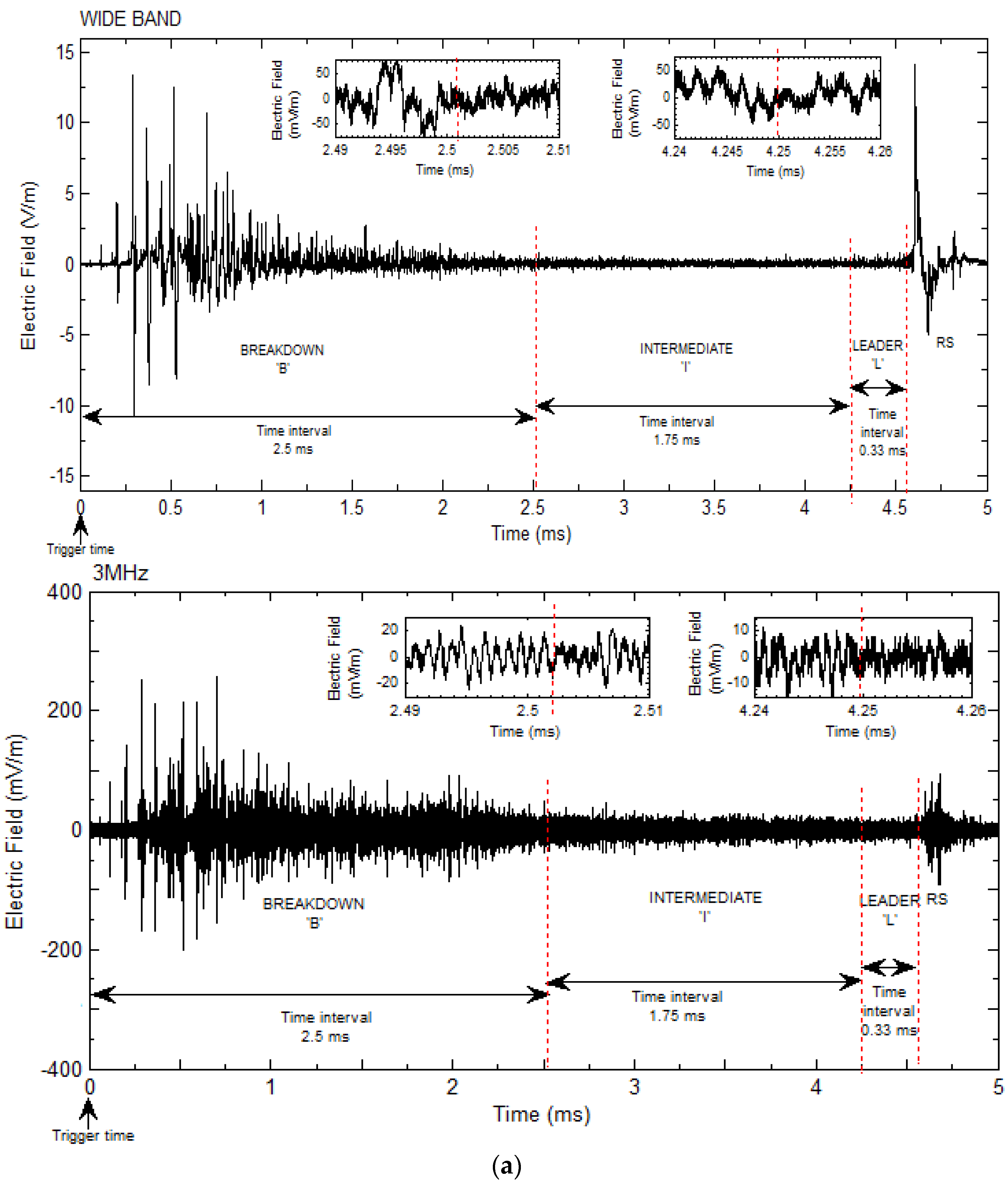
Figure 1.
Simultaneous electric field records of negative cloud-to-ground lightning flash at wide bands and at 3 MHz. (
a) A typical example of “B” “I” “L” type flash that was recorded on 19/07/2014 at 16:05:22:005374. Total time frame of the record was 250 ms but only 5 ms from the trigger time is shown and the distance to the strike location (60.08570°N, 17.27850°E) was 30 km from the measuring station. Note that the pulses around the transition from “B” to “I” and from “I” to “L” are shown in a smaller time window of 0.02 ms. (
b) An example of “B” “L” type structure recorded on 19/07/2014 at 15:48:45:303558. The record length was 250 ms but only 3 ms from the trigger time is shown and the strike location (60.22760°N, 17.48430°E) was 34.39 km away. In the inset, the transition between “B” and “L” are shown. (
c) Pulse structure around the transition from “B” to “L” in the case of “B” “L” type structure (shown in
Figure 1b) is shown in a 0.05 ms time window.
Table 2 contains a statistical presentation of the temporal features of PB pulses based on this study. For comparison, data from Nag and Rakov [
4] and Baharudin
et al. [
8] is also added. From the present study in Sweden, the average individual pulse duration of the PB pulses, pertinent to the temperate region (humid continental), is found to be 19 µs, which is slightly higher than that at the humid subtropical region (Florida) (17 µs), and significantly higher than that observed in the wet tropics (Malaysia) (11 µs).
Table 2.
Statistical presentation of the temporal features of preliminary breakdown (PB) pulses.
Table 2.
Statistical presentation of the temporal features of preliminary breakdown (PB) pulses.
| Study | No. of Samples | Parameter |
|---|
| Individual Pulse Duration | Inter-Pulse Interval | Total of Pulse Train |
|---|
| Arithmetic Mean (µs) | Range (µs) | Arithmetic Mean (µs) | Range (µs) | Arithmetic Mean (ms) | Geometric Mean (ms) | Range (ms) |
|---|
| Present study Sweden | 33 | 18.63 | 2.2–47.49 | 53.63 | 7.49–185.46 | 2.60 | 2.49 | 1.39–6.15 |
| Nag and Rakov [4] (2008a) Florida | 35 | 17 | 1–91 | 73 | 1–530 | 2.70 | 2.3 | 0.8–7.9 |
| Baharudin et al. [8] (2012) Malaysia | 24 | 11 | 1–92 | 152 | 1–1908 | 12.30 | 10.1 | 2–37 |
Further, the PB inter-pulse interval in the temperate region (Sweden) is slightly lower (54 µs) than that in the sub tropics (73 µs) and lowest as compared to the tropics (152 µs). From the range of inter-pulse interval given for three different latitudes, there seems to be a significant difference between the temperate region (Sweden) and the wet tropics (Malaysia). The difference in the inter-pulse interval can be viewed as the function of latitude, however, more data from other geographical locations is needed for any conclusion.
In addition, we can see from
Table 2, the total duration of the PB pulse train pertinent to the temperate region (this study, 2.6 ms, Sweden) is comparable to that of subtropics (Nag and Rakov [
4], 2.7 ms, Florida) but significantly shorter than that of the tropics (Baharudin
et al. [
8], 12.30 ms, Malaysia).
Comparing the duration from three geographical locations, it can be said that the total duration of pulse train decreases with the increase in latitude, Malaysia (tropics) having the maximum and Sweden (the highest latitude) having minimum. Such a variation in the pulse train can be attributed to the difference in metrological conditions, region, altitude of cloud and temperature.
3.1.2. PB to RS Ratio
To have an idea about the comparative electric field strength of PB pulses and the following RS, the amplitude ratio of the electric fields of the highest PB pulse to that of the following RS has been analyzed. This is similar to the previous works by several authors e.g., Gomes
et al. [
3], Mäkelä
et al. [
6], Nag and Rakov [
7], Baharudin
et al. [
8], Cooray and Jayaratne [
17] and Gomes and Cooray [
18]. However, in the present study, electric field strengths from the PBP and the following RS at 3 and 30 MHz have also been taken into account.
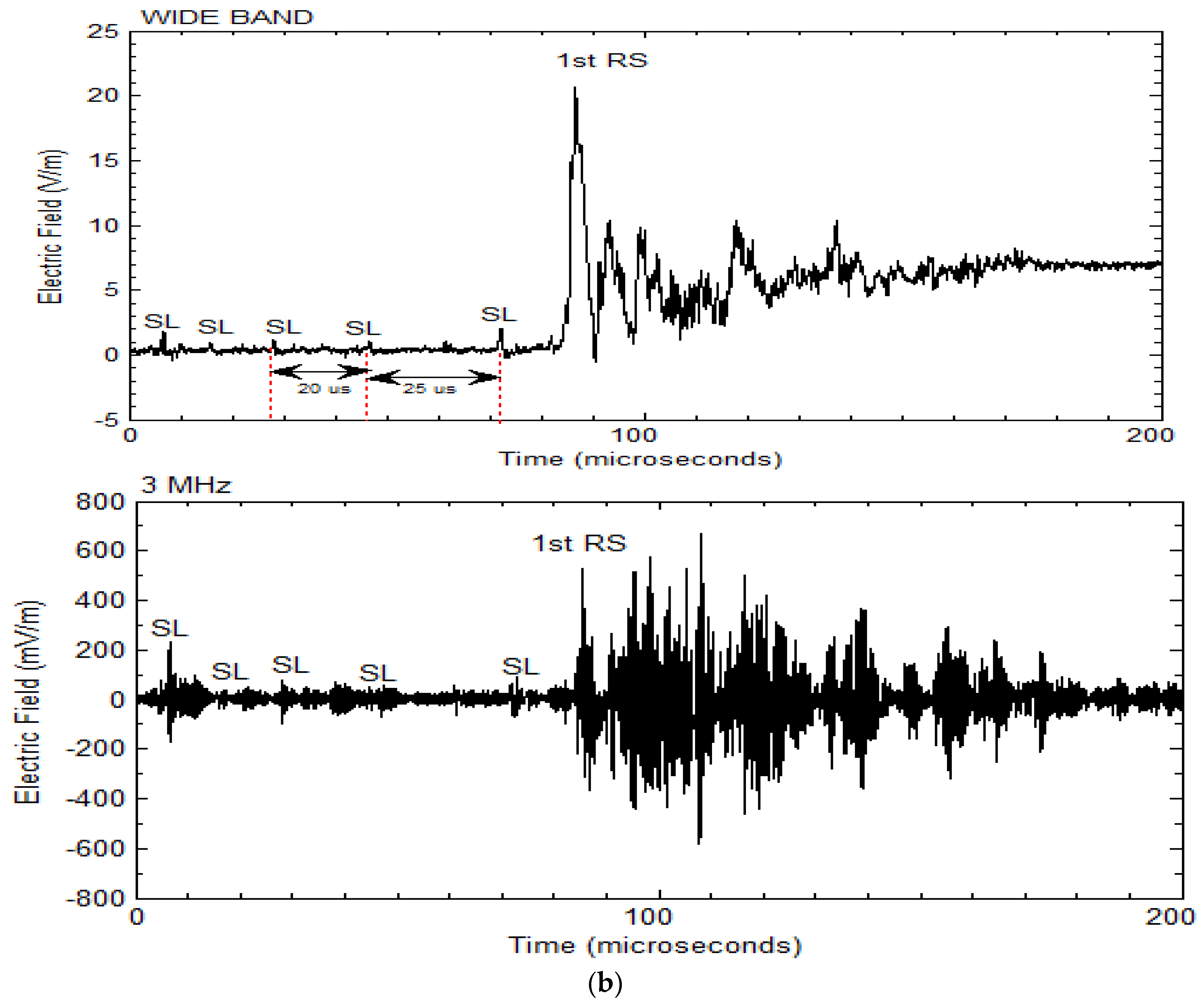
Figure 2 depicts three PB pulse trains at wideband, 3 and 30 MHz with pulse polarities identical to each other.
Figure 3 shows an example where the amplitude of the preliminary breakdown pulse exceeds that of the return stroke. In addition, the preliminary breakdown pulse activity above the noise can be clearly observed.
The distribution of PB to RS ratio of flashes observed in Sweden is given in
Table 3. The arithmetic mean, the geometric mean, and the standard deviation of the PB to RS ratio at wideband are obtained to be about 0.7, 0.5 and 0.8, respectively. The minimum and the maximum values of the ratios observed are 0.03 and 6, respectively. As it was mentioned earlier, this analysis also introduces PB to RS ratio at narrowband frequency. From 98 flashes, the arithmetic mean, geometric mean and standard deviation of PB/RS ratio at 3 MHz are found to be about 1.9, 1.6 and 1.5, respectively, with a maximum and minimum value of 0.06 and 11, respectively. Meanwhile, from eight flashes, arithmetic mean, geometric mean and standard deviation for the electric field at 30 MHz are 1.4, 1.3 and 0.65, respectively, with a range from 0.56 to 2.4.
Figure 2.
Wideband PB pulse train together with 3 and 30 MHz recorded in 21/07/2014 at 16:48:02:497955 for negative cloud-to-ground flash. The strike location (59.79490°N, 17.64630°E) was located at a distance of about 7 km from the measuring station. (a) Record of the whole flash; (b) Portion of the PB pulse train with maximum amplitude (zoomed from 2a). Note that the zoomed pulse starts at the trigger time, zero and ends 40 μs after.
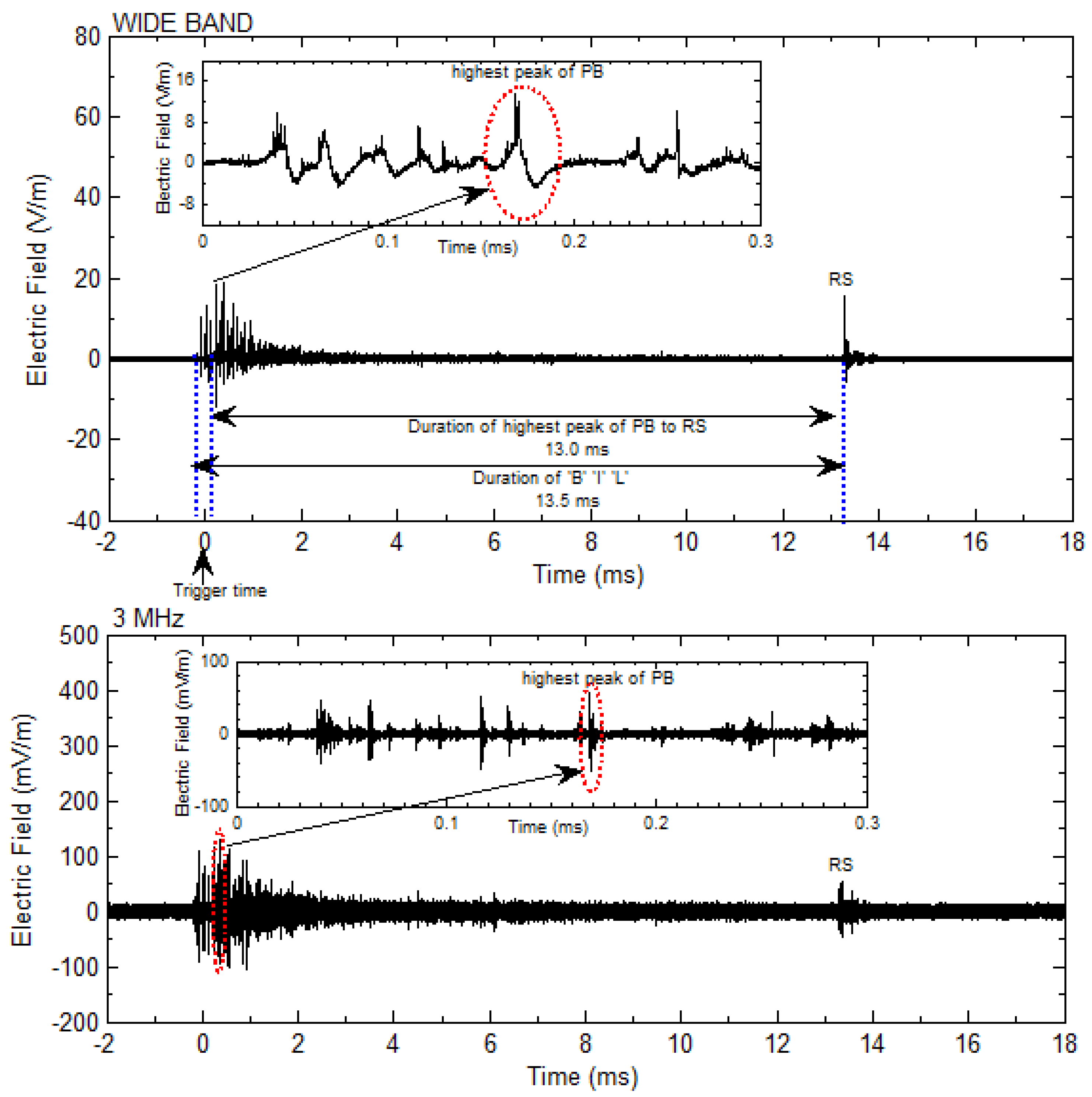
Figure 3.
A sample of flashes with higher PB amplitudes compared to the following RS recorded on 19/07/2014 at 15:58:26:656472 located at a distance of 34.89 km from the measuring station where the strike location was at (60.10540°N, 17.32080°E). (top figure) A wideband record of the flash showing the PB together with the first RS. (bottom figure) the 3 MHz record of the same flash as in the top figure. Note that the highest peak of the PB pulse trains of wideband and 3 MHz signals is shown in the inset of the respective figures.
Table 3.
Preliminary breakdown (PB) to return stroke (RS) electric field peak ratio.
Table 3.
Preliminary breakdown (PB) to return stroke (RS) electric field peak ratio.
| Location | No of Flash | PB/RS Ratio (Electric Field Amplitude) | Noise/RS Ratio |
|---|
| Arith. Mean | Geometric Mean | Minimum | Maximum | Std Deviation | Median | Arithmetic Mean | Geometric Mean |
|---|
| Present study Sweden wideband | 98 | 0.706 | 0.467 | 0.032 | 5.996 | 0.775 | 0.472 | 0.021 | 0.013 |
| Present study Sweden 3 MHz | 98 | 1.92 | 1.56 | 0.63 | 11.19 | 1.46 | 1.50 | 0.19 | 0.13 |
| Present study Sweden 30 MHz | 8 | 1.39 | 1.26 | 0.56 | 2.44 | 0.65 | 1.30 | 0.36 | 0.35 |
| Baharudin et al. [8] Malaysia (2012) | 97 | 0.278 | 0.146 | 0.026 | 2.281 | 0.422 | 0.122 | 0.07 | 0.06 |
| Nag & Rakov [7] Florida 27°N (August 2009a) | 100 | 0.294 | 0.223 | 0.029 | 1.49 | 0.236 | 0.215 | 0.023 | 0.02 |
| Nag and Rakov [7] Florida 30°N (April 2009a) | 59 | 0.62 | 0.45 | 0.16 | 5.10 | - | - | - | - |
| Mäkelä et al. [6] Finland (2008) | 193 | 0.61 | 0.25 | 1.0 | 6.10 | - | - | - | - |
| Gomes et al. [3] Sweden (1998) | 41 | 1.01 | 0.485 | 0.083 | 6.27 | - | - | - | - |
| Gomes et al. [3] Sri Lanka (1998) | 9 | 0.165 | 0.146 | 0.062 | 0.264 | - | - | - | - |
The arithmetic mean and geometric mean of the noise peak to the return stroke ratio (N/RS) are found to be about 0.02 and 0.01, respectively. Observe that the minimum PB to RS ratio measured in the present study is greater than the mean of noise to RS by an approximate factor of 1.5 (0.03/0.02). From this observation, we can conclude that the ambient noise has not affected the results significantly. The same trend can be seen even for 3 MHz and 30 MHz signals.
We summarized and compared the results obtained earlier by [
3,
6,
7,
8] to the results obtained in the present study as shown in
Table 3. Note that the means of the PB to RS ratio are relatively high in temperate regions such as in Sweden and Finland compared to tropical regions such as Malaysia and Sri Lanka. It seems that there are more PB activities at higher latitudes whereas we can see a mixed results from a mid-latitude region like Florida [
7]. Data from tropical regions regarding 3 MHz and 30 MHz signals are not available in the literature but, as can be seen, the PB to RS ratio for 3 MHz and 30 MHz signals is higher than the wideband signals in Sweden indicating that the PB pulses are the strong radiator of 3 and 30 MHz electric field radiations. This is in agreement with the argument by [
17,
19] that, at higher latitudes the detection of stronger PB pulse train in the flash, could be due to the stronger lower positive charge region (LPCR) below the main negative charge centre. The height of the cloud from the ground can also be attributed for the detection of 3 and 30 MHz electric fields in the higher latitudes. Both, stronger LPCR and lower cloud height can lead to the higher probability of ground flashes.
3.2. Stepped Leader (SL)
3.2.1. The Beginning of the Stepped Leader
The inception of PB activity in the cloud may lead to stepped leaders that, in turn, can lead to return strokes. The stepped leader may immediately succeed the PB pulse train without any pause or may succeed the PB with a pause in between. The pause, is being referred to as intermediate stage in the BIL structure even though some researcher [
20] interpreted the BIL structure as the start and the continuation of the stepped leader without having any “pause”. Researchers such as Gomes
et al. [
3], Beasley
et al. [
21] and Thomson [
22] have used different techniques to identify the beginning of the stepped leader field. However, according to Cooray [
23], a major problem in evaluating the duration of stepped leader field is caused by difficulty to pinpoint its exact beginning. In the present analysis, we observed that the 3 MHz signal follows the wideband signal so that the start of the stepped leader is clear after the intermediate stage in the case of BIL structure. It is shown in
Figure 1a. In the inset of the 3 MHz signal, one can see how the oscillations have become more intensive after the intermediate stage and we can see, at the corresponding time in the inset of the wideband signal, there is a transition. We also observed that in the case of BL structure the 3 MHz signal shows a “transition phase” with no significant variations in amplitudes between the “B” and “L” phase. This is shown in
Figure 1b,c. The corresponding part on the wideband signal shows slow field changes between the “B” and “L” as shown in
Figure 1c. To identify the beginning of the stepped leader in the case of BL structure, this comparison between the wideband and the 3 MHz signals was used. We can consider the start of a leader when 3 MHz signal showed a “transition phase” with no significant amplitude variations after breakdown (“B”) region in the corresponding wideband signal. The physical process that signifies this transition is not understood yet. However, as this appears consistently and repeatedly, we utilized this piece of information to indicate the beginning of the stepped leader. It will be interesting to follow-up on this.
3.2.2. SL to RS Ratio
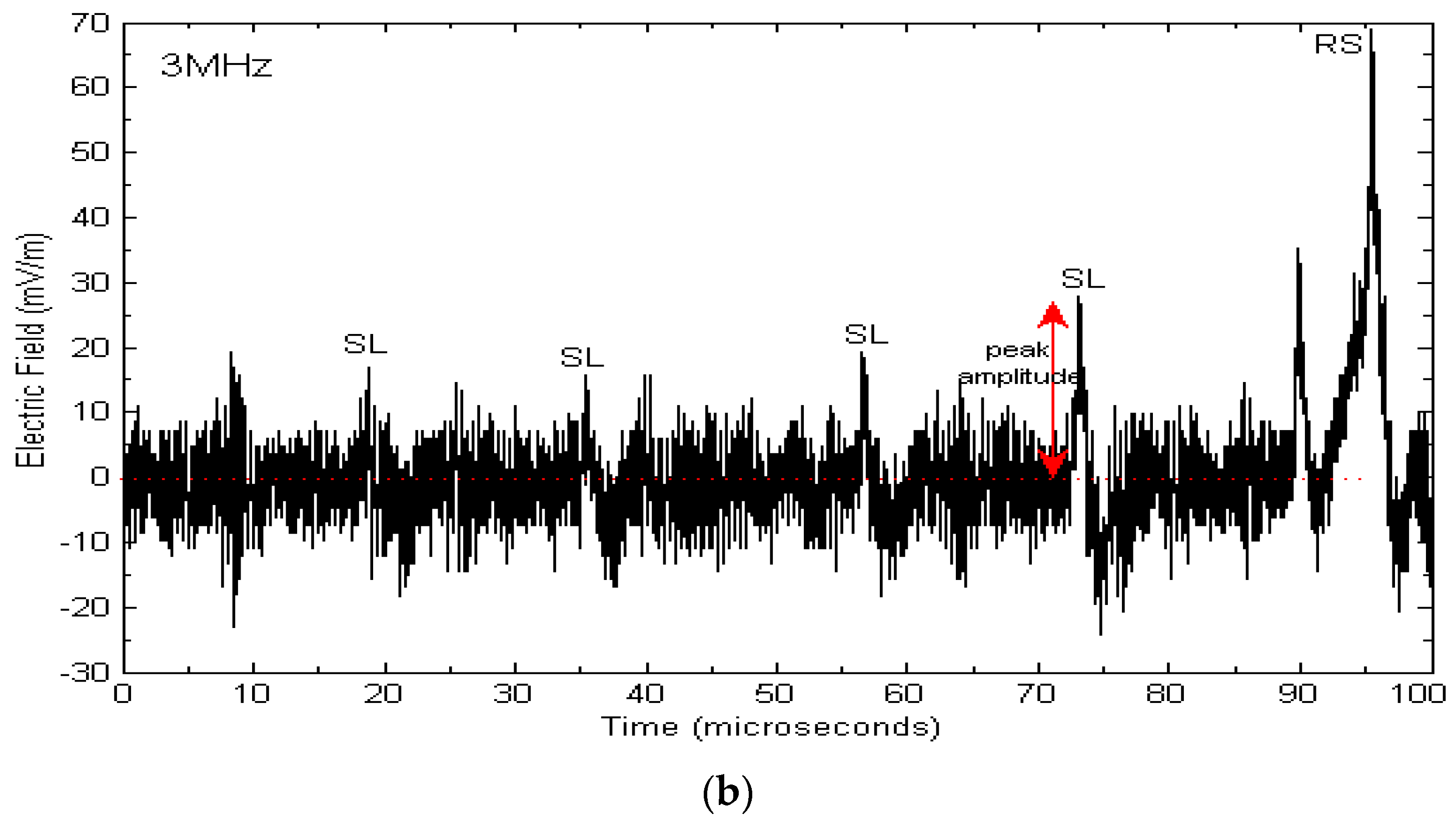
For the purpose of comparison of the amplitudes of the electric fields by the stepped leaders and the following return strokes, the last pulse of the “B” “I” “L” or “B” “L” was considered as the stepped leader amplitude as shown in
Figure 4. From
Table 4, it can be seen that the arithmetic and geometric means of SL/RS is 0.14 and 0.11, respectively, for the wideband signals. However, for 3 MHz signals, the ratio (SL/RS) is much larger (the arithmetic and the geometric mean is 0.42 and 0.38 respectively) than that of the wideband signals. For the comparison of SL/RS ratio at 3 MHz only 86 flashes out of 98 were selected, because amplitudes of the stepped leaders for only 86 flashes were higher than that of noise and the remaining 12 flashes had the amplitudes similar to the amplitudes of the noise.
The stepped leaders preceding the return stroke generates weaker electric fields as compared to the following return strokes. The magnitude of step current can be attributed for the weaker field.
Table 4.
Stepped leader (SL) to RS electric field amplitude ratio.
Table 4.
Stepped leader (SL) to RS electric field amplitude ratio.
| Location | No of Flash | SL/RS Ratio (Electric Field Amplitude) | Noise/RS Ratio |
|---|
| Arithmetic Mean | Geometric Mean | Minimum | Maximum | Std. Deviation | Median | Arithmetic Mean | Geometric Mean |
|---|
| Present study Sweden Wideband | 98 | 0.14 | 0.11 | 0.03 | 0.75 | 0.13 | 0.10 | 0.02 | 0.01 |
This study Sweden
3 MHZ | 86 | 0.42 | 0.38 | 0.11 | 1.14 | 0.19 | 0.39 | 0.19 | 0.13 |
Figure 4.
A section of the flash in which stepped leaders at (a) wideband and (b) 3 MHz are shown. Recorded on 19/07/2014 at 18:25:47:489,798 from a flash located (60.18510°N, 17.87690°E) at a distance of 40.76 km from the measuring station T = 0 was 7.6630 ms from the trigger time.
Figure 4.
A section of the flash in which stepped leaders at (a) wideband and (b) 3 MHz are shown. Recorded on 19/07/2014 at 18:25:47:489,798 from a flash located (60.18510°N, 17.87690°E) at a distance of 40.76 km from the measuring station T = 0 was 7.6630 ms from the trigger time.
3.3. Subsequent Return Stroke (SRS)
3.3.1. Inter-Stroke Interval
Once the attachment is established between the cloud and the ground through the stepped leader followed by the return stroke, a rapid neutralization takes place that may involve continuing current and some cloud activity. However, more often, the residual first-stroke channel is traversed downwards by a dart or dart-stepped leader. When a dart or dart-stepped leader approaches the ground, another attachment and neutralization process called subsequent return stroke takes place. A lightning ground flash may involve several of these subsequent return strokes. In order to determine that the strokes belong to the same flash, we consider the time separation between strokes and, if this time is shorter than about 500 ms, we consider the strokes from the same flash [
24]. However, of course, as the total time window was 250 ms in this study, effectively this time separation set the limit. Depending on the path that subsequent return strokes take, there could be two different types of strokes with different properties. We did not have any means to determine whether a subsequent return stroke followed the existing ionized channel or it created a new channel in virgin air. In this study, we have analyzed the inter-stroke interval which is the duration between two consecutive return strokes. As it is seen from the
Table 5, the arithmetic and geometric means of inter-stroke interval were 40 ms and 37 ms respectively with a range of 2 ms to 142 ms, based on 98 flashes and a total of 206 subsequent return strokes. This value of inter-stroke interval is apparently the minimum among all the measurements carried out at different geographical locations as is seen from the
Table 5. One of the reasons for this could be the record length in the present study which was set to 250 ms, whereas other researchers have used the record length of 1 s and above. It is evident from the
Table 5 that there is a tendency for the inter-stroke interval to be dependent on geographical regions. The arithmetic mean values of the inter-stroke interval for tropical regions (Sri Lanka [
1], Malaysia [
9], Papua New Guinea [
22] and Brazil [
25]) lie between 83 and 90, whereas it lies between 64 and 65 for temperate regions (Sweden [
2] and China [
26]).
Table 5.
Inter-stroke interval for Subsequent Return Strokes (SRS).
Table 5.
Inter-stroke interval for Subsequent Return Strokes (SRS).
| Researcher and Location | Total Flashes | Total Subsequent Return Strokes | Minimum (ms) | Maximum (ms) | Arithmetic Mean (ms) | Geometric Mean (ms) | Record Length (s) |
|---|
| Present study Sweden, six summer thunderstorm | 98 | 206 | 2.15 | 142.46 | 40.78 | 37.74 | 0.25 |
| Baharudin et al. [9] Malaysia, (2014) seven convective thunderstorm | 100 | 305 | 0.5 | 461 | 86 | 67 | 1 |
| Saba et al. [25] Brazil, (2006) twenty-seven frontal and convective thunderstorm | 186 | 608 | 2 | 782 | 83 | 61 | 1 |
| Qje et al. [26] China, (2002) nine Summer thunderstorm | 50 | 238 | 4.8 | 328.5 | 64.3 | 46.6 | 1 |
| Cooray and Jayaratne [1] Sri Lanka, (1994) three convective thunderstorm | 81 | 284 | 0.98 | 509 | 82.8 | 56.5 | 1 |
| Cooray and Perez [2] Sweden, (1994) two frontal summer thunderstorm | 271 | 568 | 2.5 | 376 | 65 | 48 | 1 |
| Thottappillil et al. [27] Florida (1992) three convective summer thunderstorm | 46 | 199 | - | - | - | 57 | 1 |
| Thompson [22] Papua New Guinea, (1980) Convective Orographic | 80 | 202 | - | - | 90 | 61 | 1 |
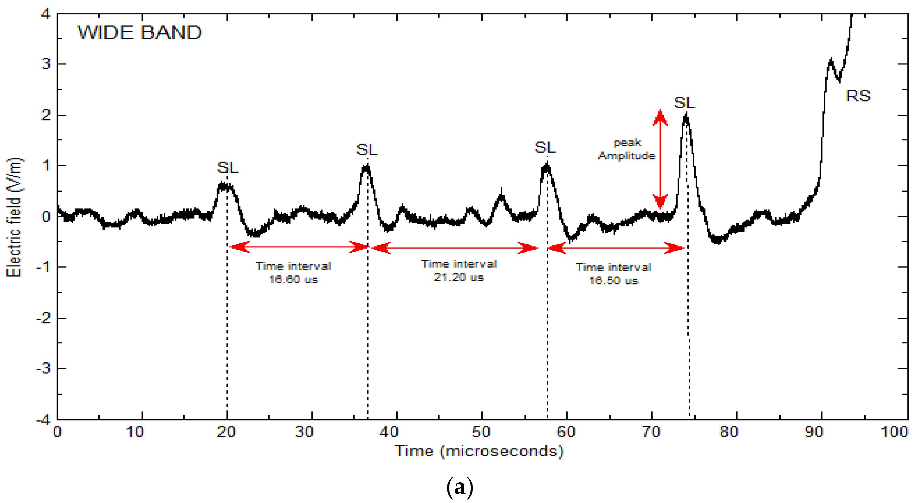
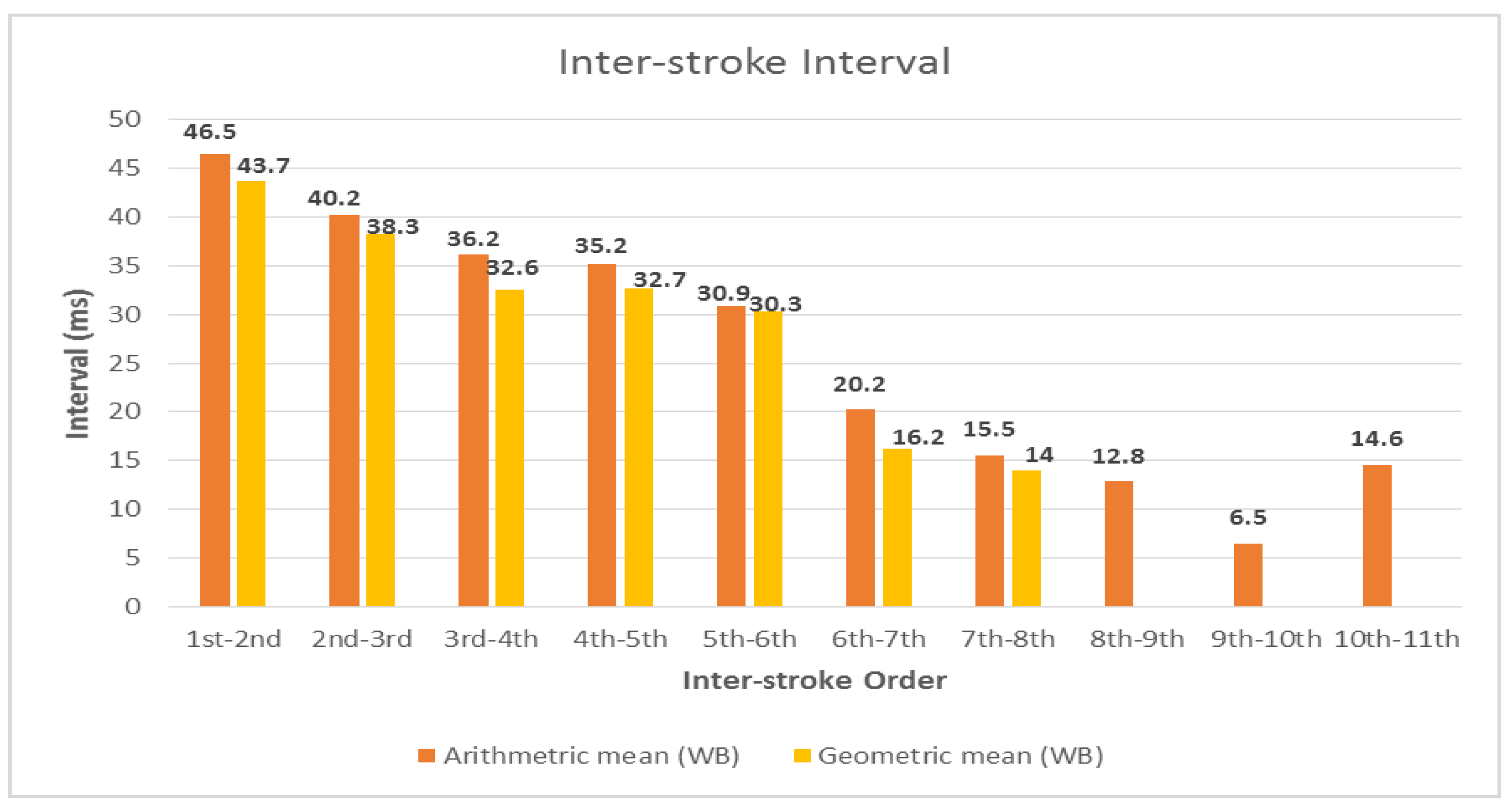
Figure 5 shows the trend of inter-stroke interval between the successive return strokes in order, and it is seen that the interval seems to decrease with certain variation. The interval between the first RS and the first SRS show high arithmetic and geometric means than other intervals which is 46 ms and 43 ms, respectively.
Figure 5.
Inter stroke interval of SRS order, WB = wideband.
Figure 5.
Inter stroke interval of SRS order, WB = wideband.
3.3.2. The Average Peak Value of SRS to RS Peak Ratio
The strength of the electric field produced by the return strokes is related to the value of the current in the channel and its derivative. A comparative analysis of the electric fields produced by the first RS and the SRS would imply the comparative magnitudes of peak currents. As mentioned earlier, this study is based on a total of 98 flashes which contained a total of 206 SRS. In this section, we present the ratio of SRS (the average of all SRS values) to the corresponding first RS electric field peaks and the result is presented and compared with other studies as can be seen in
Table 6. As it is seen from the
Table 6, the ratio (at wideband, this study) ranges from 0.12 to 2.52 with the arithmetic and geometric means 0.46 and 0.35, respectively. Considering the strength of the subsequent return strokes as compared to the first return strokes, the average ratio of electric field strength at wideband of the subsequent return strokes to the corresponding return stroke is found to be 0.46. This implies that the electric field produced by the subsequent return stroke is weaker than that by the first return stroke. This is expected as the subsequent return strokes transport the charge through a relatively conductive path and with less branching. Whereas, at 3 MHz, the arithmetic mean is 1.05 and the geometric mean is 0.77. This shows that on average all SRS radiate electric fields at 3 MHz almost with the same amplitudes as the first RS.
Table 6.
Subsequent return strokes (SRS) to RS ratio.
Table 6.
Subsequent return strokes (SRS) to RS ratio.
| Researcher and Location | Total of Subsequent Strokes | Minimum | Maximum | Arithmetic Mean | Geometric Mean | Standard Deviation | Median |
|---|
| Present study Sweden (Wide band) | 206 | 0.12 | 2.52 | 0.46 | 0.35 | 0.38 | 0.32 |
| Present study Sweden (3 MHz) | 206 | 0.08 | 9.69 | 1.05 | 0.77 | 0.93 | 0.86 |
| Baharudin et al. [9] Malaysia (2014) | 301 | 0.13 | 2.80 | 0.73 | 0.60 | 0.48 | 0.67 |
| Nag et al. [5] Florida (2008b) | 239 | 0.13 | 8.3 | 0.75 | 0.58 | - | - |
| Schulz et al. [28] Sweden (2008) | 258 | 0.08 | 3.3 | 0.64 | 0.52 | - | - |
| Oliveira Filho [29] Brazil (2007) | 909 | 0.08 | 4.3 | 0.69 | 0.53 | - | - |
| Schulz and Diendorfer [30] Austria (2006) | 247 | 0.04 | 3.7 | 0.87 | 0.64 | - | - |
| Qie et al. [26] China (2002) | 238 | 0.04 | 3.8 | 0.70 | 0.46 | - | - |
| Cooray and Jayaratne [1] Sri Lanka (1994) | 284 | 0.03 | 2.3 | 0.55 | 0.44 | - | - |
| Cooray and Perez [2] Sweden (1994) | 314 | 0.09 | 2.4 | 0.63 | 0.51 | - | - |
| Thottapillil et al. [27] Florida (1992) | 199 | - | - | - | 0.42 | - | - |
For the sake of comparison, results from different geographical locations along with the present study has been depicted in
Table 6. The geometric mean of the SRS to RS ratio observed in Sweden (present study) is compared to those measured in Sri Lanka [
1], Sweden [
2], Florida [
5], Malaysia [
9], China [
26], Florida [
27], Sweden [
28], Brazil [
29] and Austria [
30]. One can notice that the SRS/RS ratio does not show any latitude dependency.
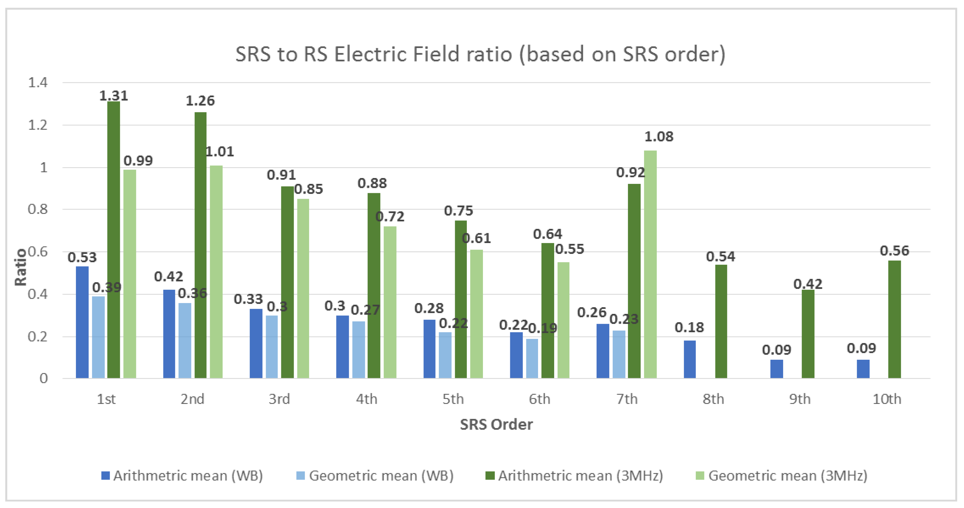
Figure 6 shows the trend SRS to RS ratio at the successive return strokes in order, and it is seen that the ratio decreases in general with some variation from first RS to last successive SRS. The electric field ratio SRS to RS at first SRS show high arithmetic and geometric mean than others which is 0.53 and 0.39 respectively for wideband and 1.31 and 0.99, respectively, for 3 MHz radiation.
Figure 6.
The SRS to RS electric field amplitude ratio based on SRS order with 3 MHz. WB = wideband.
Figure 6.
The SRS to RS electric field amplitude ratio based on SRS order with 3 MHz. WB = wideband.
3.3.3. Individual Peaks of SRS to First RS Peak Ratio
In the present study, the individual SRS peak values were also analyzed and compared with those of the first RS in order to understand the possible differences involved in the physical processes between these phenomena.
Figure 7a–d depict the examples of SRS peak larger than the first RS. Shown in
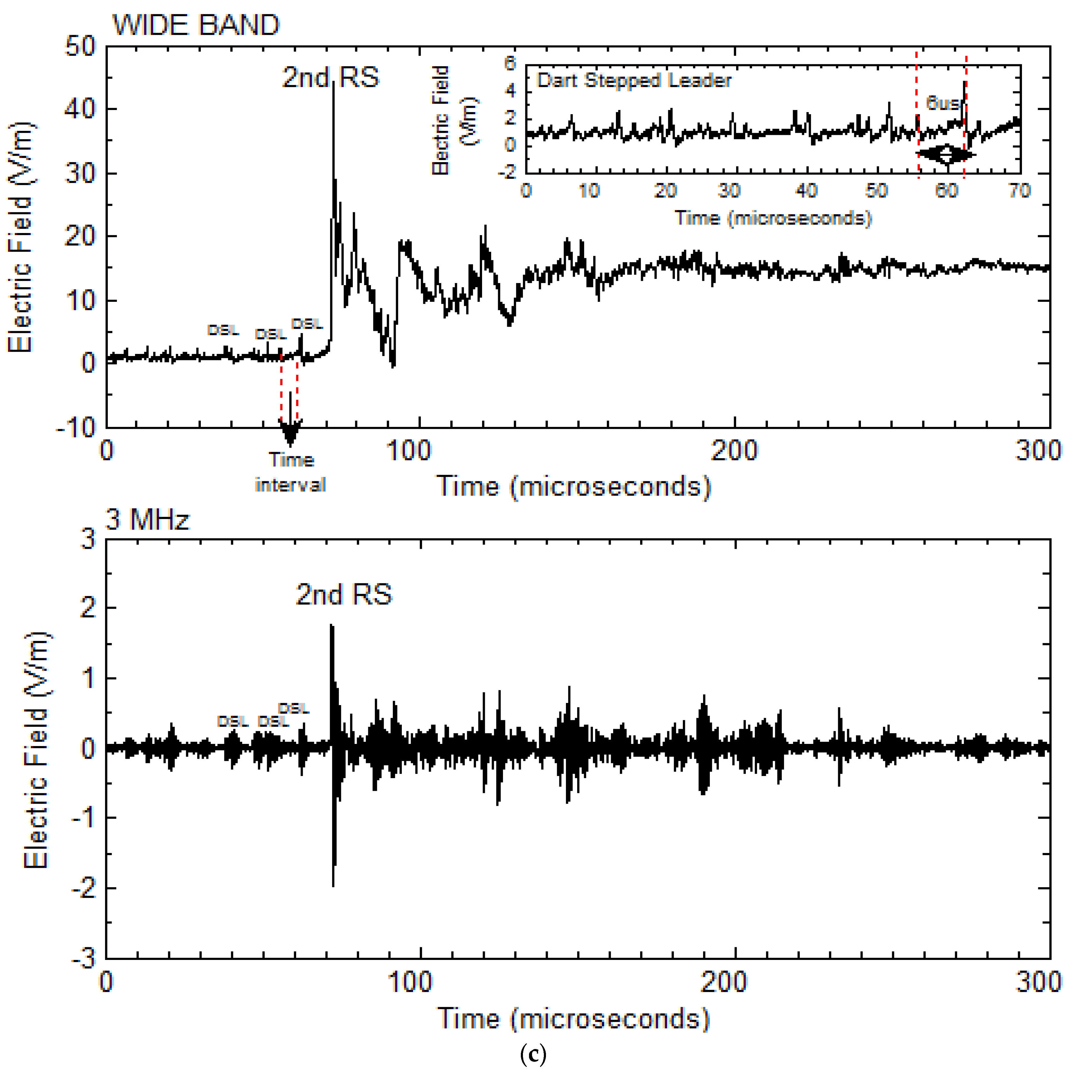
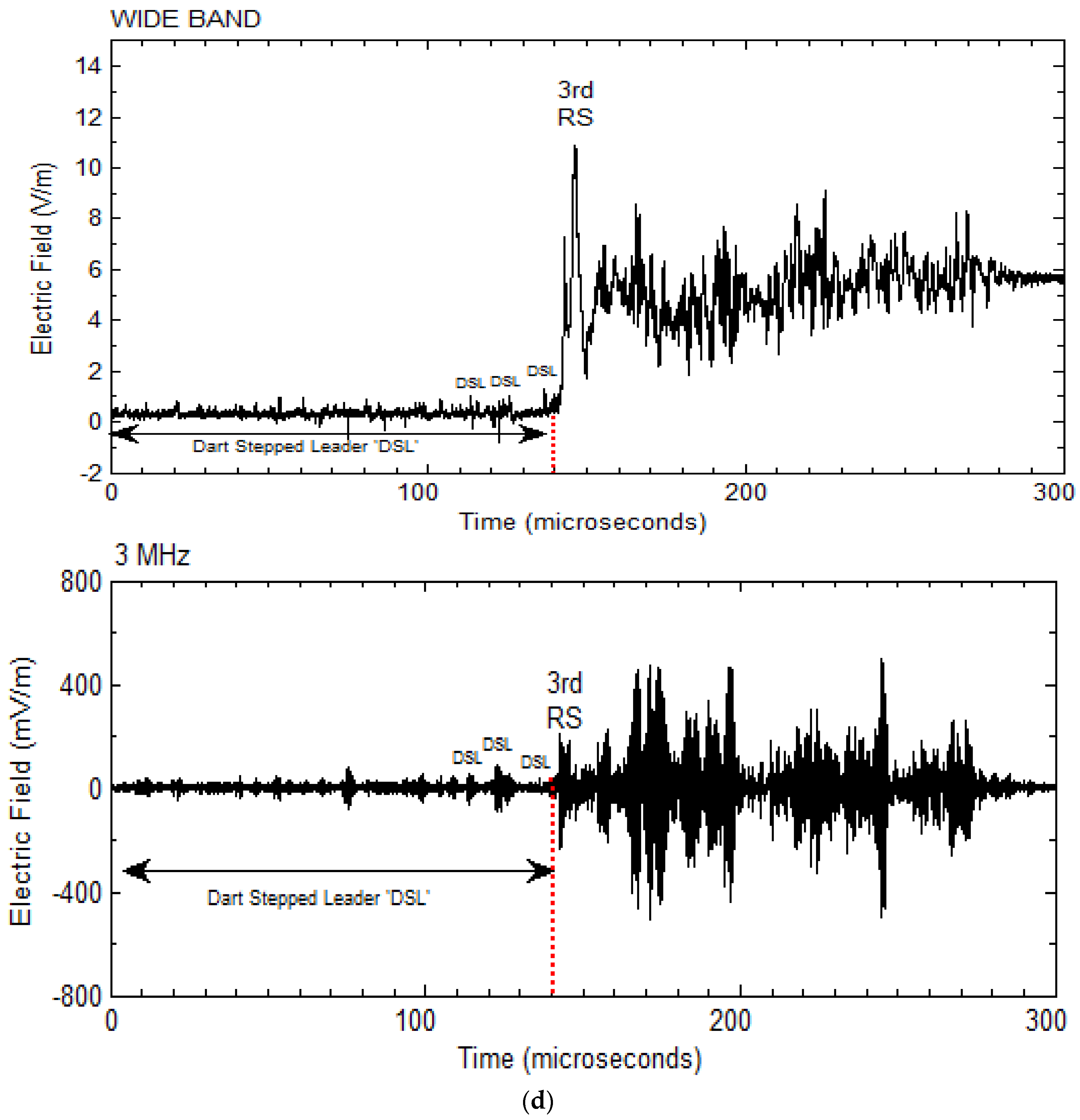
Figure 7a is an example of a negative CG flash in which the first SRS is stronger than the first RS.
Figure 7b–d shows all three strokes from
Figure 7a on a smaller time scale where on slow field changes stepped and dart-stepped leaders are also marked. In order to determine the type of pulses, we use the following conditions. When the time separation between two consecutive pulses is larger than 10 μs, we consider those pulses as stepped leader pulses whereas when the time separation is shorter than 10 μs, we consider those as dart-stepped leaders. Because, according to Krider
et al. [
31], the average time interval between the pulses of the radiation field produced by the dart-stepped leaders is about 6–8 μs. This was confirmed by Orville and Idone [
32] where the average was 5–10 μs, which is shorter than about 10–15 μs observed for the stepped leaders. This is also justified by our data that shows the maximum time separation between all identified dart-stepped leaders was 9.4 μs. The ratio of amplitude of electric fields produced by the first and the individual subsequent return strokes were compared as it is shown in
Table 7. It seems that at 3 MHz the individual peaks of SRS to RS peak ratio is decreasing for the every following SRS. The first SRS produces the strongest electric field at wideband as well as at 3 MHz followed by the second, third and fourth SRS. Note that 19 strokes out of 206 subsequent strokes had electric field peaks larger than the first RS as can be found in
Table 8.
Table 7.
Statistics of SRS having higher peak values than the first RS, distance to strike location is shown.
Table 7.
Statistics of SRS having higher peak values than the first RS, distance to strike location is shown.
| Type of Duration | Distance Range (km) | Total of Stroke | Arithmetic Mean (µs) | Geometric Mean (µs) | Maximum (µs) | Minimum (µs) | Standard Deviation (µs) | SRS to 1st RS Peak Ratio (Wide Band) | SRS to 1st RS Peak Ratio (3 MHz) |
|---|
| 1st RS | 6–32 | 16 | | | | | | - | - |
| Pulse width | 21.22 | 20.39 | 35.2 | 12.1 | 6.15 |
| Slow front | 2.86 | 2.37 | 7 | 0.79 | 1.80 |
| Rise Time | 3.36 | 2.97 | 5.7 | 1.05 | 1.54 |
| 2nd RS | 6–31 | 13 | | | | | | A.Mean | A.Mean |
| Pulse width | 17.93 | 17.45 | 24.8 | 10.62 | 4.25 | 1.65 | 2.61 |
| Slow front | 1.30 | 1.16 | 2.75 | 0.6 | 0.69 | G.Mean | G.Mean |
| Rise Time | 1.92 | 1.46 | 4.15 | 0.75 | 1.22 | 1.52 | 2.07 |
| 3rd RS | 8–32 | 3 | | | | | | A.Mean | A.Mean |
| Pulse width | 17.69 | 17.66 | 18.96 | 16.567 | 1.20 | 1.24 | 2.07 |
| Slow front | 1.54 | 1.50 | 1.95 | 1.08 | 0.44 | G.Mean | G.Mean |
| Rise Time | 2.61 | 2.40 | 4.15 | 1.58 | 1.36 | 1.21 | 1.71 |
| 4th RS | 10–17 | 3 | | | | | | A.Mean | A.Mean |
| Pulse width | 16.34 | 16.31 | 17.65 | 15.15 | 1.25 | 1.25 | 1.71 |
| Slow front | 2.083 | 2.082 | 2.14 | 1.98 | 0.08 | G.Mean | G.Mean |
| Rise Time | 2.81 | 2.42 | 3.2 | 1.67 | 0.78 | 1.24 | 1.50 |
Table 8.
Percentage of flashes with higher SRS peaks and percentage of SRS with higher peaks than the first RS.
Table 8.
Percentage of flashes with higher SRS peaks and percentage of SRS with higher peaks than the first RS.
| Researcher and Location | Total Number of Flashes | Number of Flashes with at Least one SRS Field Larger than the First RS | Percentage of Flashes with at Least one SRS Field Larger than the First RS, % | Total Number of SRS | Number of SRS with Field Peaks Larger than the First RS | Percentage of SRS with Field Peaks Larger than the First RS, % |
|---|
| Present study Sweden (Wide band) | 98 | 16 | 16.47 | 206 | 19 | 9.22 |
| Present Study Sweden (3 MHz) | 98 | 58 | 58.82 | 206 | 95 | 46.12 |
| Baharudin et al. [9] Malaysia (2014) | 100 | 38 | 38 | 301 | 57 | 19 |
| Nag et al. [5] Florida (2008b) | 176 | 42 | 24 | 239 | 50 | 21 |
| Schulz et al. [28] Sweden (2008) | 93 | 30 | 32 | 258 | 46 | 18 |
| Oliveira Filho et al. [29] Brazil (2007) | 259 | 98 | 38 | 909 | 182 | 20 |
| Schulz and Diendorfer [30] Austria (2006) | 81 | 40 | 49 | 247 | 79 | 32 |
| Qie et al. [26] China (2002) | 50 | 27 | 54 | 238 | 53.8 | 22.6 |
| Cooray and Jayaratne [1] Sri Lanka (1994) | 81 | 28 | 35 | 284 | 35 | 12.3 |
| Cooray and Perez [2] Sweden (1994) | 276 | 66 | 24 | 479 | 72 | 15 |
| Thottapillil et al. [27] Florida (1992) | 46 | 15 | 33 | 199 | 26 | 13 |
It can also be seen from
Table 7 that the duration of SRS pulses are relatively narrower than the first RS. The individual pulsewidth of the first return stroke is about 21 µs whereas that of first, second and third subsequent return strokes are about 18 µs, 18 µs and 16 µs respectively. Further, the first subsequent return stroke has apparently fast rise time and shorter slow front compared to the first return stroke and other subsequent return strokes as shown in the
Table 7. This is indicative of the fast charge transfer during the subsequent return stroke as compared to the first return stroke.
The percentage of multiple stroke flashes having at least one SRS with a peak electric field larger than the first RS in Sweden (2014) was about 16%.
Table 8 shows the percentage of flashes having at least one SRS with a peak electric field being larger than the first RS in Sri Lanka [
1], Sweden [
2], Florida [
5], Malaysia [
9], China [
26], Florida [
27], Sweden [
28], Brazil [
29] and Austria [
30] are 35%, 24%, 24%, 38%, 54%, 33%, 32%, 38% and 49%, respectively. These differences can partly explained due to different time windows and partly due to different meteorological parameters.
Figure 7.
(
a) A sample of SRS peak larger than first RS, recorded on 21/7/2014 at 16:56:12:679,187. The distance from the measuring station to the first stroke location (59.80380°N, 17,74230°E) was about 8 km. (
b,
c,
d) shows three return strokes from
Figure 7a on smaller time scales respectively. Note that the slow field changes are also visible and stepped leader (SL) and dart-stepped leader (DSL) are marked. (
e) Maximum stroke multiplicity in Sweden 2014 measurement campaign together with 3 MHz, recorded on 21/07/2014 at 15:34:54:829297. The distance from the measuring station to the first stroke location (59.7350°N, 17.5280°E) was 13.5 km.
3.4. Some Aspects of the Complete Flash
Here, we report some other aspects observed from the complete recorded flashes pertinent to the negative CG flashes in Sweden. Whenever there are some fine structures in the wideband signal, we notice that the 3 MHz signals have relatively higher amplitudes at those times as expected. We also find in the case of wideband signal that the average of the largest PB pulse to the first RS peak ratio (0.7 as seen in
Table 3) is higher than the average peak value of SRS to the first RS peak ratio (0.4 as seen in
Table 6). Moreover, in the case of 3 MHz signal, the average of the largest PB pulse to the first RS peak ratio (1.9 as seen in
Table 3) is higher than the average peak value of SRS to the first RS peak ratio (1.1 as seen in
Table 6). Additionally, we could record 30 MHz radiation only from PB. Even though the mechanisms of radiation in the frequency range above 3 MHz is not well understood, it is thought that this radiation is caused by the electrical breakdown of air rather than by high current pulses propagating in pre-existing channels [
33]. The comparison between the two ratios above show that 3 MHz radiation is generated more during preliminary breakdown processes inside clouds compared to during subsequent return strokes in the pre-existing channels.
3.5. Number of Strokes per Flash
In this study, number of strokes per flash (within the limit of time window) has also been analyzed. For the comparative study, results from different geographical locations have also been incorporated in this study. The different locations include Sri Lanka [
1], Sweden [
2], Malaysia [
9], Brazil [
25], China [
26], New Mexico [
34] and Florida [
35].
Table 9 shows the distribution of number of strokes per flash in Sweden (this study) together with other studies. Out of 98 flashes (this study), about 87% were found to contain more than one stroke with the maximum multiplicity of 11 (shown
Figure 7e). The observations of [
34] in New Mexico found the maximum and the mean multiplicity were 26 and 6.4, respectively, which is the highest maximum multiplicity and mean multiplicity compared to other researchers and locations so far. The maximum multiplicity in Sri Lanka [
1], Sweden [
2], Malaysia [
9], Brazil [
25], China [
26] and Florida [
35] are 12, 10, 14, 16, 14 and 18, respectively. Considering the mean and the maximum multiplicity in these regions, it can be stated that the multiplicity does not seem to have any dependence on the geographical location and type of storms. However, more investigation from different locations and with similar technique is needed to confirm this outcome.
The maximum number of strokes (multiplicity) observed were 11 within the time window of 250 ms. It is very likely that, we might have missed some events (that belong to the same flash) after the last event that could be recorded within a longer time window. Nonetheless, within the set time window, the average number of return strokes was found to be three, which is very much in agreement with those from different geographical locations [
23,
33]. There is a chance that this is an underestimation in our study.
Table 9.
Distribution of number of strokes per flash.
Table 9.
Distribution of number of strokes per flash.
| Researcher and Location | Total Number of Flashes | Number and Type of Storm | Percentage of Single-Stroke Flashes (%) | Maximum Multiplicity | Mean Multiplicity |
|---|
| Present study Sweden | 98 | 6 convective summer thunderstorm (June-August) 2014 | 13.27 | 11 | >3 |
| Baharudin et al. [9] Malaysia (2014) | 100 | 7 convective thunderstorm (april–June) South west Manson Period | 16 | 14 | 4 |
| Saba et al. [25] Brazil (2006) | 233 | 27 Frontal convective thunderstorm | 20 | 16 | 3.8 |
| Qje et al. [26] China (2002) | 83 | 9 summer thunderstorm | 39.8 | 14 | 3.76 |
| Cooray and Jayaratne [1] Sri Lanka (1994) | 81 | 3 convective thunderstorm in April | 21 | 12 | 4.5 |
| Cooray and Perez [2] Sweden (1994) | 137 | 2 Frontal summer thunderstorm | 18 | 10 | 3.4 |
| Rakov et al. [35] Florida (1994) | 76 | 3 Convective summer thunderstorms | 17 | 18 | 4.6 |
| Kitagawa et al. [34] Socorro, New Mexico (1962) | 193 | 3 summer night thunderstorm | 14 | 26 | 6.4 |
4. Conclusions
The electric field signatures of negative ground flashes pertinent to the Swedish thunderstorms recorded simultaneously using wide (up to 100 MHz) and narrow (at 3 and 30 MHz as central frequencies) bandwidth antenna systems have been analyzed. The electric field signatures were recorded for a time duration of 250 ms. In the analysis, the whole flash was considered and a total of 98 flashes were chosen where electric field signatures of all wideband, 3 and 30 MHz signals were present. Based on our observations and comparison with other studies, we can make the following general conclusions. We find more intensive but short duration preliminary breakdown activities in temperate regions than in tropical regions. Preliminary breakdown pulses seem to generate stronger fields at 3 and 30 MHz compared to the wideband pulses. Inter-stroke intervals for return strokes tends to decrease as the number of subsequent return strokes is increasing. Inter-stroke interval seems also to be shorter in temperate regions compared to tropics.
Acknowledgments
The Participation of Mohd Muzafar Ismail (Ismail.M.M) are funded by the funds from Ministry of Education of Malaysia and Universiti Teknikal Malaysia Melaka. The Erasmus Mundus EXPERT4 Asia is acknowledged for the financial support to Shriram Sharma. Participation of Vernon Cooray and Mahbubur Rahman are funded by the fund from B. John F. and Svea Andersson donation at Uppsala University. Participation of Dalina Johari are funded by the funds from Ministry of Education of Malaysia and Universiti Teknologi Mara Malaysia. The authors would like to acknowledge the Division for Electricity and Lightning Research, Ångström Laboratory, Uppsala University, for the excellent facility provided to carry out this research.
Author Contributions
The study was completed with cooperation between all authors. Mohd Muzafar Ismail as first author prepared and carried out the experiment, collected the data, analysed the data, and wrote the manuscript. Vernon Cooray gave the idea and checked the validation of measurements analysis, Mahbubur Rahman wrote partly the paper, contributed to data interpretation and to reviewing process, and Shriram Sharma contributed with knowledgeable discussions and suggestions. Pasan Hettiarachchi and Dalina Johari supported measurement technique and analysis. All authors agreed with the submission of the manuscript.
Conflicts of Interest
The authors declare no conflict of interest.
References
- Cooray, V.; Jayaratne, K.P.S.C. Characteristics of lightning flashes observed in Sri Lanka in the tropics. J. Geophys. Res. 1994, 99, 21051–21056. [Google Scholar] [CrossRef]
- Cooray, V.; Perez, H. Some features of lightning flashes observed in Sweden. J. Geophys. Res. 1994, 99, 10683–10688. [Google Scholar] [CrossRef]
- Gomes, C.; Cooray, V.; Jayaratne, C. Comparison of preliminary breakdown pulses observed in Sweden and Sri Lanka. J. Atmos. Sol. Terr. Phys. 1998, 60, 975–979. [Google Scholar] [CrossRef]
- Nag, A.; Rakov, V.A. Pulse trains that are characteristic of preliminary breakdown in cloud-to-ground lightning but followed by or are not followed by return stroke pulses. J. Geophys. Res. 2008, 113, D01102. [Google Scholar] [CrossRef]
- Nag, A.; Rakov, V.A.; Schulz, W.; Saba, M.M.F.; Thottappillil, R.; Biagi, C.J.; Filho, A.O.; Kafri, A.; Theethayi, N.; Gotschl, T. First versus subsequent return-stroke current and field peaks negative in cloud-to-ground lightning discharges. J. Geophys. Res. 2008, 113, D19112. [Google Scholar] [CrossRef]
- Mäkelä, J.S.; Porjo, N.; Mäkelä, A.; Tuomi, T.; Cooray, V. Properties of preliminary breakdown process in Scandinavian lightning. J. Atmos. Sol. Terr. Phys. 2008, 70, 2041–2052. [Google Scholar] [CrossRef]
- Nag, A.; Rakov, V.A. Electric field pulse trains occurring prior to the first return stroke in negative-cloud-to-ground lightning. IEEE Trans. Electromagn. Comp. 2009, 51, 147–150. [Google Scholar] [CrossRef]
- Baharudin, Z.A.; Ahmad, N.A.; Fernando, M.; Cooray, V.; Mäkelä, J.S. Comparative study on preliminary breakdown pulse trains observed in Johor, Malaysia and Florida, USA. J. Atmos. Res. 2012, 117, 111–121. [Google Scholar] [CrossRef]
- Baharudin, Z.A.; Ahmad, N.A.; Fernando, M.; Cooray, V.; Mäkelä, J.S. Negative cloud-to-ground lightning flashes in Malaysia. J. Atmos. Sol. Terr. Phys. 2014, 108, 61–67. [Google Scholar] [CrossRef]
- Kolmašová, I.; Santolík, O.; Farges, T.; Rison, W.; Lán, R.; Uhlíř, L. Properties of the unusually pulse sequences occurring prior to the first strokes of negative cloud-to-ground lightning flashes. J. Geophys. Res. 2014. [Google Scholar] [CrossRef]
- Marshall, T.; Schulz, W.; Karunarathna, N.; Karunarathne, S.; Stolzenburg, M.; Vergeiner, C.; Warner, T. On the percentage of lightning flashes that begin with initial breakdown pulses. J. Geophys. Res. 2014. [Google Scholar] [CrossRef]
- Wu, T.; Takayanagi, Y.; Funaki, T.; Yoshida, S.; Ushio, T.; Kawasaki, Z.; Morimoto, T.; Shimizu, M. Preliminary breakdown pulses of cloud-to-ground lightning in winter thunderstorms in Japan. J. Atmos. Sol. Terr. Phys. 2013, 102, 91–98. [Google Scholar] [CrossRef]
- Cooray, V.; Lundquist, S. On the characteristics of some radiation fields from lightning and their possible origin in positive ground flashes. J. Geophys. Res. 1982, 87, 11203–11214. [Google Scholar] [CrossRef]
- Galvan, A.; Fernando, M. Operative Characteristics of a Parallel-Plate Antenna to Measure Vertical Electric Fields from Lightning Fields from Lightning Flashes; UURIE 285-00; Uppsala University: Uppsala, Sweden, 2000. [Google Scholar]
- Sharma, S.R.; Fernando, M.; Gomes, C. Signatures of electric field pulses generated by cloud flashes. J. Atmos. Sol. Terr. Phys. 2005, 67, 413–422. [Google Scholar] [CrossRef]
- Clarence, N.D.; Malan, D.J. Preliminary discharges processes in lightning flash to ground. Q. J. R. Meteor. Soc. 1957, 83, 161–172. [Google Scholar] [CrossRef]
- Cooray, V.; Jayaratne, R. What directs a lightning flash towards ground? Sri Lankan J. Phys. 2000, 1, 1–10. [Google Scholar] [CrossRef]
- Gomes, C.; Cooray, V. Radiation field pulses associated with the initiation of positive cloud-to-ground lightning flashes. J. Atmos. Sol. Terr. Phys. 2004, 66, 1047–1055. [Google Scholar] [CrossRef]
- Nag, A.; Rakov, V.A. Some inferences on the role of lower positive charge region in facilitating different types of lightning. J. Geophys. Res. Lett. 2009, 36, L05815. [Google Scholar] [CrossRef]
- Proctor, D.E.; Uytenbogaardt, R.; Meredith, B.M. VHF radio pictures of lightning flashes to ground. J.Geophys. Res. 1988, 93, 12683–12727. [Google Scholar] [CrossRef]
- Beasley, W.; Uman, M.A.; Rustan, P.L. Electric Fields preceding cloud-to-ground lightning flashes. J. Geophys. Res. 1982, 87, 4883–4902. [Google Scholar] [CrossRef]
- Thomson, E.M. The dependence of lightning return stroke characteristics on latitude. J. Geophys. Res. 1980, 85, 1050–1056. [Google Scholar] [CrossRef]
- Cooray, V. The Lightning Flash, 2nd ed.; The Institution of Engineering and Technology (IET): London, UK, 2014. [Google Scholar]
- Rakov, V.A.; Uman, M.A. Long continuing current in negative lightning ground flashes. J. Geophys. Res. 1990, 95, 5455–5470. [Google Scholar] [CrossRef]
- Saba, M.M.F.; Ballarotti, G.; Pinto, O., Jr. Negative cloud-to-ground lightning properties from high-speed video observations. J. Geophys. Res. 2006, 111, D03101. [Google Scholar] [CrossRef]
- Qie, X.; Yu, Y.; Wang, D.; Wang, H.; Chu, R. Characteristicsof cloud-to-ground lightning in Chinese Inland Plateau. J. Meteorol. Soc. Jpn. 2002, 80, 745–754. [Google Scholar] [CrossRef]
- Thottappillil, R.; Rakov, V.A.; Uman, M.A.; Beasley, W.H.; Master, M.J.; Shelukhin, D.V. Lightning subsequent-stroke electric field peak greater than the first stroke peak and multiple ground terminations. J. Geophys. Res. 1992, 97, 7503–7509. [Google Scholar] [CrossRef]
- Schulz, W.; Sindelar, S.; Kafri, A.; Gotschl, T.; Theethayi, N.; Thottappillil, R. The ratio between first and subsequent lightning return stroke electric field peaks in Sweden. In Proceedings of the 29th International Conference on Lightning Protection, Uppsala, Sweden, 23–26 June 2008.
- Filho, A.O.; Schulz, W.; Saba, M.M.F.; Pinto, O., Jr.; Ballarotti, M.G. The relationship between first and subsequent stroke electric field peak in negative cloud-to-ground lightning. In Proceedings of the 13th International Conference on Atmospheric Electricity, Beijing, China, 13–17 August 2007.
- Schulz, W.; Diendorfer, G. Flash multiplicity and interstroke intervals in Austria. In Proceedings of the 28th International Conference on Lightning Protection, Kanazawa, Japan, 17–21 September 2006.
- Krider, E.P.; Weidman, C.D.; Noggle, R.C. The electric fields produced by lightning stepped leaders. J. Geophys. Res. 1977, 82, 951–960. [Google Scholar] [CrossRef]
- Orville, R.E.; Idone, V.P. Lightning leader characteristics in the thunderstorm research international program (TRIP). J. Geophys. Res. 1982, 87, 11172–11192. [Google Scholar] [CrossRef]
- Rakov, V.A.; Uman, M.A. Lightning Physics and Effect; Cambridge University Press: New York, NY, USA, 2003. [Google Scholar]
- Kitagawa, N.; Brook, M.; Workman, E.J. Continuing currents in cloud-to-ground lightning discharges. J. Geophys. Res. 1962, 67, 637–647. [Google Scholar] [CrossRef]
- Rakov, V.A.; Uman, M.A.; Thottappillil, R. Review of lightning properties from electric field and TV observations. J. Geophys. Res. 1994, 99, 10745–10750. [Google Scholar] [CrossRef]
© 2015 by the authors; licensee MDPI, Basel, Switzerland. This article is an open access article distributed under the terms and conditions of the Creative Commons by Attribution (CC-BY) license (http://creativecommons.org/licenses/by/4.0/).


 ,
, 

