Sources and Dynamic Processes Controlling Background and Peak Concentrations of TGM in Nanjing, China

Abstract

Total gaseous mercury (TGM) data from urban Nanjing, at the western edge of the Yangtze River Delta (YRD) region in China, over nine months, were analyzed for peak and background mercury concentrations. The background concentration of TGM was found to be 2.2 ng∙m⁻³. In examining episodic influences of free tropospheric air masses on the surface TGM concentrations in Nanjing, we hypothesize heterogeneity in the global distribution of TGM concentrations in the free troposphere. The nine-month averaged diurnal cycles of TGM indicate a strong co-emission with SO₂ and an underestimation of greater than 80% TGM emissions in current inventories. Regular peak concentrations of mercury were investigated and the major causes were YRD emissions, transport from rural areas, and monsoonal transport. Transport of rural emissions is hypothesized to be from illegal artisanal small-scale gold mining that are currently missing in the emission inventories. Enhancement of TGM associated with summer monsoon contributed to a maximum TGM concentration in mid-May–early June, an inverse seasonality in comparison to most other observations in China, North America, and Europe.

1. Introduction

Mercury is a persistent pollutant with long-term health consequences for both humans and ecosystems. Bioaccumulation and biomagnification of methylmercury in aquatic food webs is a direct threat to human health through the consumption of fish. Mercury in the atmosphere is a global pollutant and thought to be the main pathway of mercury transfer to oceanic and remote terrestrial systems where it undergoes methylation and becomes bioavailable; therefore, atmospheric mercury pollution has global consequences for both human and ecosystem health.

Mercury exists in the atmosphere in three operationally defined fractions: Gaseous elemental mercury (GEM), reactive gaseous mercury (RGM), and particulate bound mercury (Hg^P) [1]. Taken together, GEM and RGM make up the commonly measured total gaseous mercury (TGM). GEM comprises >95% of atmospheric mercury under most conditions and has a lifetime of 0.5–1 year and can be transported hemispherically. Therefore, GEM poses a threat to not only urban, but also the most remote ecosystems, and the humans that rely on those ecosystems. In contrast, RGM and Hg^P are more soluble and have higher dry deposition velocities and, thus, have a much more local to regional effect.

Anthropogenic emissions of mercury have more than doubled atmospheric concentrations since preindustrial times [2] and have increased mercury deposition two to fourteen times over preindustrial levels [3]. Global anthropogenic mercury emissions were estimated to be 1960 tons in 2010 and, of that, East and Southeast Asia made up 39.7% of the emissions [4]. Furthermore, emissions of atmospheric mercury were predicted to continue increasing especially in China, the largest emitter in Asia, where there have been relatively few observations of atmospheric mercury [5,6]. Mechanisms controlling atmospheric mercury concentrations in China are not well documented. Although it has been assumed that mercury cycling in China is similar to North America and Europe, independent confirmation of this has been sparse at best.

Pan et al. [7] used the mercury model of the Sulfur Transport and Deposition Model (STEM-Hg∙model) to estimate mercury concentrations and seasonality in China, based on the emissions inventories from Streets et al. [8], and found seasonality similar to North America with concentrations slightly elevated above northern hemispheric background concentrations. However, Zhu et al. [9] discovered that seasonality in TGM concentrations in the Yangtze River Delta (YRD) region was reversed in comparison to that in North America with summer having the greatest concentration of TGM and an average concentration of 7.9 ng∙m⁻³ over the year. This is unusual even for China where observations in the south, specifically the Pearl River Delta (PRD), north, and remote areas throughout the country have found seasonality similar to Europe and North America. Zhang et al. [10] however found summer had the greatest GEM concentration, outside Beijing, in part due to transport from Hebei and Shandong provinces [6,10]. Lin et al. [11] used CMAQ-Hg to model mercury dynamics in East Asia and obtained concentrations of GEM closer to observed concentrations and seasonality similar to that found in Zhu et al. [9], but their modeled GEM concentrations were still far below observed mean TGM values for all seasons in Nanjing. Despite differences in seasonality, the concentrations measured in Chinese cities were elevated, i.e., ~2 to >20 ng∙m⁻³, compared to predictions based on emission inventories from Streets et al. [8], the latest comprehensive inventory for China in the literature [6]. Additionally rural areas of China have reportedly seen TGM and GEM concentrations from 1.6 to 4 ng∙m⁻³ all elevated above average Northern hemispheric concentrations of 1.5 ng∙m⁻³ [6]. Elevated concentrations of ~2 ng∙m⁻³ were also reported for the marine boundary layer over the Northern South China Sea [12] while concentrations of 2.6 ng∙m⁻³ were found over the Yellow Sea [13]. Numerous factors could have contributed to the discrepancy between modeled and observed concentrations in China, such as unaccounted sources, atmospheric conditions, and inaccurate model representation of dispersion from point sources [6,7]. The Chinese emission source profile is unique in comparison to North America or Europe as there is a large amount of manufacturing using∙mercury, i.e., batteries and fluorescent lights, and a quarter of global coal combustion [4]. Despite large emissions and unique sources the last comprehensive atmospheric mercury inventory for China was completed for the year 1999 [8]. There are large uncertainties in the emissions from manufacturing and non-ferrous metal smelting in addition to a total lack of mercury emissions information from vinyl chloride monomer manufacture prevalent in China [4,8]. Furthermore, Eastern China contains large numbers of officially illegal artisanal small-scale gold mining (ASGM) operations that are most heavily concentrated in the provinces of Hebei and Shandong, near the Nanjing study site [14]. Officially, ASGM in China is estimated to emit 83 to 250 tons of mercury per year to the atmosphere accounting for nearly 30% of Chinese emissions, more than coal combustion for power generation, which was 60.9 to 138.2 tons [4]. However, the illegal nature of the mining∙makes such estimates highly uncertain. In addition, there are emissions from seasonal biomass burning of crop residue in China and especially in the YRD that contribute 4.4 tons of atmospheric mercury a year on average with great interannual variability [15]. The highly uncertain nature of mercury emissions from such a large emitter warrants more research using long-term, continuous measurement data.

The summer season in the YRD has both unique mercury sources and meteorology. The Meiyu season is a summer monsoon that generally begins in the second week of June lasting until mid-July bringing heavy rainfall [16]. Wind directions begin to shift in May before the arrival of the rain. Rain bands move north over the following weeks and contribute much of the yearly rainfall in a short period of time. In the Pearl River Delta (PRD) located in southern China, the summer monsoon had a seasonal decreasing effect on TGM concentrations due to greater frequency of clean oceanic air masses coming ashore [17]. During this same season there was substantial biomass burning of crop residue within the YRD region [18], which releases legacy mercury from burned soils [15]. The effects of the Meiyu and biomass burning on YRD TGM are not presently understood. Throughout the year, air masses arriving in the YRD region can originate from Siberia and Central Asia, where mercury measurements at ground level or in the free troposphere are not available. The mercury in these regions, especially in the free troposphere has a diversity of controlling factors. Emissions from Europe, as well as Siberia, can contribute to a possible heterogeneity in the global distribution of mercury concentrations in the free troposphere. Additionally, air masses from the European boundary layer can find their way to East Asia [19]. Various origins of air masses arriving in the YRD may help shape mercury seasonality in the region. Atmospheric mercury concentrations were found to be enhanced downwind of major sources, such as East and Southeast Asia, as observed by Jaffe et al. [20], at Mt. Bachelor, and by Sheu et al. [21], over Mt. Front Lulin in Central Taiwan. This region was therefore compelling not only for its high concentrations of mercury emissions but also as a receptor of potentially diverse source regions. This study aims to investigate the factors controlling temporal variability of TGM concentrations in Nanjing and more broadly the YRD. Specifically, continuous measurement data of a suite of chemical compounds from January 2011 to October 2011, were used to investigate the potential causes for background and peak values. The background concentrations of TGM in Nanjing were quantified and their possible origins were examined. Moreover, emission sources of large peaks were identified and estimated, and potential underestimates of TGM emissions were evaluated.

2. Results and Discussion

Nine months of TGM data was collected in Nanjing, China in 2011. The average concentration of TGM over the measurement period was 7.9 ng∙m⁻³. The seasonal order of average concentrations for TGM was from least to greatest Winter 5.5 ng∙m⁻³, Fall 6.0 ng∙m⁻³, Spring 9.2 mg∙m⁻³, Summer 9.9 ng∙m⁻³. Concentrations of TGM in Nanjing were highly variable and prone to episodic enrichment of TGM. The distribution of TGM concentrations was log normal. More information about general characteristics of TGM in Nanjing over this study period can be found in Zhu et al. [9].

2.1. Nanjing Background Concentrations and Tropospheric Heterogeneity

In Nanjing, during January and February 2011, TGM concentrations were well correlated with CO₂ with r² = 0.57 and a slope value of 0.11 ng∙m⁻³ TGM per ppmv CO₂, p < 0.001 (Figure 1). During winter the primary source of CO₂ in Eastern China is anthropogenic combustion [22]; therefore, the correlation may indicate that fuel combustion was the predominant source of total gaseous mercury in Nanjing, China. Additionally, using the correlation of TGM and CO₂ allows for an estimation of the background TGM concentration in Eastern China. The Northern Hemispheric background CO₂ concentration during this period was given by the National Oceanic and Atmospheric Administration (NOAA) Earth Science Research Laboratory (ESRL) measurement station at Mauna Loa, Hawaii (www.esrl.noaa.gov/gmd/ccgg/trends/), which averaged 391.53 ppmv for January and February of 2011. The 1st percentile of CO₂ measurements during the winter was higher at 396.6 ppmv. Using the linear correlation given in Figure 1 the calculated background TGM concentration at the measurement site was 2.2 ng∙m⁻³, lower than the 1st percentile concentration of 2.4 ng∙m⁻³. This indicates the predominant influence of regional emissions on ambient concentrations in Nanjing and minimal impact on the background concentration in this location from recent YRD emissions. This calculated background concentration is within the range of 1.98–3.98 ng∙m⁻³ reported by Fu et al. [6] in rural and remote sites throughout China, indicating that background concentrations in Nanjing, China were likely ~50% higher than the Northern Hemispheric background (1.5 ng∙m⁻³).

2.1.1. Background Episodes

On three occasions during the study period, 9 February 2011, 13 July 2011, and 17 September 2011, TGM concentrations dropped rapidly far below nine month and seasonal mean and median values to concentrations at or below the calculated background concentration 2.2 ng∙m⁻³ (Figure 2). Additionally, urban tracers such as CO and SO₂ dropped as measured ground level wind speeds rose (Figure 2). Five-day Hybrid Single Particle Lagrangian Integrated Trajectory Model (HYSPLIT) backward trajectories for all three events suggested fast moving air masses descending from the free troposphere to Nanjing, while the latitude and direction depended on season (Figure 3A–C). For all three episodes, there were unusual wind patterns that deviated from the modeled 850 hPa monthly average wind direction. Winds during the February episode came from the west while the average direction was northerly, in July the average modeled wind direction at 850 hPa was southwesterly, while the low concentration air mass came from the southeast at 2000 m AGL, and during September the seasonal winds came from the east southeast at ground level while the low concentrations coincided with northerlies and all were coincident with increased wind speed. These features indicate fast widespread ventilation over the YRD by mixing of clean, free tropospheric air masses leading to relatively unpolluted conditions.

Figure 1. Five-minute average TGM concentrations vs. five-minute average CO₂ mixing ratios during January and February 2011.

Figure 1. Five-minute average TGM concentrations vs. five-minute average CO₂ mixing ratios during January and February 2011.

The February episode was preceded by a buildup of TGM from the end of January until 5:00 UT on 8 February. TGM concentrations, slowly rising over a week, then plummeted from approximately 10.0 ng∙m⁻³ to 2.5 ng∙m⁻³ in 15 hours (Figure 2A). This rapid drop in TGM concentrations is also closely tracked by CO, CO₂, and SO₂, showing almost identical trends. Although CO₂ mixing ratios did not reach Northern Hemispheric background levels for this time, CO₂ mixing ratios dropped by 70 ppmv from 470 ppmv to approximately 400 ppmv over 15 hours. Surface wind speed measured during this period rose drastically peaking at over 8 m∙s⁻¹ while modeled wind speed at the 950 hPa level averaged over 13 m∙s⁻¹ for the day (not shown). A large pressure increase of 20 hPa was also observed indicating the passing of a front. Additionally, the 850 hPa geopotential height map at 12:00 UT on 7 February (Figure 4A) suggested that a high pressure ridge was centered over the YRD, while a low pressure system was sitting over the Sea of Okhotsk, north of Japan. As a result of this circulation pattern, there were strong westerlies over Nanjing. As the low-pressure system moved westward across Northern Asia, the modeled wind direction at the 850 hPa level shifted to northerly and began to slow (Figure 4B,C). This northerly flow coincided with the drop of TGM (Figure 3A). The HYPLIT trajectories for the same time period were marked by an air mass descending from 5000 m above ground level over Central Asia into Nanjing (Figure 3A). All of this suggests cleanmid-tropospheric air moved rapidly into Nanjing as the low over the Sea of Okhotsk strengthened to the west and a high pressure system over Northern China intensified (Figure 4D), creating a fast northerly gradient flow in turn reducing TGM concentrations to those closer to remote regions of China and urban areas of North America and Europe. The concentrations reached were still above northern hemispheric background for TGM and CO₂ for this time period. There are two possible explanations for the observed differential. First, YRD sources of TGM and CO₂ are stronger than the atmosphere’s ability to ventilate the region. Second, the air over central Asia was enriched in TGM, which would be consistent with observed high background TGM at some remote sites in China under the influence of air from Central Asia [6].

Figure 2. TGM and other urban tracers, CO, CO₂, and SO₂, together with wind speed on (A) 9 February 2011, (B) 13 July 2011 and (C) 17 September 2011.

Figure 2. TGM and other urban tracers, CO, CO₂, and SO₂, together with wind speed on (A) 9 February 2011, (B) 13 July 2011 and (C) 17 September 2011.

Figure 3. Five-day HYSPLIT backwards trajectories arriving in Nanjing, China, on (A) 8 February 2011, at 18:00 UT, (B) 13 July 2011, at 22:00 UT, and (C) 18 September 2011, at 12:00 UT.

Figure 3. Five-day HYSPLIT backwards trajectories arriving in Nanjing, China, on (A) 8 February 2011, at 18:00 UT, (B) 13 July 2011, at 22:00 UT, and (C) 18 September 2011, at 12:00 UT.

Figure 4. Geopotential Height maps of East Asia at the 850 mbar level from NCEP/NCAR reanalysis data. The maps show: (A) 12:00 UT, 7 February 2011, (B) 0:00 UT, 8 February 2011, (C) 12:00 UT, 8 February 2011, (D) 0:00 UT, 9 February 2011. The star ( ) indicates the location of Nanjing.

Figure 4. Geopotential Height maps of East Asia at the 850 mbar level from NCEP/NCAR reanalysis data. The maps show: (A) 12:00 UT, 7 February 2011, (B) 0:00 UT, 8 February 2011, (C) 12:00 UT, 8 February 2011, (D) 0:00 UT, 9 February 2011. The star ( ) indicates the location of Nanjing.

A similar but much shorter-lived decrease in TGM concentrations was observed on 13 July 2011. Before the episode, TGM concentrations were elevated at approximately 8.4 ng∙m⁻³. As the ground level wind speeds rose to 6 m∙s⁻¹, concentrations fell to 2.7 ng∙m⁻³. The decrease in concentrations occurred over a 24 hour period, and lasted less than 12 hours before concentrations were elevated again to near the summer seasonal median value (7.5 ng∙m⁻³). The corresponding five-day HYSPLIT back trajectories indicated an air mass from the lower free troposphere (~2–3 km AGL) in the East China Sea moving into the region (Figure 3B) in contrast to the 9 February background episode caused by mid-tropospheric air from Central Asia. Coincident with the drop in TGM, CO₂ mixing ratios plummeted and recovered at the same rate. Carbon dioxide mixing ratios declined from a peak of 430 ppmv to 389 ppmv over the same 24-hour period (Figure 2B). In addition, the southerly wind at the 850 hPa level accompanied by increasing humidity (not shown) indicates that an oceanic air mass was involved in the clearing. The 850 hPa geopotential height map shows a shift in weak southwesterly flows (Figure 5A). The high-pressure system over Japan strengthened into 13 July, thereby, increasing the import of marine air (Figure 5B,C). On 14 July the high pressure weakened (Figure 5D), concurrent with increasing concentrations of TGM (Figure 2B). Again, despite the strong ventilation of clean free tropospheric air TGM concentrations remained higher than calculated background levels. The elevated TGM seems indicative of strong regional sources, and the higher concentrations in July than February are consistent with the increased seasonal averages due to stronger summertime emissions compared to winter illustrated by Lin et al. [11]. Additionally, the troposphere off of mainland China may have elevated concentrations of TGM due to export of strong Asian continental emissions [12,23], biomass burning in Southeast Asia [12], or Philippine artisanal gold mining [4].

Figure 5. Geopotential height maps over East Asia at the 850 hPa level from National Centers for Environmental Prediction and National Centers for Atmospheric Research (NCEP/NCAR) reanalysis data. The dates and times are (A) 13 July 2011, 0:00 UT, (B) 13 July 2011, 12:00 UT, (C) 14 July 2011, 0:00 UT, (D) 14 July 2011, 12:00 UT. The star ( ) indicates the location of Nanjing.

Figure 5. Geopotential height maps over East Asia at the 850 hPa level from National Centers for Environmental Prediction and National Centers for Atmospheric Research (NCEP/NCAR) reanalysis data. The dates and times are (A) 13 July 2011, 0:00 UT, (B) 13 July 2011, 12:00 UT, (C) 14 July 2011, 0:00 UT, (D) 14 July 2011, 12:00 UT. The star ( ) indicates the location of Nanjing.

Figure 6. Geopotential height maps over East Asia at the 850 hPa level from NCEP/NCAR reanalysis data. The dates and times are (A) 16 September 2011 18:00 UT, (B) 17 September 2011, 06:00 UT, (C) 17 September 2011, 18:00 UT, (D) 18 September 2011, 18:00 UT. The star ( ) indicates the location of Nanjing.

Figure 6. Geopotential height maps over East Asia at the 850 hPa level from NCEP/NCAR reanalysis data. The dates and times are (A) 16 September 2011 18:00 UT, (B) 17 September 2011, 06:00 UT, (C) 17 September 2011, 18:00 UT, (D) 18 September 2011, 18:00 UT. The star ( ) indicates the location of Nanjing.

The third episode observed on 17 September 2011 (Figure 2C) began similarly to the previous episodes, but the low TGM concentrations lasted the longest. Again, this episode is tracked well by variations in mixing ratios of CO and CO₂. Carbon monoxide mixing ratios dropped an order of magnitude from a peak of 1,834 ppbv to 143 ppbv over 13 hours. The mixing ratio of CO₂ similarly fell from a high of 470 ppmv to a low of 385 ppmv. Wind speed again picked up, peaking at 7 m∙s⁻¹, and TGM concentrations dipped from a pre-episode high over 9.0 ng∙m⁻³ to a low under 2.0 ng∙m⁻³. Before the episode began, flows were slow and coming onshore from the marine boundary layer as illustrated in the 850 hPa geopotential height map (Figure 6A) and the HYSPLIT back trajectories prior to this episode (not shown). Despite the marine boundary layer generally having no anthropogenic sources to increase TGM concentrations in this case, TGM concentrations in the marine boundary layer off the coast of mainland China, specifically in the Yellow Sea, appeared to be elevated most likely due to transport from the highly industrialized continent. Increased concentrations of GEM were reported over the Yellow Sea, as were positive fluxes of dissolved gaseous mercury to the atmosphere [13]. The background episode developed as the tropical depression off the coast of Asia, which would become Typhoon Roke, rapidly strengthened into a severe tropical storm accompanied by a high-pressure system moving east and strengthening over Northern China (Figure 6B,C). The gradient flow between these two strong systems caused fast moving northerly winds. As demonstrated in the HYSPLIT back trajectories, air masses from the polar mid-troposphere descended on the YRD (Figure 3C) ventilating the region. Consequently, concentrations of TGM decreased from 9.3 ng∙m⁻³ to a low of 1.8 ng∙m⁻³ (Figure 2C). This is the lowest episodic concentration of the entire data record, and it was coincident with the lowest concentrations of CO₂. Additional support for the Arctic origin of these air masses came from the observed drop in temperature. The two days preceding the background episode September 15 and 16 experienced an average temperature of 30.1 °C, while during the period of low TGM on 17 and 18 September the average temperature was 20.8 °C. This episode was unique because it appeared to be caused by a strengthening tropical storm and a descending polar air mass causing rapid ventilation and export of TGM.

2.1.2. Tropospheric Heterogeneity

A common dynamic process dominant during all of the background episodes was downward mixing of mid-tropospheric air leading to drastic reductions in surface TGM concentrations. The September episode was the only occasion with the TGM concentrations close, albeit elevated somewhat, to the Northern Hemispheric background concentration. There are a few possible explanations for TGM concentrations being lowest in September: higher mercury emissions in February and July than September, higher concentrations of TGM in the mid-troposphere over Central Asia and the Pacific than over the Arctic, differences in seasonal background concentrations, and/or meteorological conditions in the YRD determining ventilation. Comparing the monthly median concentrations of TGM (Figure 7), ordered from greatest to least, are July, September, and February, but September was the lowest episode; therefore, it seems unlikely that lower YRD emissions could have caused the difference in TGM concentrations between the three episodes.

Figure 7. Box plot of TGM concentrations over each month with the center of each box being the median, the box bottom and top the 25th and 75th percentiles respectively, the extended lines the 10th and 90th percentile values, and the points the 5th and 95th percentile values. Wind direction (blue solid line) is based on monthly averages at the 850 hPa level from NCEP.

Figure 7. Box plot of TGM concentrations over each month with the center of each box being the median, the box bottom and top the 25th and 75th percentiles respectively, the extended lines the 10th and 90th percentile values, and the points the 5th and 95th percentile values. Wind direction (blue solid line) is based on monthly averages at the 850 hPa level from NCEP.

Another possible explanation is a difference in wind speed and boundary layer height, two key factors determining ventilation. The maximum measured surface wind speed during each episode was: 8.8 m∙s⁻¹ during the February episode, 6 m∙s⁻¹ in the July episode, and 7.6 m∙s⁻¹ in the September episode. Clearly the episode with the highest wind speed, February, did not elicit the low concentrations seen in September. The other factor affecting the ventilation, boundary layer height, is dependent on the temperature and solar radiation which cause convection raising the boundary layer height. The boundary layer height at the mid-latitudes peaks in July and the ventilation coefficient, a function of wind speed and boundary layer height, peaks simultaneously [24,25]. The difference in average boundary layer height between seasons can be three to four times larger in summer than winter. The average wind speed had a maximum variability of ~50% between July and February. Hence, the ventilation coefficient for this region should be greatest in July and smallest in February based on Chan et al. [25], and July would be expected to have the lowest values followed by September and February if ventilation was the most dominant factor. Since this is not the observed pattern, the ventilation is not the controlling factor. This appears to indicate that the cause for the lowest concentration in the September episode was due to different TGM concentrations in incoming air masses of varying origins or seasonal changes in free tropospheric TGM. The seasonal variability in free tropospheric TGM is currently unknown globally although over Taiwan there was a strong seasonality in GEM concentrations with a minimum in July and a difference of ~1 ng∙m⁻³ between maximum and minimum months [21]. In contrast to what Sheu et al. [21] measured over Taiwan, Obrist et al. [26] found a very small seasonal change in GEM on the order of 0.05 ng∙m⁻³ in the free troposphere over N. America [26]. These inconsistent seasonalities seem to lend further evidence to heterogeneous TGM distribution in the free troposphere, but complicate investigation of regional TGM concentrations.

The February event had air arriving from over central Asia (Figure 3A). The July episode coincided with the arrival of air from the mid-tropospheric Pacific (Figure 3B). In contrast, the September episode occurred when an air mass from the polar mid-troposphere moved into the YRD (Figure 3C). Presumably, the incoming air mass controlled the ground level concentrations; thus, the concentrations of TGM in the central Asian mid-troposphere and Pacific would likely be greater than those over the Arctic. While this may be a seasonal effect, the seasonalities of these regions may be very different. The enhanced concentrations of TGM over Central Asia are supported to a certain degree by the high concentrations of TGM found at remote sites in China where local and regional mercury emissions are low. The authors are presently unaware of studies on the concentration of TGM in the central Asian mid-troposphere and so cannot confirm that TGM concentrations there are elevated. Additionally, there has been only one study on atmospheric mercury in the arctic mid-troposphere during the spring and summer, but no measurements have been made during the fall. During this measurement campaign, the concentrations of mercury were near the tropospheric background [27], which would have had a strong dilution capacity over Nanjing. By contrast, concentrations over the South China Sea and Taiwan measured by Sheu et al. [12] were near 2.0 ng∙m⁻³, and GEM in Okinawa [20] was much higher than the northern hemispheric background, close to the concentrations observed in the July episode when air masses arrived from over the East China Sea and the Pacific passing between Taiwan and Okinawa. The elevated concentrations over the East China Sea appeared to have a much lower dilution capacity. The difference in air mass origin and concentration together with the latitudinal diversity of the origins of air masses reaching Nanjing during those three episodes may indicate a latitudinal gradient present in free tropospheric TGM with higher concentrations over Central Asia and the Pacific, East China Sea than the Arctic. The air masses arriving in Nanjing had TGM concentrations ordered from lowest to highest as Polar, Central Asian, and Pacific. In addition, the seasonal ordering is winter 5.5 ng∙m⁻³, fall 6.0 ng∙m⁻³, spring 9.2 mg∙m⁻³, summer 9.9 ng∙m⁻³ [9], which could be influenced by seasonal changes in free tropospheric mercury. Currently seasonal effects are unknown in the free troposphere and are likely different by region; therefore it is assumed that the seasonality is not the driving force and location was. The observed gradient may due in part to source regions being farther south in China, i.e., the Pearl River Delta. Furthermore, the Siberian anticyclone causes flows from north to south bringing pollution plumes from the Asian continent to the South China Sea and Pacific during the winter [19] enhancing both atmospheric and oceanic concentrations of TGM [12,23]. In contrast, Central Asia does not have as clear a source region. It is possible the concentrations above the northern hemisphere background are due, in part, to European emissions, especially in February. The European Union and other European nations acted as a source region for atmospheric mercury pollution contributing a combined 10.4% of global anthropogenic mercury emissions in 2010 [4]. Newell and Evans [19] found that greater than 10% of trajectories arriving at 100°E longitude traveled through the European boundary layer during February [19]. The backwards trajectory for the February background episode as well passed the 100°E position (Figure 3A), which indicated likely influence of European emissions on the midtropospheric TGM concentrations over Central Asia. In contrast, the Arctic is known to have relatively low GEM concentrations, on average 1.56 ng∙m⁻³ [28], which was reflected in the lowest TGM concentrations under the Artic influence during the September episode. In summary, these episodic low concentrations in Nanjing indicate a heterogeneous global distribution of TGM in the free troposphere and the contribution of free tropospheric TGM of various origins to an elevated background concentration in the YRD. This is supported by values reported for widely varied geographical locations in the literature. Free tropospheric mercury concentrations over the Arctic range from less than 0.5 ng∙m⁻³ during Arctic mercury depletion events to 2.2 ng∙m⁻³ [27], while at altitudes from the surface to the tropopause over diverse areas including Mexico City, Houston, TX, Alaska, and Hawaii concentrations ranged from below detection limits to greater than 1.5 ng∙m⁻³ [29]. Ground-based measurements within the free troposphere also show diverse average concentrations from 2.1 ng∙m⁻³ in Taiwan to ~1.5 ng∙m⁻³ on Storm Peak, CO [12,26]. These diverse seasonalities and concentrations measured in different locations make plain the heterogeneous nature of TGM in the free troposphere.

2.2. Diurnal Variation of TGM and Unaccounted for Sources

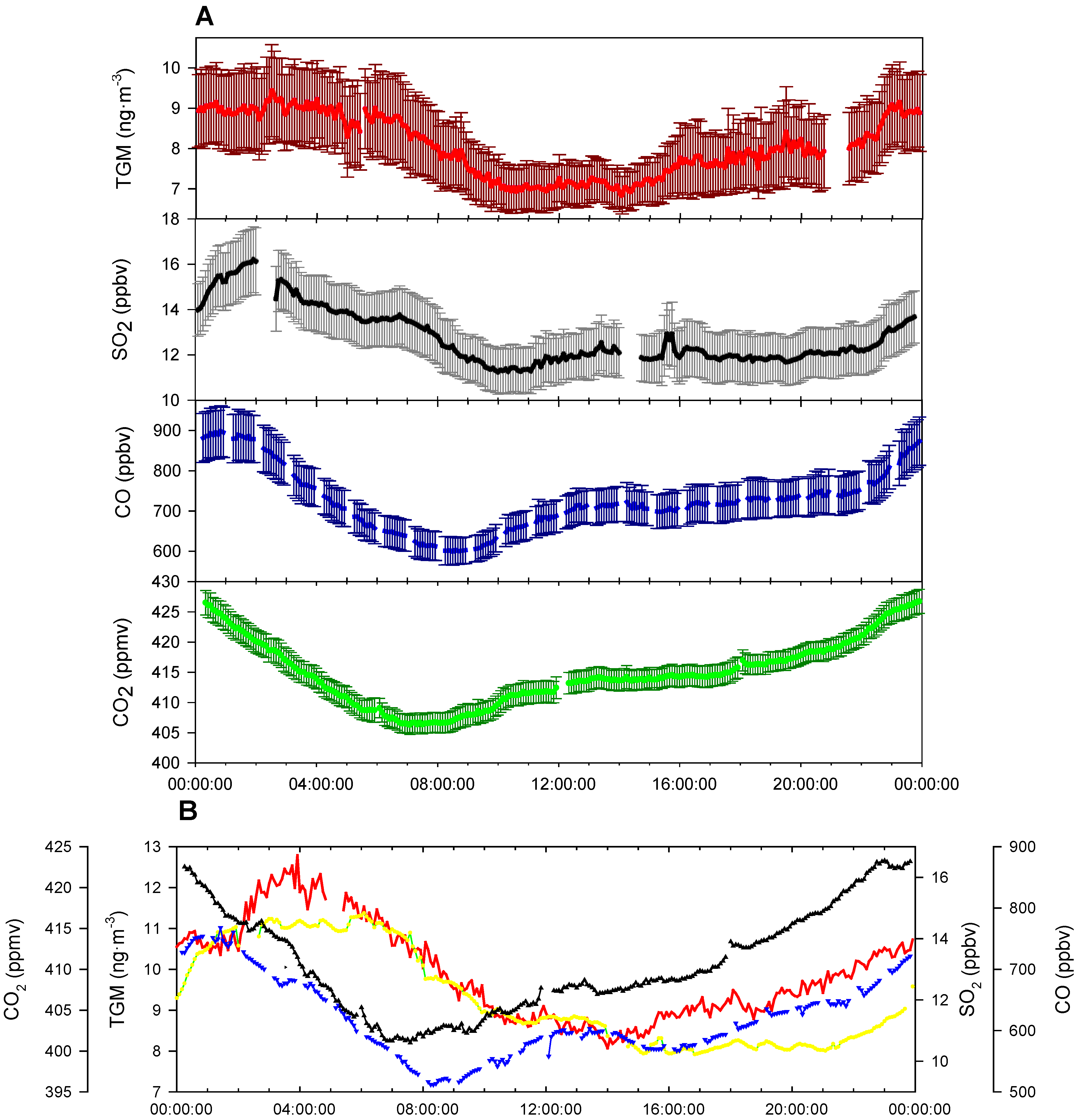
TGM shows a distinct diurnal pattern on a yearly averaged basis (Figure 8A). On average, the TGM concentrations are mostly constant from 0:00 to 6:00 UT with a small spike in concentrations at 2:00 UT. From 6:00 to 10:00 UT there is a drop of ~2.0 ng∙m⁻³ in TGM concentrations. Concentrations are rather constant from 10:00 to 13:00 UT. After 14:00, the concentrations in TGM begin to rise until 0:00, except for a small decline from 19:00 until 21:00 UT and a rapid rise between 22:00 and 23:00 UT. The nocturnal rise in TGM concentrations over 14:00–24:00 UT is indicative of the strong YRD emissions trapped under a low nocturnal boundary layer. The sources building under the nocturnal boundary layer are most likely of anthropogenic origin because legacy emission from soil and water are mediated by temperature and solar radiation [30], both of which are low at night. A significant correlation was observed between the nine-month average diurnal cycles of TGM and SO₂ with r² = 0.70, indicating the possibility of a strong source for both TGM and SO₂ on the nine-month scale. The source for such co-emission is most likely coal combustion considering that >70% of SO₂ emissions in the YRD region were from industrial combustion and power generation using coal in 2010 [31]. In contrast to the correlation of TGM and SO₂, the nine-month averaged diurnal cycles of TGM and other combustion products such as CO, NO_y, and CO₂ all have poor correlations with r² < 0.5, owing to a decline in concentrations of CO, NO_y, and CO₂ earlier in the morning and recovering sooner with near constant concentrations from 12:00 UT until 21:00 UT. This discrepancy indicates TGM has a different source profile than CO, CO₂, and NO_y and is likely co-emitted with SO₂. The line of best fit for the nine-month average diurnal cycles of TGM and SO₂ is:

(1)

The correlation slope translated to a molar ratio is 54.43 × 10⁻⁶ mol Hg∙mol⁻¹ SO₂. Normally trace gasses with such disparate lifetimes as TGM and SO₂ (six months to one year and ~one day respectively) would not facilitate a comparison to direct emissions. In this case the nine-month average diurnal cycle allows for a unique focusing on processes with a fine temporal resolution, in this case emissions. Furthermore, the close proximity of major point sources of both pollutants allowed sampling before major transformation or aging of the air mass could occur. The slope value can be compared to emission inventories of pollutants in the Yangtze River Delta to investigate YRD source types.

The SO₂ emissions given in Fu et al. [31] provide an estimate of 3.35 × 10¹⁰ mol total SO₂ emissions for the YRD region in 2010. Applying the molar ratio derived above, the total mercury emission from the YRD region would have been 366 tons or 1.8 × 10⁶ mol. This is an upper end estimate assuming no transformation or loss of SO₂ before measurement. A lower end estimate can be established by assuming that on a daily time scale, the temporal scale the correlation is based on, 63.2% of SO₂ was lost due to its 0.693-day half-life. Using this assumption of maximum daily loss before measurement the minimum emission of mercury would be 138 tons of Hg per year. Streets et al. [8] estimated that in 1999 the total mercury emission from Jiangsu and Zhejiang provinces, plus Shanghai, making up the YRD, were 42.16 tons or 2.1 × 10⁵ mol Hg, which is almost an order of magnitude lower than our upper end estimate and about three times smaller than our lower end estimate. Alternatively stated, emission inventories only account for as low as 12% to 31% of observed emissions. There are four possible reasons for this discrepancy: increased TGM emissions from 1999 to 2011, decreased sulfur dioxide emissions from 2010 to 2011, YRD emissions were much richer in mercury, and/or significant reemission of deposited mercury. The most likely scenario is a combination of mercury reemission as noted by Zhu et al. [9] and YRD emissions being enriched and, yet, underestimated in TGM compared to SO₂. Mercury emissions have most likely risen since 1999 due to continued and rapid economic development and increasing coal consumption. However, the existing emission inventories reported a meager increase in mercury emissions of 7.32% from 536 tons nationally in 1999 [8] to 575 tons in 2010 [4]. Additionally, emissions of sulfur dioxide appear to be declining according to Fu et al. [31] due to greater implementation of pollution controls. The opposing trends of increased TGM and decreased SO₂ emissions are not documented; therefore it is unknown if these trends constitute the order of magnitude required for the observed ratio of TGM to SO₂. Regarding the significance of legacy emissions, the rather strong reemission of deposited mercury, hypothesized by Zhu et al. [9] to contribute to enhance summertime TGM concentrations, was unlikely the majority of YRD emissions as would be required to make up the differential between observed emissions and inventory values. This is based on terrestrial reemissions constituting approximately 30% of annual global emissions [4].

Figure 8. (A) Nine-month average diurnal cycle of the sampling period of TGM (Red), SO₂ (Black), CO (Blue), and CO₂ (Green), with error bars representing 95% confidence interval. (B) Average diurnal cycle for summer season (June–August). The time axis is in UT, i.e., local time−eight hours.

Figure 8. (A) Nine-month average diurnal cycle of the sampling period of TGM (Red), SO₂ (Black), CO (Blue), and CO₂ (Green), with error bars representing 95% confidence interval. (B) Average diurnal cycle for summer season (June–August). The time axis is in UT, i.e., local time−eight hours.

Comparing seasonal differences, the rapid TGM peak seen in the nine-month average cycle (Figure 8A) occurs at approximately the same time, 22:00–23:00 UT near sunrise, in all seasons except summer. During the summer season, the increase was much delayed taking place at approximately 2:00 UT (Figure 8B), albeit earlier sunrises. The rapid enhancement of TGM occurs at near 10:00 AM local time, the approximate time of flux enhancements over soil in Canada during August, observed by Boudala et al. [30]. The time series of TGM flux from soil from Boudala et al. [30] was similar in shape to the diurnal cycle observed in Nanjing rapidly peaking at 10:00 AM, leveling off, and then declining. Although, the decrease in TGM concentrations comes much earlier in Nanjing likely as a result of an increased ventilation coefficient that peaks in the afternoon [25], and would not affect flux concentrations measured by a chamber as in Boudala et al. [30]. Legacy flux was unlikely the cause of the early morning peak throughout the rest of the year because the TGM peak was too early with respect to flux measurements and was concomitant with an SO₂ peak that has no photolytic mechanism in the troposphere [32]. The summer enhancement in Nanjing in mid-morning was ~2.0 ng∙m⁻³. Summer fluxes should be the greatest according to current understanding of mercury soil flux because the release of mercury appears to be a function of soil moisture, temperature [33]. Soil moisture should be greatest during this period due to the summer monsoon. The temperature and solar radiation reached the annual maximum [34]. It is highly likely that these three factors listed above interacted synergistically to increase soil evasion during the summer thereby contributing to the early 10:00 AM TGM peak observed in Figure 8B. Furthermore, mixing layer heights should theoretically affect all trace gases equivalently and land-sea winds should not affect the site due to being >200 km inland. The short and rapid enhancement seen in TGM in summer is also not followed by SO₂ as would be expected of coal emissions, which rules out coal combustion as a source. This enhancement was conceivably the release of legacy mercury as TGM, which would constitute 16% of peak concentrations in the summer diurnal cycle, far less than the global estimate of ~30% of mercury emissions being from natural or legacy fluxes. Additionally, this 16% of emissions is not enough to explain the discrepancy between observed and emission inventory based TGM concentrations.

Going back to the nine-month diel cycle, the drop in TGM concentrations comes in the afternoon, delayed several hours compared to the rise of the boundary layer; therefore it seems unlikely that downward mixing of less polluted air aloft caused the afternoon drop in TGM concentrations, unlike CO and CO₂. It appears that the concentrations of SO₂ and TGM were strongly controlled by the ventilation co-efficient which reaches its daily maximum in the afternoon [25] reasonably showing YRD emissions as the major source of TGM.

The emissions estimate above can be compared to the simulated mean mercury concentrations by Pan et al. [7] using the emissions inventory of Streets et al. [8], there is a clear underestimation of median mercury concentrations in Nanjing. The STEM-Hg∙model results estimate a median concentration of 1.6–1.7 ng∙m⁻³ [7], while Zhu et al. [9] found median mercury concentrations to be 6.2 ng∙m⁻³ [9]. Lin et al. used CMAQ-Hg to investigate the mass balance of mercury in East Asia and found higher concentrations of atmospheric mercury, ~3–4 ng∙m⁻³ [11], than Pan et al. [7], using similar emissions inventories, but TGM was still underestimated in comparison with measurements in Zhu et al. [9]. This discrepancy highlights further the fact that YRD TGM emissions are much greater than documented in Streets et al. for the region [8]. It is noted in Pan et al. [7] that discrepancies between the modeled and observed concentrations were in part due to the inaccurate model representation of dispersion from point sources. However, this problem should not affect mercury concentrations in the lower quartile of measurements, 4.5 ng∙m⁻³, which nearly triples the high estimate of 1.7 ng∙m⁻³ from Pan et al. The discrepancies between the emissions estimated in this study and models highlight the unique source profile in Nanjing and the possibility of large unaccounted for sources of TGM emissions in the YRD.

2.3. Peak Concentrations

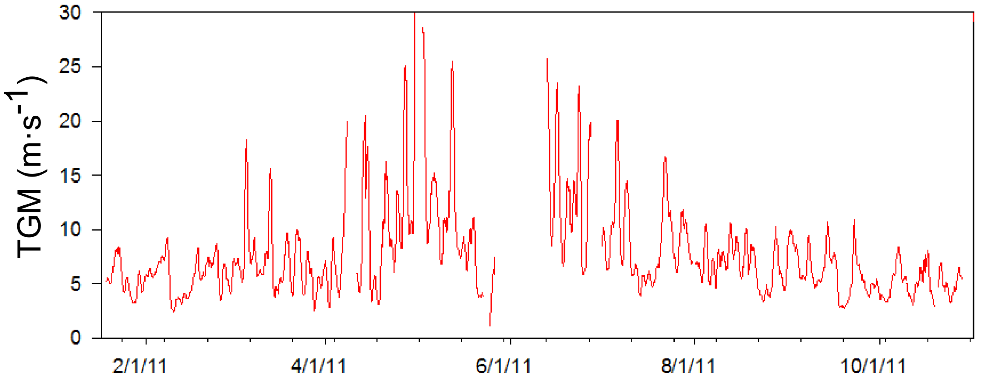
Throughout the measurement period TGM concentrations reached levels that were extraordinarily high compared to measurements made in North America and Europe [35]. In order to more clearly understand the sources and causes of these high concentrations, an episodic high concentration of TGM was defined for each season. One-day moving averages were used to smooth out diurnal variation, which was found to be the most frequent controlling interval based on a power spectrum analysis of the data (not shown). When the one-day moving average concentration of TGM (Figure 9) exceeded the seasonal 90th percentile value it was considered an episode of high TGM concentrations. The seasons were defined as January and February for winter; March, April, and May for spring; June, July and August for summer; and September and October for fall. The episode concentration criterion was highest during the summer months at 17.1 ng∙m⁻³ and lowest in winter at 8.3 ng∙m⁻³. As a result, 20 high TGM episodes were identified in 2011 and are listed in Table 1.

Once the episodes were determined they were plotted along with the time series of CO, SO₂, O₃, NO_y, wind speed, and direction. Using these four trace gases and wind, qualitative relationships between traces gases and peak TGM concentrations were determined. When TGM concentrations reached episode concentrations accompanied by spikes in urban tracers such as CO and SO₂ under weak wind conditions (wind speed <2 m∙s⁻¹), it was hypothesized that the source of higher TGM concentrations was the anthropogenic YRD emissions. Using this system, 50% of the episodes appeared due to stagnant conditions, including low O₃ episodes (Table 1) and buildup of YRD sources in Nanjing. The largest controlling factor of TGM and high TGM concentrations was YRD emissions, while other controlling factors include the monsoon and transport from other source regions.

Figure 9. The graph above shows the time series of the one-day moving average of mercury concentrations based on five-minute data.

Figure 9. The graph above shows the time series of the one-day moving average of mercury concentrations based on five-minute data.

Table 1. The table contains mercury episodes in chronological order. The date of the episode is the point of the peak. The concentration in column three is the highest achieved during a 24-hour moving average. The coincident peaks were qualitatively assigned from other trace gases. The other columns are the defining characteristics of the episode, the type or classification. The last three columns are the slope of the linear regression of the trace gas vs. mercury data from the 72 hours around the episode. Only slopes of correlations with an r² > 0.2 and p-value < 0.001 were included.

#	Date	24 Hr Moving avg Peak	Coincident Peaks	Characteristics	Classification	TGM-CO Slope	TGM-SO2 Slope	TGM-NOy Slope
1	1/23	8.4	CO, SO2	Low winds	Local	0.003	N/A	0.049
2	2/7	8.8	CO, SO2, O3	Low winds High O3	Local	0.003	0.074	0.063
3	2/17	8.3	CO, SO2	Low winds	Local	0.004	0.141	0.051
4	2/24	8.7	CO, SO2, O3	Low winds High O3	Local	0.005	0.221	0.057
5	3/5	18.2	CO, SO2	Low Winds	Low O3	0.016	0.480	0.240
6	4/7	19.5	CO, SO2, O3	Low winds High O3	Local	0.017	0.382	0.242
7	4/13	20.5	CO, Slight SO2	Low winds	Local	N/A	N/A	0.253
8	4/20	16.2	CO, SO2	Low winds & Sudden drop in O3	Low O3	0.008	0.546	0.195
9	4/26	25.0	None	High Winds & Other Gases low	Transport	N/A	N/A	N/A
10	4/30	53.9	None	High Winds & Other Gases low	Transport	N/A	N/A	N/A
11	5/12	25.5	SO2, O3	Low CO, SO2 but elevated spiking O3 and moderate winds	Transport	N/A	N/A	N/A
12	6/12	65.5	CO, SO2 After TGM	Low Winds	Monsoon	0.059	N/A	N/A
13	6/16	23.5	CO, SO2	Low winds	Monsoon	N/A	N/A	N/A
14	6/23	23.1	CO, SO2	Low wind	Monsoon	0.012	0.622	N/A
15	6/27	19.9	CO, SO2, O3	Trace gasses and Low winds	Monsoon	0.011	0.914	0.377
16	7/6	20.1	All	Low winds	Monsoon	N/A	1.076	0.151
17	7/22	16.6	All	Trace Gases peak and Low winds	Monsoon	N/A	0.451	N/A
18	9/1	10.0	All peak after	O3 Peaks and SO2 after low wind speeds	Local	N/A	N/A	N/A
19	9/13	10.7	None	CO drops O3 flat lines after peak SO2 drops Winds are moderate	Transport from Hangzhou	N/A	N/A	N/A
20	9/22	10.9	CO, O3	Low winds, O3 peaks after CO peaks with TGM	Local	N/A	N/A	N/A

Table 1. The table contains mercury episodes in chronological order. The date of the episode is the point of the peak. The concentration in column three is the highest achieved during a 24-hour moving average. The coincident peaks were qualitatively assigned from other trace gases. The other columns are the defining characteristics of the episode, the type or classification. The last three columns are the slope of the linear regression of the trace gas vs. mercury data from the 72 hours around the episode. Only slopes of correlations with an r² > 0.2 and p-value < 0.001 were included.

#	Date	24 Hr Moving avg Peak	Coincident Peaks	Characteristics	Classification	TGM-CO Slope	TGM-SO2 Slope	TGM-NOy Slope
1	1/23	8.4	CO, SO2	Low winds	Local	0.003	N/A	0.049
2	2/7	8.8	CO, SO2, O3	Low winds High O3	Local	0.003	0.074	0.063
3	2/17	8.3	CO, SO2	Low winds	Local	0.004	0.141	0.051
4	2/24	8.7	CO, SO2, O3	Low winds High O3	Local	0.005	0.221	0.057
5	3/5	18.2	CO, SO2	Low Winds	Low O3	0.016	0.480	0.240
6	4/7	19.5	CO, SO2, O3	Low winds High O3	Local	0.017	0.382	0.242
7	4/13	20.5	CO, Slight SO2	Low winds	Local	N/A	N/A	0.253
8	4/20	16.2	CO, SO2	Low winds & Sudden drop in O3	Low O3	0.008	0.546	0.195
9	4/26	25.0	None	High Winds & Other Gases low	Transport	N/A	N/A	N/A
10	4/30	53.9	None	High Winds & Other Gases low	Transport	N/A	N/A	N/A
11	5/12	25.5	SO2, O3	Low CO, SO2 but elevated spiking O3 and moderate winds	Transport	N/A	N/A	N/A
12	6/12	65.5	CO, SO2 After TGM	Low Winds	Monsoon	0.059	N/A	N/A
13	6/16	23.5	CO, SO2	Low winds	Monsoon	N/A	N/A	N/A
14	6/23	23.1	CO, SO2	Low wind	Monsoon	0.012	0.622	N/A
15	6/27	19.9	CO, SO2, O3	Trace gasses and Low winds	Monsoon	0.011	0.914	0.377
16	7/6	20.1	All	Low winds	Monsoon	N/A	1.076	0.151
17	7/22	16.6	All	Trace Gases peak and Low winds	Monsoon	N/A	0.451	N/A
18	9/1	10.0	All peak after	O3 Peaks and SO2 after low wind speeds	Local	N/A	N/A	N/A
19	9/13	10.7	None	CO drops O3 flat lines after peak SO2 drops Winds are moderate	Transport from Hangzhou	N/A	N/A	N/A
20	9/22	10.9	CO, O3	Low winds, O3 peaks after CO peaks with TGM	Local	N/A	N/A	N/A

2.3.1. Monsoon Effects on TGM

The summer monsoon season in the YRD region comes with the shifting of prevailing flows at 850 hPa from the north, during most of the year, to south during mid-May [16]. The winds at the surface level shift to east-southeast and at 500 hPa westerlies are observed. As the flows shift, rain bands move northward in early June signaling the beginning of the Meiyu season (i.e., rainy season) in the YRD. The monsoon system sets up as a quasi-stationary front with an average eight day intervals of passage [16]. These slow moving systems in the YRD in addition to larger summertime sources, such as biomass burning [15], increased baseline due to higher revolatilization [9], and changes to summer weather due to biomass burning [18] may help explain the extraordinarily high concentrations of TGM during the mid-May–July monsoon season. The observed enhancement of TGM in Nanjing stands in contrast to other regions of China, such as the PRD, where the monsoon brought a decrease in atmospheric mercury concentrations over the season [17].

When the region was under the southwesterly flow at 850 hPa during∙mid-May to July 2011, TGM appears to spike. Spikes in TGM concentrations reaching high episode concentrations occurred on 12 June 2011, 16 June 2011, 23 June 2011, 27 June 2011, 6 July 2011, and 22 July 2011 corresponding to episodes numbered 12–17 in Table 1. In contrast, a drop in TGM concentrations most notably on background episode on 13 July 2011 discussed above was caused by strong flows from the southeast.

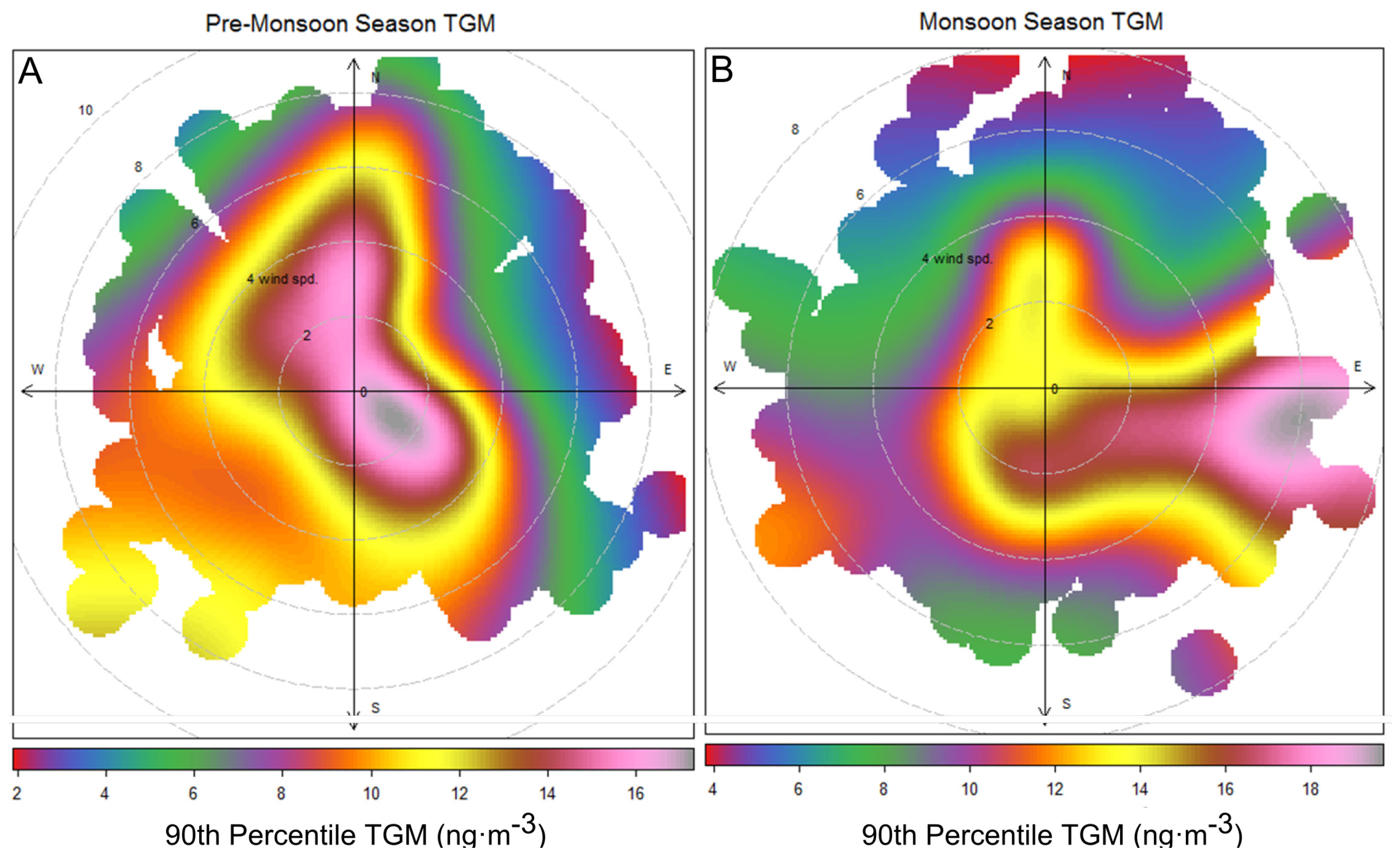
Figure 10. TGM concentrations were binned by wind speed and direction. The 90th percentile was then plotted for (A) April–15 May, 2011 and (B) 16 May 2011–July 2011.

Figure 10. TGM concentrations were binned by wind speed and direction. The 90th percentile was then plotted for (A) April–15 May, 2011 and (B) 16 May 2011–July 2011.

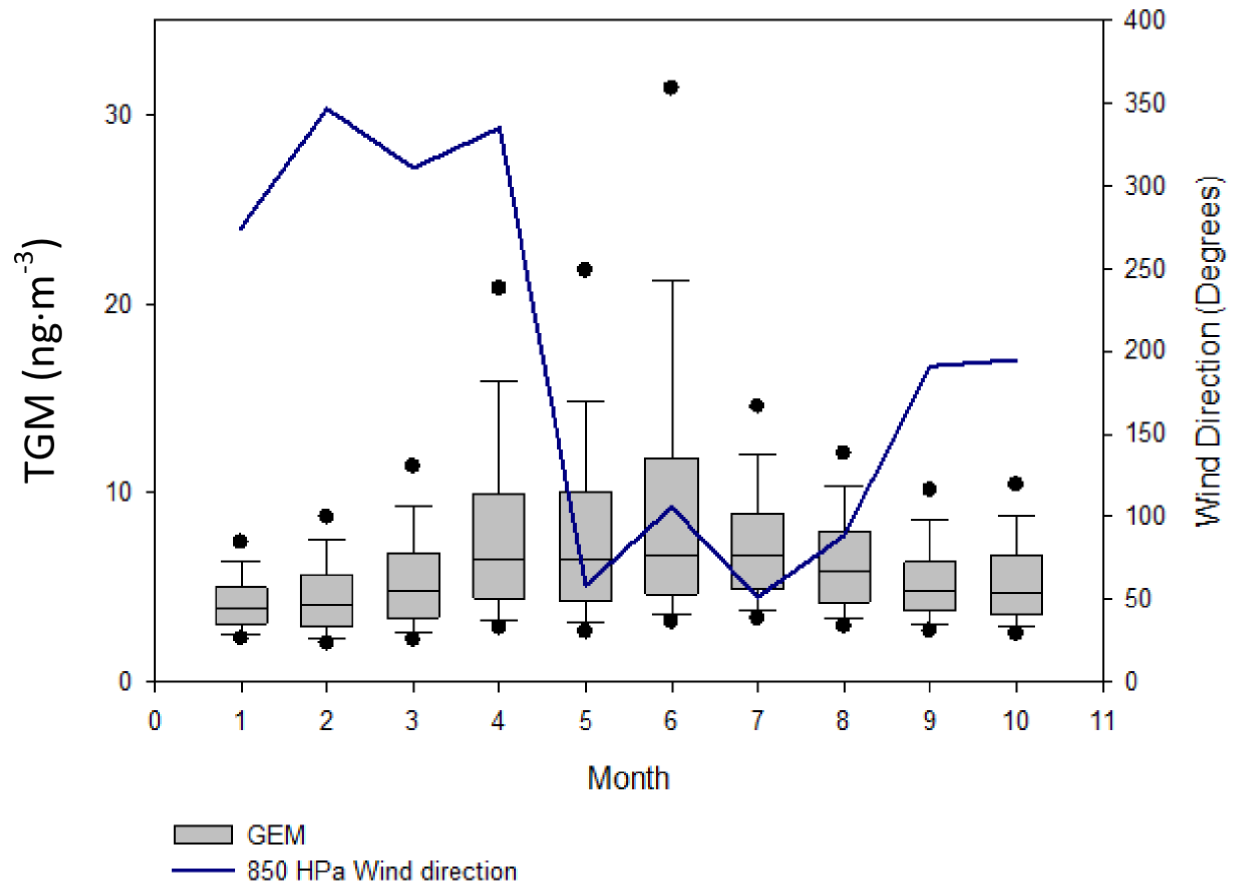
However, the arrival of monsoon season is not timed exactly with the increase in TGM values. The monthly median TGM value is elevated in April–May (Figure 7) before the flow shift in mid-May. During April and the first half of May elevated TGM concentrations correspond with low wind speeds or northerly winds (Figure 10A), and contrast this with the second half of May, June, and July where the highest TGM came from easterly directions (Figure 10B). In June, the 10th, 75th, and 90th percentile values are much higher than in May indicating high episodic and baseline concentrations of TGM in June. The monsoon season may be only enhancing episodic concentrations of TGM during the summer while higher summer time temperatures and biomass burning raise median values in April through July [9,15].

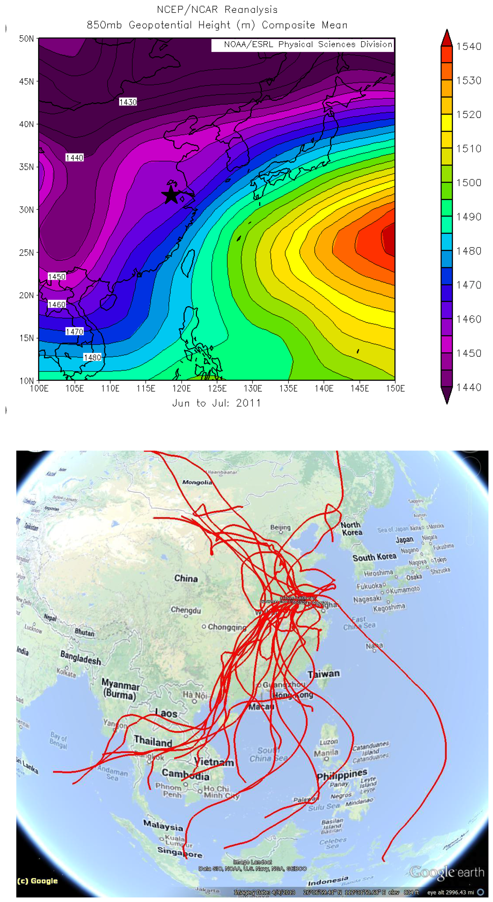
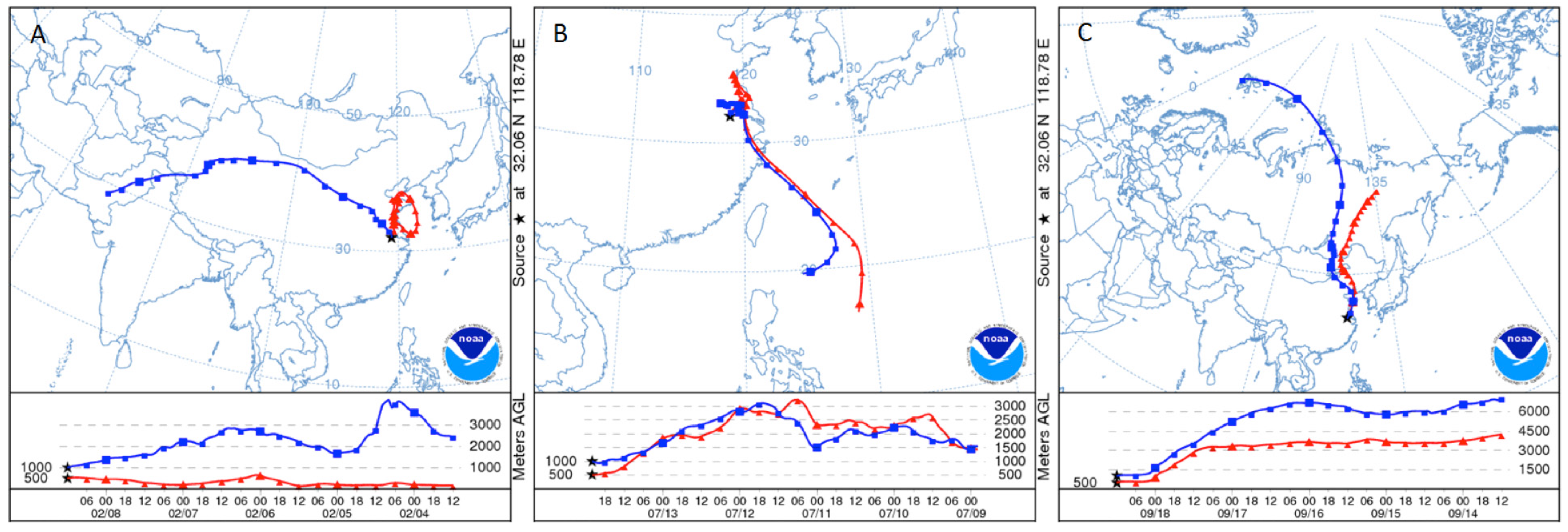
The extraordinary concentrations of TGM observed during June of 2011(Figure 8, Figure 9 and Figure 10B) were further investigated. The map of average geopotential height for 850 hPa shows prevalence of southwesterly flows in the YRD resulting from the low pressure system north of China and the subtropical high over the western Pacific during June and July of 2011 (Figure 11A). To further investigate the effects of the monsoon, five-day backward trajectories for 7 June 2011, through 7 July 2011 starting at 1,500 m were plotted (Figure 11B). Figure 11B illustrates that 47% of the trajectories originated from southern China and the Indochina peninsula. Looking exclusively at episodically high day TGM concentrations there appear to be three ways in which TGM is enhanced in the region during the monsoon.

Figure 11. Synoptic-scale flows during the monsoon season (A) Geopotential height for June and July, 2011, at the 850 hPa level (B) Five-day backward trajectories from Nanjing, China for 7 June 2011 through 7 July 2011 ending at 1500 m.

Figure 11. Synoptic-scale flows during the monsoon season (A) Geopotential height for June and July, 2011, at the 850 hPa level (B) Five-day backward trajectories from Nanjing, China for 7 June 2011 through 7 July 2011 ending at 1500 m.

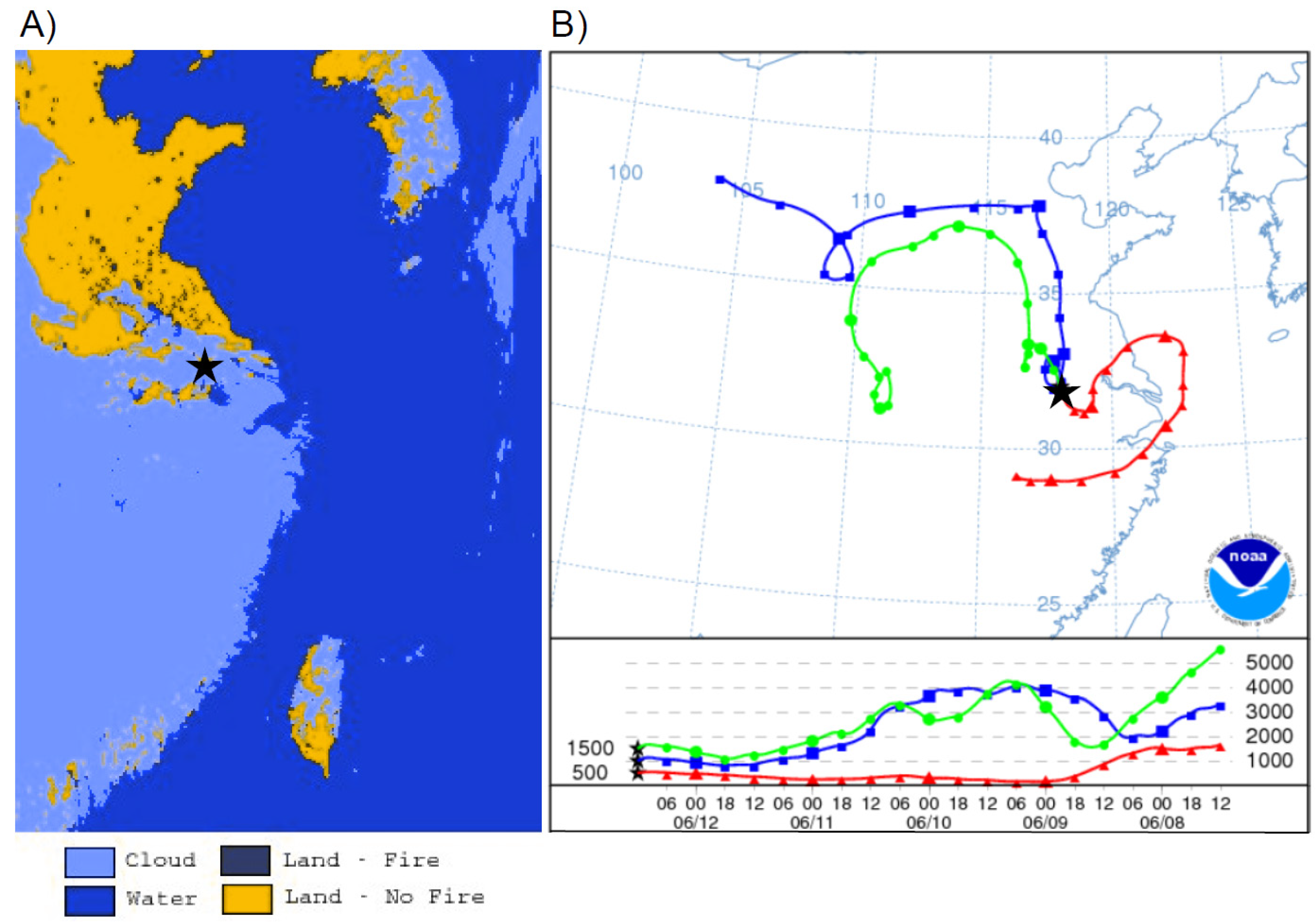
The first monsoon season episode happened on the 12 June episode with stagnant backward trajectories showing air masses building up within the YRD (Figure 12B). Although there was a lack of correlation during this time period between TGM and SO₂ or NO_y, which was counterintuitive given the apparent urban nature of the episode, there was a strong correlation between TGM and CO with a slope of 0.059 ng∙m⁻³ TGM ppbv⁻¹ CO. In addition, the Moderate Resolution Imaging Spectroradiometer (MODIS) fire map shown in Figure 11A indicates a large number of agricultural fires, a source of CO and TGM, in the region possibly causing an inversion as noted by Ding et al. [18] that could build up TGM and CO concentrations in the YRD. This is especially interesting given the much higher CO and TGM correlation coefficient during this particular episode compared to other episodes in Table 1.

Figure 12. On 12 June 2011 (A) Fires from MODIS (defined in text) five-min Fire product V2 and (B) a five-day backward trajectory from Nanjing starting at the 500, 1000, and 1500 m level at 12:00 UT. The star ( ) indicates the location of Nanjing.

Figure 12. On 12 June 2011 (A) Fires from MODIS (defined in text) five-min Fire product V2 and (B) a five-day backward trajectory from Nanjing starting at the 500, 1000, and 1500 m level at 12:00 UT. The star ( ) indicates the location of Nanjing.

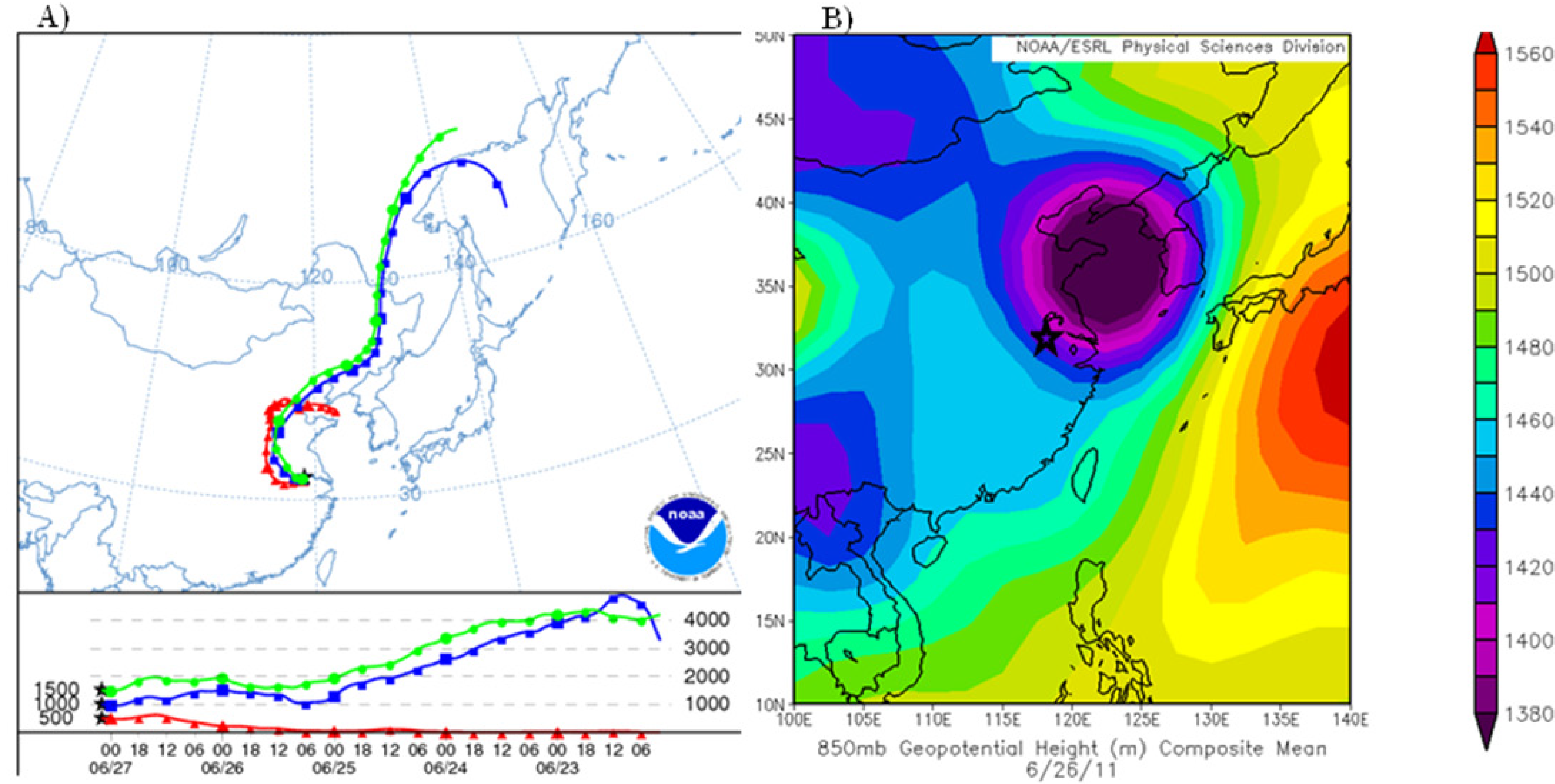
The second type was due to passing low-pressure systems causing a northerly circulation from the Beijing region, this occurred on 27 June. There was a low-pressure system on 26 June 2011 before concentrations of TGM began to rise (Figure 13B). The accompanying HYSPLIT plot (Figure 13A) illustrates air coming from the industrialized north of China ending at the time of the TGM peak 02:00 UT on 27 June. During the 27 June episode the correlations of TGM with CO, SO₂, and NO_y were good indicators of a strong urban source of TGM.

Figure 13. (A) Five-day backwards trajectory from Nanjing ending on 27 June 2011, at 02:00 UT. (B) NCEP/NCAR reanalysis at 850 hPa showing low-pressure system that passed over Nanjing on 26 June 2011 and imported high mercury on 27 June 2011.

Figure 13. (A) Five-day backwards trajectory from Nanjing ending on 27 June 2011, at 02:00 UT. (B) NCEP/NCAR reanalysis at 850 hPa showing low-pressure system that passed over Nanjing on 26 June 2011 and imported high mercury on 27 June 2011.

The third type of monsoon season episode is due to flows from the south southwest. The PRD was identified as the largest emissions region of TGM in the last published emissions inventory for China [8] and therefore could have an effect on the mercury concentrations in Nanjing. Looking at the HYSPLIT model plot of 7 June through 7 July (Figure 10B) it is clear that there is a common southwesterly flow during this period at the 1500 m level (Figure 10A). Compared with the 850 hPa geopotential height map for May (not shown), it is clear that air more likely arrived from the southwest during the summer monsoon season. This seasonal enhancement is in stark contrast to the effect the monsoon had on mercury concentrations in the PRD region as noted by Chen et al. 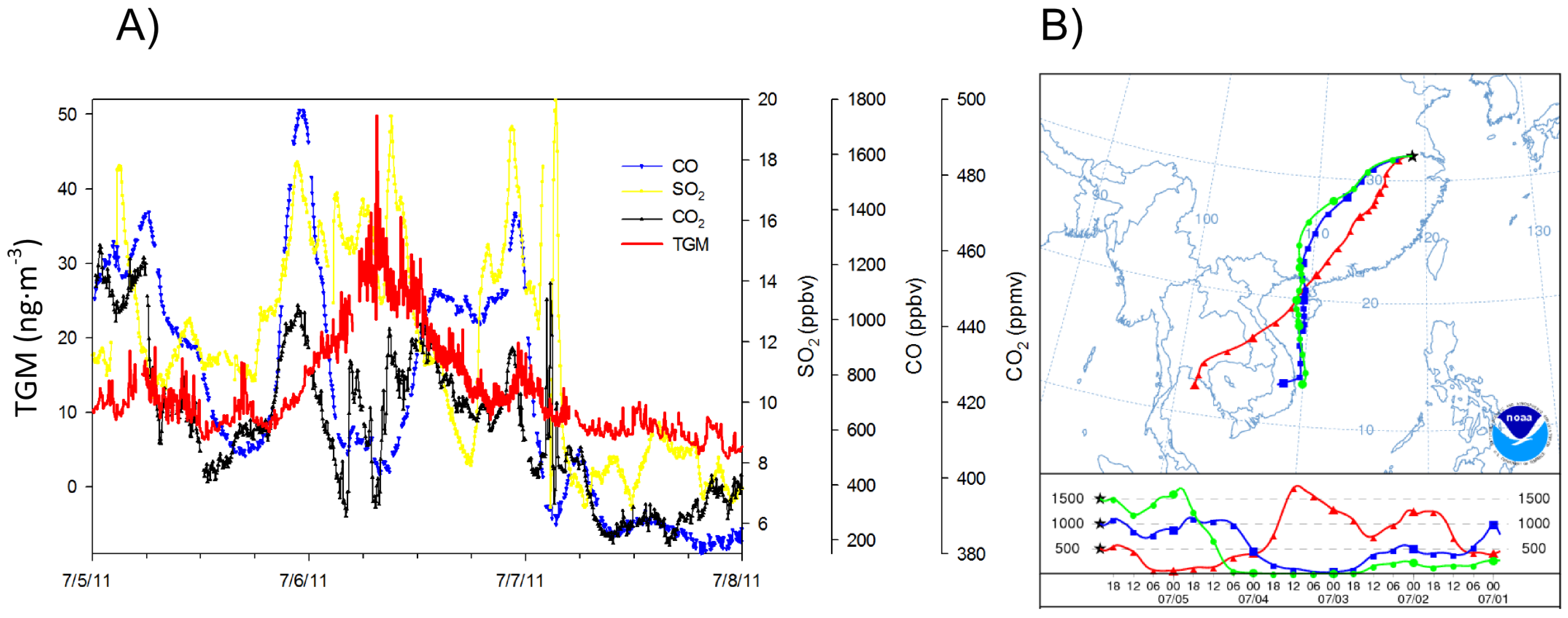[17], where mercury was diluted by relatively clean marine air masses entering the region via monsoonal southwesterly flows. A good example of an episode of high TGM concentrations transported from the southwest occurred on 6 July 2011. During this occurrence the wind speed was sustained at approximately 2 m∙s⁻¹ during the whole episode. Additionally there was a spike in CO and CO₂ (Figure 14A) that preceded the TGM spike, most likely due to morning rush hour, as the peak occurred at approximately 7:00 a.m. local time while the HYSPLIT trajectory (Figure 14B) was very similar to seasonal average. Moreover, wind speed and direction did not shift much, indicating consistent flows. All of these illustrate the possibility of transport from a strong source region southwest of the observation site.

The monsoon season in the YRD appears to have a very large impact on TGM concentrations. There are three separate ways in which TGM concentrations were enhanced these were: Biomass induced, northern transport, and southern transport. A fourth possible mechanism is increased legacy flux due to greater soil moisture discussed above. These factors in addition to the stronger summer sources noted in Lin et al. [11] contribute to a summertime concentration in the YRD that was anomalously large in comparison to Northern Hemispheric background.

Figure 14. The high TGM episode on 6 July represented in (A) time series and (B) with the five-day backwards NOAA HYSPLIT plot at 500, 1,000, and 1,500 m.

Figure 14. The high TGM episode on 6 July represented in (A) time series and (B) with the five-day backwards NOAA HYSPLIT plot at 500, 1,000, and 1,500 m.

2.3.2. TGM Peaks during Low Ozone

There were two episodes on 5 March and 20 April, denoted as episodes #5 and #8 in Table 1, where O₃ depletion was coincident with spikes in TGM concentrations over approximately a twelve hour period. On these occasions concentrations in SO₂, NO_y, and CO all became elevated in tandem with TGM concentrations, while O₃ concentrations remained under 20 ppbv. These episodes were also coincident with slow winds under 2 m∙s⁻¹ increasing buildup in the YRD, while Nanjing sat between fronts, similar to local episodes discussed below. The exceptional part about these episodes is the low O₃ that accompany them. The depressed concentrations of O₃ are not seen in other similar episodes.

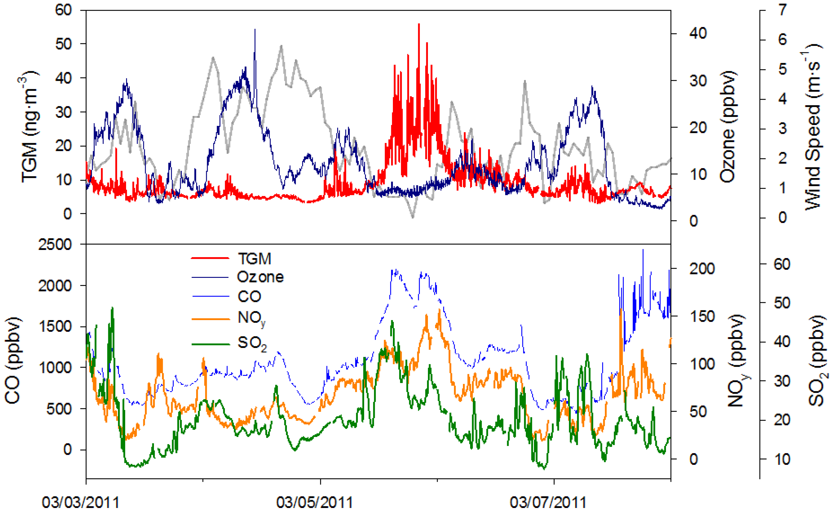
Figure 15. Time series of TGM, O₃, CO, NO_y, SO₂, and wind speed (gray) over the period 3 March 2011 through 7 March 2011. This represents episode #5 in Table 1.

Figure 15. Time series of TGM, O₃, CO, NO_y, SO₂, and wind speed (gray) over the period 3 March 2011 through 7 March 2011. This represents episode #5 in Table 1.

The cause of low O₃ on 5 March 2011, appears to be titration by NO based on elevated concentrations of NO_y timed with the O₃ drop (Figure 15). A time series of TGM, O₃, CO, NO_y, SO₂, and wind speed can be seen in Figure 15. The low wind speeds (<2 m∙s⁻¹) during peak TGM concentrations coincide with increasing radiation flux to a maximum of 271 W∙m⁻² during the O₃ minimum on 5 March 2011. While O₃ rose the next day, 6 March 2011, the peak radiation flux was much lower at 65.6 W∙m⁻². On the previous day, 4 March 2011, radiation flux reached over 500 W∙m⁻² and the O₃ concentration was much higher near 30 ppbv.

In contrast to 5 March, low O₃ on 21 April 2011 seems to be linked mostly to a very low radiation flux of 91.4 W∙m⁻². This is coincident with low winds and high concentrations of urban tracers that indicate urban pollution. In addition, this area is under the influence of a low pressure system bringing in marine air and cloud cover.

Low O₃ only occurred in these two instances out of all of the high TGM episodes. It appears to be a coincident timing with decreased O₃ and a period of stagnation in the boundary layer and cloudy conditions, based on the radiation data. As both of these are a function of solar radiation, it seems unusual that this sort of stagnant, low O₃, high TGM episode only occurred on the two occasions listed above. The anomalous drop in O₃ may be due to mobile sources, which are known to be a strong source of NO. The other possible source of titrating nitrogen may be plumes of industrial and electrical boilers since these two sources account for over half of the NO_x emissions in the YRD [31]. Furthermore, the linear correlation slope values between TGM and NO_y were unusually high at 0.24 ng∙m⁻³ TGM ppbv⁻¹ NO_y on 5 March, 2011 and 0.20 ng∙m⁻³ TGM ppbv⁻¹ NO_y on 20 April compared to 0.054 ng∙m⁻³ TGM ppbv⁻¹ NO_y during the entire winter, indicating the increased importance of NO_y in the atmospheric composition and therefore as a titrant. The r² value for the correlation of NO_y and TGM was also high at 0.51 on 5 March 2011. Additionally, there was a linear correlation of TGM and SO₂ during both episodes showing a high slope value indicating a strong source of TGM with SO₂. Taken together these seem to indicate a possible plume from industrial or electrical boilers rather than mobile combustion as would normally be assumed in such a low O₃ environment. Overall, these episodes seem to speak to the importance of stagnant meteorology increasing TGM and other pollutants, such as NO_y and CO, while titrating or removing O₃ although YRD source density makes any conclusions about a single cause of low O₃ difficult.

2.3.3. Transport of TGM from Non-Urban Sources

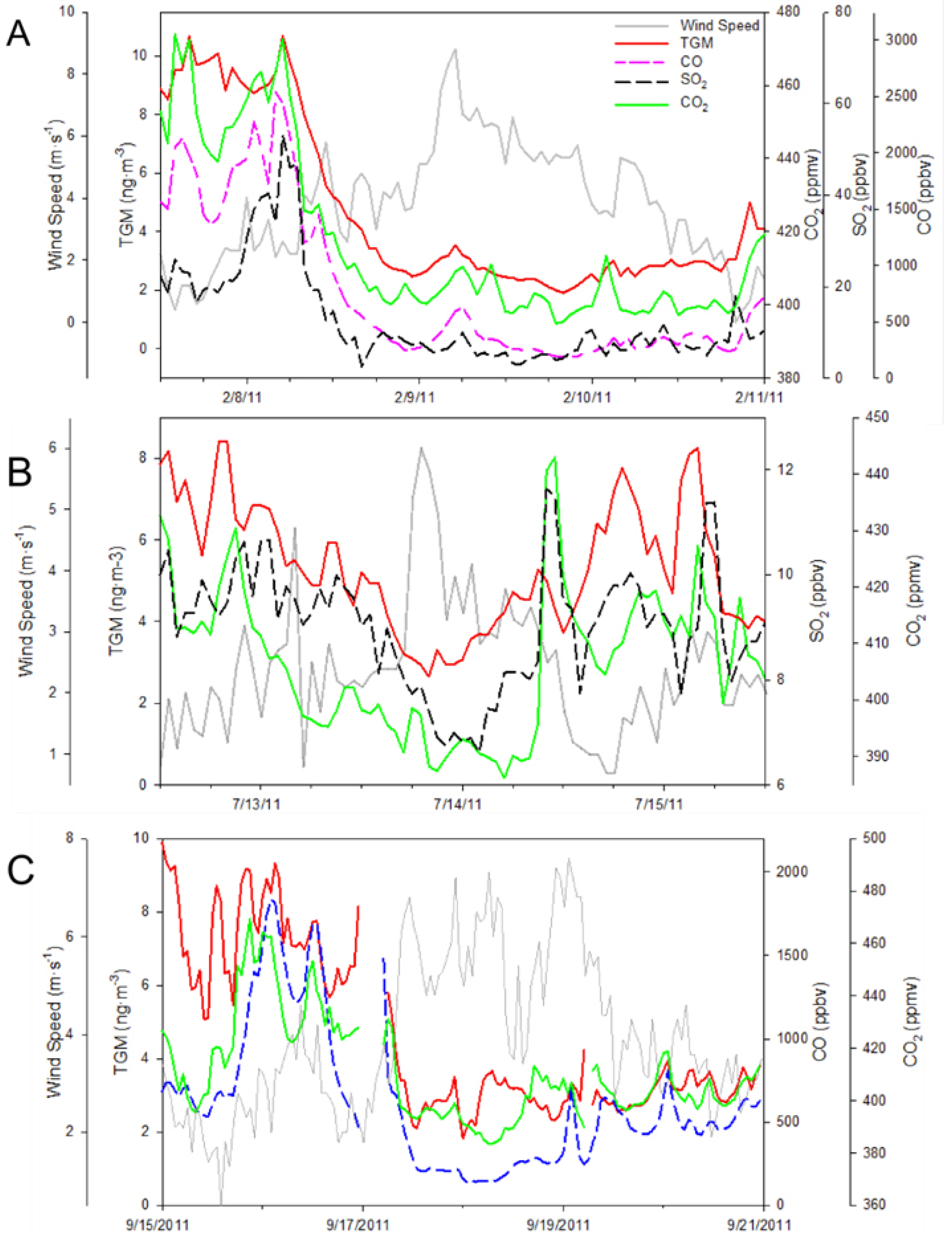
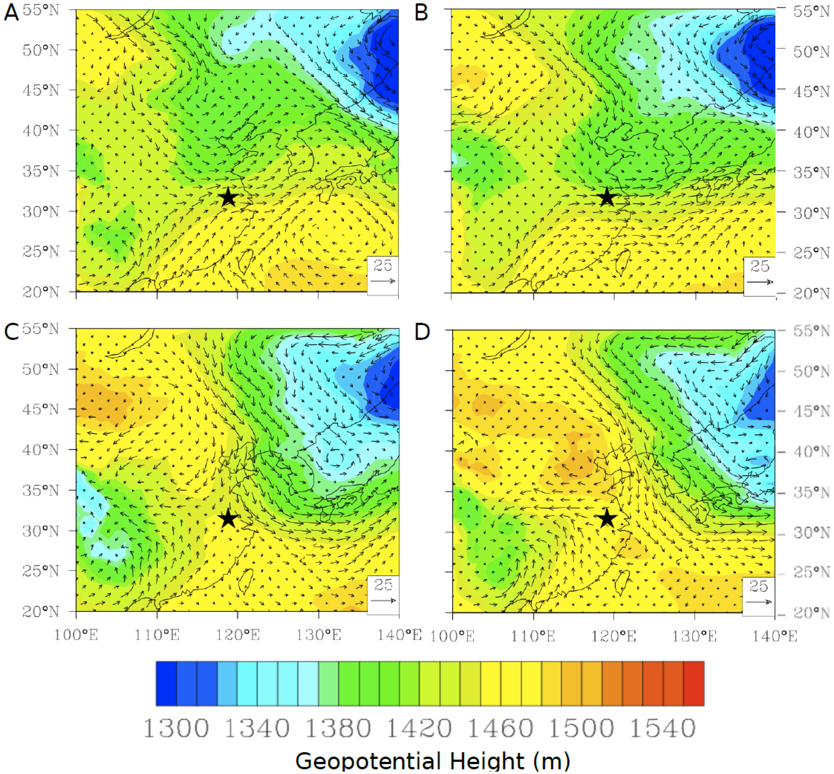
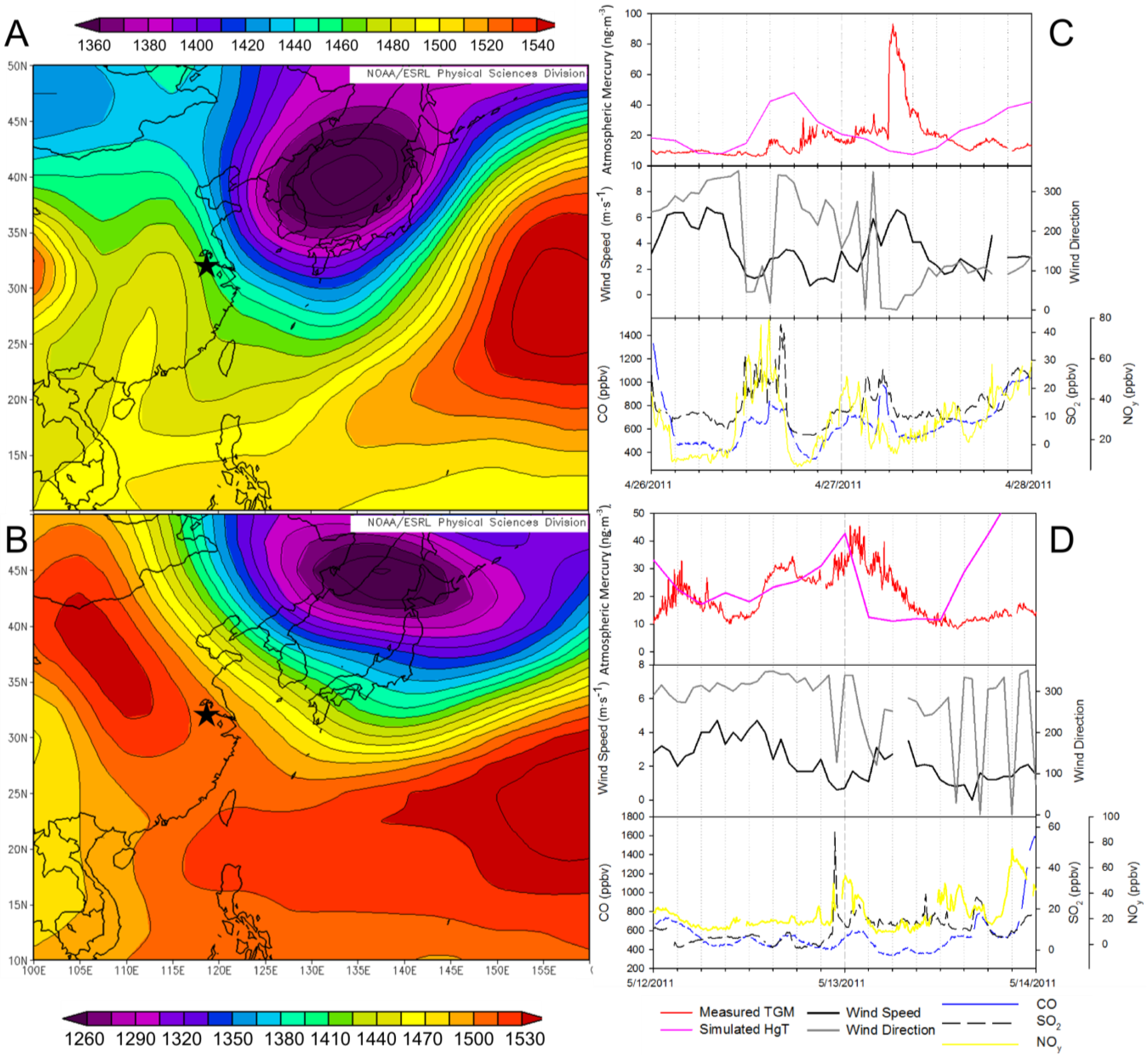
Three episodes on 26 April, 13 May, and 13 September 2011, appear to be due to transport. The spring episodes occurred with no correlated trace gases and during periods of high winds in contrast to most localized episodes coincident with wind speeds less than 2 m∙s⁻¹. Further investigation of the geopotential height at 850 mbar height using daily NCEP/NCAR reanalysis data shows that in both cases during the spring there was a low pressure system passing north of Nanjing over the Korean peninsula and into the Sea of Japan (Figure 16A,B). The strength of the gradient flow varies from episode to episode. On 27 April 2011, Nanjing was immediately under the influence of strong gradient flows formed by a high-pressure ridge west of Nanjing and a strong low pressure system to the northeast (Figure 16A). In comparison, on 13 May 2011, Nanjing was sitting outside of strong gradient flows as shown in Figure 16B. These meteorological systems appear to transport polluted air masses rich in mercury from the heavily industrialized north of China into Nanjing, although the lack of correlation with any other trace gas (Figure 16C,D) indicates otherwise. Possible explanations for the lack of correlation are industrial sources that intentionally use elemental mercury such as compact florescent light manufacturing, artisanal small scale gold mining, wet deposition or removal of more reactive gases, e.g., SO₂ and NO_y, and/or transport from rural areas.

Compact florescent light and battery manufacturing are major contributors to mercury emissions in the PRD region of China [36]. These industrial emissions appear to be due to accidental release of mercury used in the final product, not combustion and so therefore are not coincident with combustion tracers such as CO, SO₂, and NO_y. However, such industrial sites are expected to be collocated with urban emissions. The fact that while mercury concentrations spiked, urban tracers were flat, indicates a non-urban source of emissions.

Wet deposition of the more reactive gases during transport is unlikely since NCEP/NCAR reanalysis data for all three occasions shows no precipitation in and around Nanjing or north of the location. Additionally, if the mercury were of urban origin and the other trace gases were removed by a process that acted on reactive gases, then CO should remain intact as a tracer of urban emissions. In the case of these episodes it is unlikely that the mercury is of urban origin because of lack of high concentrations of CO, a relatively long lived and insoluble gas.

Rural sources of mercury in China generally include biomass burning and artisanal mining [4,15]. Biomass burning of fields and crop residue is a source of mercury in China, especially in Shandong, north of Nanjing, and the Jiangsu provinces [8,15]. Biomass burning as an inefficient combustion source is generally considered to emit CO which does not spike during the three episodes considered here. In addition to the lack of correlation with CO, episodes in the spring occurred before summer field burning began [18], ruling out biomass burning as the source of these episodes. Artisanal mining can produce mercury emissions, ~45% of the released mercury is atmospheric, through the use of mercury amalgamation to recover gold from ore and is the single largest source of atmospheric mercury emissions in China, making up ~29% [4]. Although mercury amalgam processes are illegal in China, they are still in use [14], and, thus, many of these artisanal mining sources have not been included in emission inventories. Artisanal mining is greatest in Hebei and Shandong both due north of Nanjing [14]. In Figure 16, for both episodes there is a common theme of air masses passing over these provinces before reaching Nanjing. Additionally there are north to northwesterly flows (Figure 16C,D). Furthermore, 27 April reached higher TGM concentrations and had a stronger gradient and therefore winds. In comparison, TGM concentrations on 13 May did not reach as extraordinary concentrations, while the pressure gradient was not located directly over Nanjing and consequently wind speeds facilitating transport to Nanjing were not as fast. The difference in TGM concentrations corresponds to the strength of transport phenomena; therefore transport from the Shandong and Hebei are likely candidates for the source of the high TGM concentrations during these episodes. Artisanal mining would explain why TGM concentrations spiked while combustion gases concentrations stayed low and wind speeds rose (Figure 16C,D).

To determine if TGM concentrations were a function of known emission sources the concentration of TGM were simulated using Lagrangian particle dispersion modeling (LPDM). Simulated mercury concentrations do not peak simultaneously with the observed TGM concentrations (Figure 16C,D). In the 27 April 2011instance the observed peak comes arrives between the two simulated peaks and was much greater in magnitude. On 13 May 2011the simulated peak comes before the actual TGM peak but was approximately equal in magnitude. On 13 May 2011 the simulated mercury peak declines to the baseline within 3 hours, whereas the observed decrease lasted 12 hours. The simulations employed gridded emissions in the AMAP/UNEP for the year 2010. The fact that the TGM concentrations are not captured in the model indicates missing∙mercury sources in emission inventories, such as artisanal mining sources in and around China. Such evidence seems to support undocumented artisanal mines in the provinces north of Nanjing releasing TGM that was transported on a regional scale to Nanjing.

Figure 16. The geopotential height at 850 hPa over East Asia from NCEP/NCAR reanalysis for (A) 27 April 2011 and (B) 13 May 2011. A time series of measured TGM (red), Flexpart simulated TGM (magenta), wind speed (black), wind direction (grey), CO (blue), NO_y (yellow), and SO₂ (black dash) for (C) 26 and 27 April 2011, (D) 12 and 13 May 2011. The star ( ) indicates the location of Nanjing.

Figure 16. The geopotential height at 850 hPa over East Asia from NCEP/NCAR reanalysis for (A) 27 April 2011 and (B) 13 May 2011. A time series of measured TGM (red), Flexpart simulated TGM (magenta), wind speed (black), wind direction (grey), CO (blue), NO_y (yellow), and SO₂ (black dash) for (C) 26 and 27 April 2011, (D) 12 and 13 May 2011. The star ( ) indicates the location of Nanjing.

2.3.4. Localized Emissions

This grouping of episodes includes 50% of episodes and generally happened during periods of low wind speed (<2 m∙s⁻¹). There is a diversity of slope values of correlations between TGM and other tracers (Table 1). The values for localized episodes with an r² > 0.2 between CO and TGM ranged from 0.003 to 0.017 ng∙m⁻³ TGM ppbv⁻¹ CO. For SO₂ the slope values reported above the criteria listed previously range from 0.074 ng∙m⁻³ TGM ppbv⁻¹ SO₂ to 0.382 ng∙m⁻³ TGM ppbv⁻¹ SO₂, while TGM-NO_y slope values ranged from 0.049 ng∙m⁻³ TGM ppbv⁻¹ NO_y to 0.253 ng∙m⁻³ TGM ppbv⁻¹ NO_y. These different slope values give an idea of the diversity and density of mercury sources in the Nanjing region and the difficulty of identifying specific sources when the emission correlations span such a large range. Table 2 illustrates slope values for GEM or TGM to CO correlations found in other locations such as Mt Bachelor Oregon [20], Beijing China [10], New Hampshire [37], Southern England [38]. The linear relationship between Hg and SO₂ was also found in Southern England [38] and Canada [39]. The levels correlations in Table 1 range from similar to values in Table 2 to an order of magnitude higher for all values. This indicates in many cases emissions that are generally enriched with high gas phase mercury compared to other locations. In order to more clearly understand the conditions that cause these peak episodes, one episode, 24 February 2011, shown in Figure 17, illustrates the progression of a typical locally driven, non-monsoon peak in mercury concentrations.

Table 2. Slope values of Total Gaseous Mercury or Gaseous Elemental Mercury (TGM/GEM) correlations from other studies and years all in the format ng∙m⁻³ ppbv⁻¹.

Location & Year	Hg/CO	Reference
Mt. Bachelor, 2004	0.005	[20]
Beijing, 2008/09	0.0015–0.00324	[10]
New Hampshire, 2004–07	5.4 × 10−4 to 0.0019	[37]
	Hg/SO2
S. England, 1995	2.8 × 10−4–0.00156	[38]
Canada, 2005–2008	0.003–0.01	[39]
	Hg/NOx
Canada, 2005–2008	0.002–0.024	[39]

Table 2. Slope values of Total Gaseous Mercury or Gaseous Elemental Mercury (TGM/GEM) correlations from other studies and years all in the format ng∙m⁻³ ppbv⁻¹.

Location & Year	Hg/CO	Reference
Mt. Bachelor, 2004	0.005	[20]
Beijing, 2008/09	0.0015–0.00324	[10]
New Hampshire, 2004–07	5.4 × 10−4 to 0.0019	[37]
	Hg/SO2
S. England, 1995	2.8 × 10−4–0.00156	[38]
Canada, 2005–2008	0.003–0.01	[39]
	Hg/NOx
Canada, 2005–2008	0.002–0.024	[39]

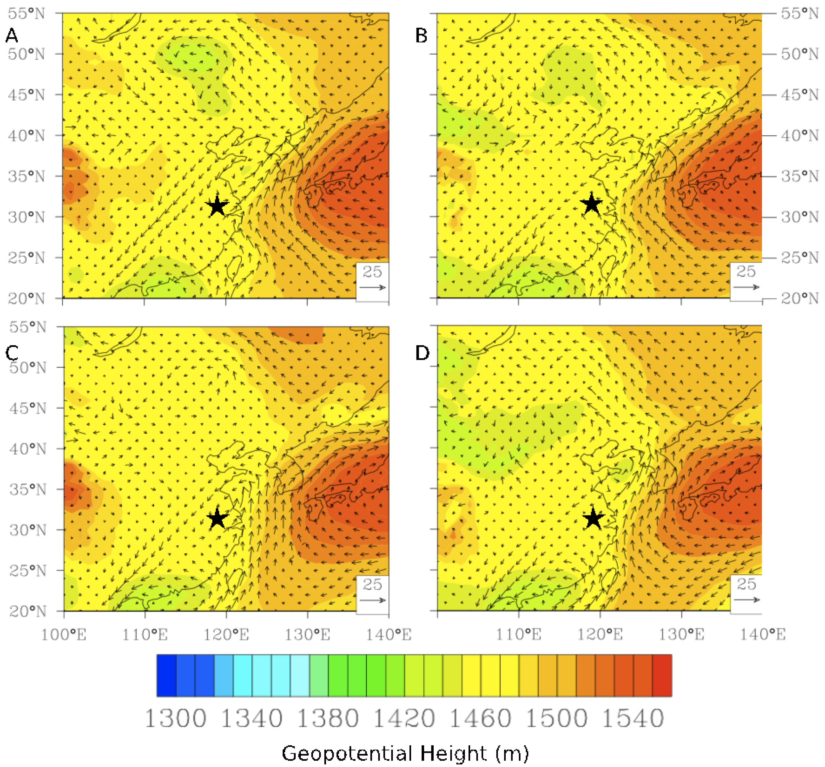
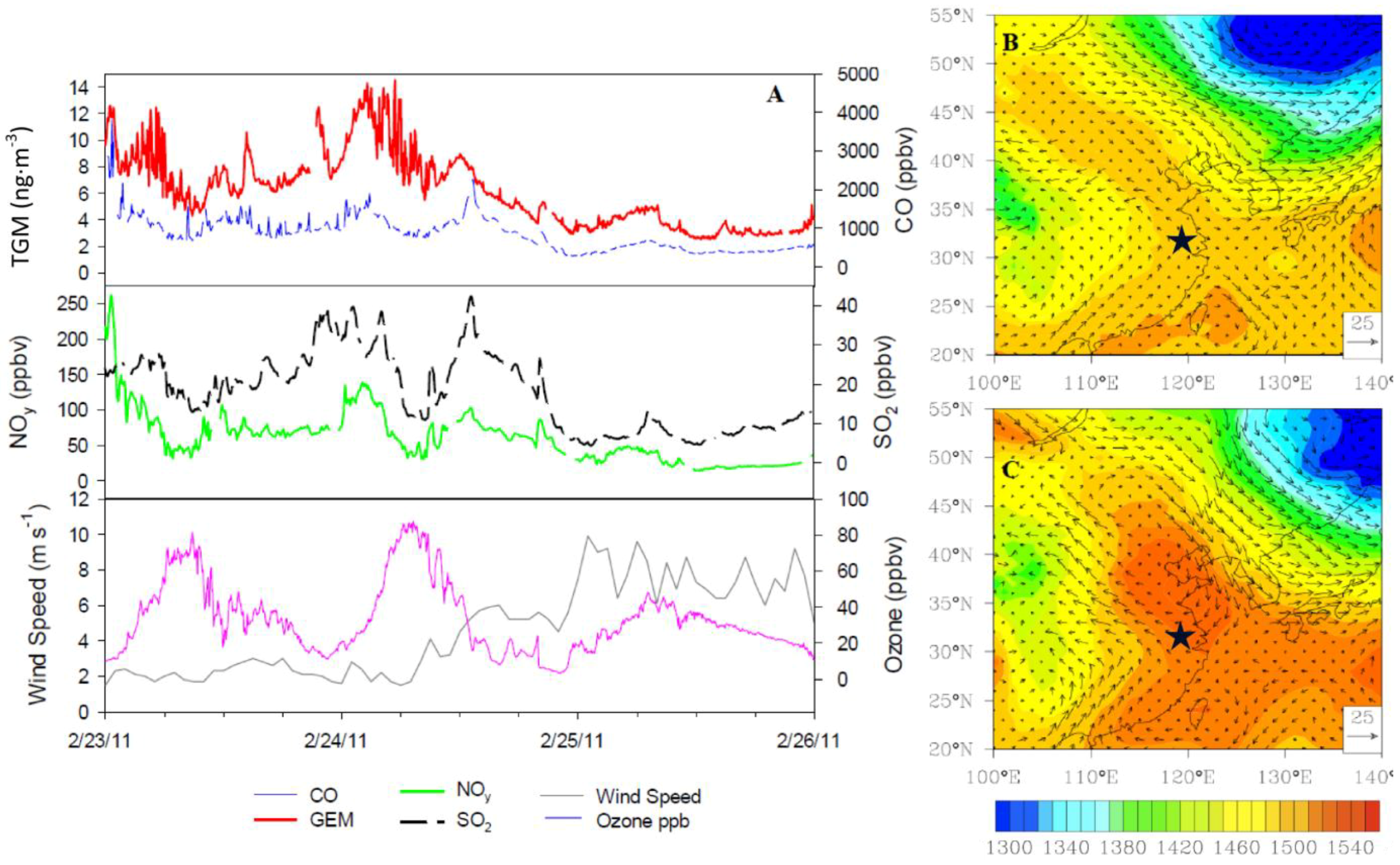
The accumulation of high TGM concentrations in this region started approximately five days earlier on 17 February 2011 (not shown). The TGM concentrations built up in nightly peaks and daytime lows over the course of the preceding week until reaching peak concentrations at approximately 2:30 UT on 24 February 2011. Illustrated in Figure 17, the trace gases CO, SO₂, and NO_y behave similarly to TGM, while O₃ acts differently and peaks in the afternoon as expected. Wind speeds remain low around 2 m∙s⁻¹ allowing emissions to build up locally until approximately 6:00 UT when wind speeds rose and all pollutant concentrations fell due to ventilation. Furthermore there is a stationary front observed at the 850 hPa level on the 24 February 2011causing the stagnant conditions to evolve to increased winds, which finally ventilated the region (Figure 17B,C).

The episodes have differing behavior in terms of correlation of TGM with different trace gases (Table 1). Generally if one trace gas was correlated with TGM, then all trace gases were. The defining characteristic of these episodes was the low wind speeds indicative of YRD sources. Although the sources were within the YRD, fingerprinting individual point sources of pollution proved intractable due to the density and diversity of source types within the YRD.

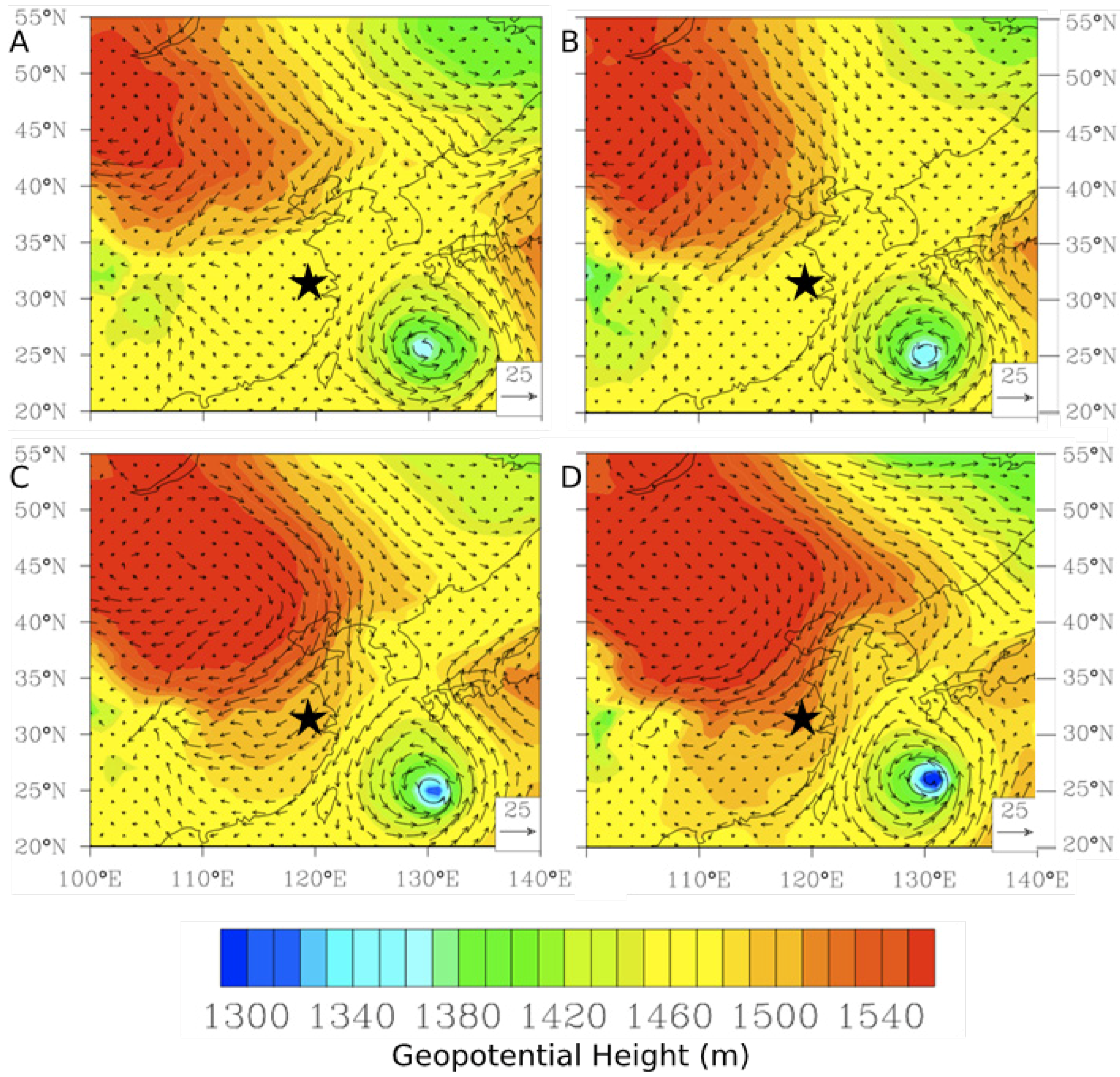
Figure 17. Evolution of an episode of high TGM on 24 February 2011 (A) Time series of five-min average concentrations of trace gases and hourly wind speed. (B) Geopotential height at the 850 hPa level along with wind vectors at 6:00 UT on 24 February 2011. (C) Geopotential height at the 850 hPa level along with wind vectors at 0:00 UT on 25 February 2011. The star ( ) indicates the location of Nanjing.

Figure 17. Evolution of an episode of high TGM on 24 February 2011 (A) Time series of five-min average concentrations of trace gases and hourly wind speed. (B) Geopotential height at the 850 hPa level along with wind vectors at 6:00 UT on 24 February 2011. (C) Geopotential height at the 850 hPa level along with wind vectors at 0:00 UT on 25 February 2011. The star ( ) indicates the location of Nanjing.

3. Experimental Methods

3.1. Site Description and Data Collection

Measurements were made atop a dormitory on the campus of Nanjing University in central Nanjing, China surrounded by heavily used roadways in a dense urban area with a population exceeding 8 million, see Zhu et al. for a map of the location and nearby sources [9]. The inlet height was approximately 70m above ground level. Total gaseous mercury was sampled using a Tekran 2537B mercury vapor analyzer. The Tekran analyzer sampled at a rate of 1 standard L min⁻¹ through PFA tubing. This instrument uses gold amalgamation of TGM in two separate cartridges sampled over 5 minute intervals. The mercury is then desorbed and detected using atomic fluorescence. The detection limit for the instrument was ~0.1 ng∙m⁻³, which over a 5 minute sampling interval equates to 0.5 pg of Hg. Automatic calibration of the instrument was performed using the internal mercury permeation source set to 114.4 pg every 24 hours. The quality control (QC) protocols were based on recommendations in Steffen et al. [40]. The QC protocols were adjusted to deal with the sampling TGM, rather than speciatated mercury. Data was checked to make sure cartridges A and B were within 5% of one another over the entire sampling interval. When data containing∙multiple peaks during desorption, baseline voltage deviations >0.1, baseline voltage shifts of greater than 0.01 V, and sampling volume more than ± 5% from expected the data was rejected and not used in the data set. All data after 31 October 2011, was rejected due to high baseline deviation and multiple peak detection, leaving too few data points for meaningful analysis. Further information about the operation of the 2537B can be found in Zhu et al. [9] and Mao et al. [37].

Concurrent measurements of carbon monoxide (CO), carbon dioxide (CO₂), sulfur dioxide (SO₂), water vapor (H₂O), and reactive nitrogen (NO_y) were conducted. Carbon monoxide was measured using a Thermo model 48i-TLE gas correlation filter instrument and operated according to Mao and Talbot [41]. Measurements of carbon dioxide and water vapor were made using a Li-Cor Li-7000 differential non-dispersive infrared analyzer operated in keeping with Talbot et al. [42]. Sulfur dioxide measurements were made using the Teledyne-API 100E UV fluorescence analyzer and measurements of NO/NOy were made using the Teledyne-API 200EU by chemiluminescence and both were operated conforming to the procedures in Talbot et al. [42]. Additionally, meteorological data such as ground level wind speed and direction were obtained from the National Meteorological Station of Nanjing (ID 58238, 31.9°N, 118.9°E) on an hourly basis, which is not collocated with the Nanjing University site.

Synoptic scale meteorology was studied using several different tools. National Oceanic and Atmospheric Administration (NOAA) Hybrid Single Particle Lagrangian Integrated Trajectory (HYSPLIT) model plots were used to identify air mass movements and potential source regions. The model runs were all performed over five days using the NOAA Global Data Assimilation System (GDAS) data set for dates of interest with a 3 hour and 1° × 1° time and spatial resolution respectively. Furthermore, geopotential height and wind vectors from National Center for Atmospheric Research and National Centers for Environmental Prediction (NCAR/NCEP) reanalysis data (http://www.esrl.noaa.gov/psd/data/composites/day/) were used to investigate the evolution of dynamic systems during∙mercury episodes of interest.

3.2. Lagrangian Dispersion Modeling

Lagrangian particle dispersion modeling (LPDM) simulations of mercury were carried out for selected episodes during the measurement period to estimate TGM concentrations determined by the anthropogenic sources that are documented in the existing emission inventory. The simulation method was developed and evaluated by Ding et al. [43] using the HYSPLIT model [44]. For each sample, 3,000 particles were released from the altitude of 100 m over the measurement site and were traced backward for a 20-day period. The “footprint” residence time (i.e., retroplumes) of each sample was calculated and multiplied by emission to estimate potential source contributions to mercury mixing ratio [43]. The 1.25° × 1.25° Japanese Reanalysis Project reanalysis (JRA) data from the Japan Meteorological Agency was used to drive the Lagrangian dispersion model. The mercury mixing ratios were calculated for every 3 hour during the selected episode based on the calculated retroplumes and AMAP mercury emission inventory [4], a global emission data for the year 2010 with a resolution of 0.5° × 0.5°.

4. Conclusions

Ten months of TGM data was analyzed to understand mercury dynamics in Nanjing, China. The background concentration of TGM was found to be 2.2 ng∙m⁻³. Periods of background concentrations of TGM were investigated and the free troposphere was found to be the source region. Air masses from the free troposphere arriving in Nanjing contained TGM concentrations from greatest to least over the South China Sea, Central Asia, and the Arctic. These findings indicate a possible heterogeneity of TGM in the free troposphere in addition to conceivable transport from Europe and the South China Sea to East Asia. The unusual diel pattern of TGM does not indicate volatilization as the dominant source in summer, accounting for approximately 16% increase in TGM. Furthermore, the correlation of TGM with SO₂ indicates an underestimation of anthropogenic emissions in present inventories. Moreover underrepresented YRD sources were observed with the arrival of TGM transported from other areas most notably Shandong and Hebei provinces.

Nanjing experienced extraordinarily high episodes of TGM concentrations over the study period. The causes of the explosive mercury concentrations appear to be multi-faceted. The episodes had three identified causes: YRD emission buildup, Transport, and the summer monsoon. So few episodes of each type were identified due the complexity of the system this work was conducted in and therefore only on occasion did one factor dominate enough for identification. The buildup of YRD emissions made up the greatest number of episodes (50%) and occurred in tandem with low winds and accumulation of other trace gases. The transport of TGM came from rural regions of Shandong and Hebei provinces, the largest areas of ASGM in China, indicating that currently undocumented and/or illegal ASGM could be an important source to TGM to the YRD. The TGM episodes linked to the summer monsoon appear to be a synergistic interaction of mercury transport from the southwest, where the largest proportion of mercury is emitted in China, inversions caused by agricultural biomass burning, and to a small extent revolatilization [9]. It appears that TGM emissions are underestimated for China and especially the YRD. These emissions have the potential to be transported to sensitive oceanic ecosystems as well as interhemispherically affecting the global atmosphere.

References and Notes

1. Schroeder, W.H.; Munthe, J. Atmospheric mercury—An overview. Atmos. Environ. 1998, 32, 809–822. [Google Scholar] [CrossRef]
2. Amos, H.M.; Jacob, D.J.; Streets, D.G.; Sunderland, E.M. Legacy impacts of all-time anthropogenic emissions on the global mercury cycle. Glob. Biogeochem. Cycle 2013, 27, 410–421. [Google Scholar] [CrossRef]
3. Selin, N.E. Global biogeochemical cycling of mercury: A review. Annu. Rev. Environ. Resour. 2009, 34, 43–63. [Google Scholar] [CrossRef]
4. AMAP/UNEP. Techincal Background Report for the Global Mercury Assessment 2013; Arctic Monitoringand Assessment Programme, Oslo, Norway/UNEP ChemicalsBranch: Geneva, Switzerland, 2013. [Google Scholar]
5. Pacyna, E.G.; Pacyna, J.M.; Sundseth, K.; Munthe, J.; Kindbom, K.; Wilson, S.; Steenhuisen, F.; Maxson, P. Global emission of mercury to the atmosphere from anthropogenic sources in 2005 and projections to 2020. Atmos. Environ. 2010, 44, 2487–2499. [Google Scholar] [CrossRef]
6. Fu, X.; Feng, X.; Sommar, J.; Wang, S. A review of studies on atmospheric mercury in China. Sci. Total Environ. 2012, 421–422, 73–81. [Google Scholar] [CrossRef]
7. Pan, L.; Lin, C.-J.; Carmichael, G.R.; Streets, D.G.; Tang, Y.; Woo, J.-H.; Shetty, S.K.; Chu, H.-W.; Ho, T.C.; Friedli, H.R.; et al. Study of atmospheric mercury budget in East Asia using STEM-Hg∙modeling system. Sci. Total Environ. 2010, 408, 3277–3291. [Google Scholar]
8. Streets, D.G.; Hao, J.; Wu, Y.; Jiang, J.; Chan, M.; Tian, H.; Feng, X. Anthropogenic mercury emissions in China. Atmos. Environ. 2005, 39, 7789–7806. [Google Scholar] [CrossRef]
9. Zhu, J.; Wang, T.; Talbot, R.; Mao, H.; Hall, C.B.; Yang, X.; Fu, C.; Zhuang, B.; Li, S.; Han, Y.; et al. Characteristics of atmospheric total gaseous mercury (TGM) observed in urban Nanjing, China. Atmos. Chem. Phys. 2012, 12, 12103–12118. [Google Scholar] [CrossRef]
10. Zhang, L.; Wang, S.X.; Wang, L.; Hao, J.M. Atmospheric mercury concentration and chemical speciation at a rural site in Beijing, China: Implications of mercury emission sources. Atmos. Chem. Phys. 2013, 13, 10505–10516. [Google Scholar] [CrossRef]
11. Lin, C.-J.; Pan, L.; Streets, D.G.; Shetty, S.K.; Jang, C.; Feng, X.; Chu, H.-W.; Ho, T.C. Estimating∙mercury emission outflow from East Asia using CMAQ-Hg. Atmos. Chem. Phys. 2010, 10, 1853–1864. [Google Scholar] [CrossRef]
12. Sheu, G.; Lin, N.; Lee, C.; Wang, J.; Chuang, M.; Wang, S.; Chi, K.H.; Ou-Yang, C. Distribution of atmospheric mercury in northern Southeast Asia and South China Sea during Dongsha Experiment. Atmos. Environ. 2013, 78, 174–183. [Google Scholar] [CrossRef]
13. Ci, Z.J.; Zhang, X.S.; Wang, Z.W.; Niu, Z.C.; Diao, X.Y.; Wang, S.W. Distribution and air-sea exchange of mercury (Hg) in the Yellow Sea. Atmos. Chem. Phys. 2011, 11, 2881–2892. [Google Scholar] [CrossRef]
14. Shen, L.; Gunson, A.J. The role of artisanal and small-scale mining in China’s economy. J. Clean. Prod. 2006, 14, 427–435. [Google Scholar] [CrossRef]
15. Huang, X.; Li, M.; Friedli, H.R.; Song, Y.; Chang, D.; Zhu, L. Mercury emissions from biomass burning in China. Environ. Sci. Technol. 2011, 45, 9442–9448. [Google Scholar] [CrossRef]
16. Yihui, D.; Chan, J.C.L. The East Asian summer monsoon: An overview. Meteorol. Atmos. Phys. 2005, 89, 117–142. [Google Scholar] [CrossRef]
17. Chen, L.; Liu, M.; Xu, Z.; Fan, R.; Tao, J.; Chen, D.; Zhang, D.; Xie, D.; Sun, J. Variation trends and influencing factors of total gaseous mercury in the Pearl River Delta-A highly industrialised region in South China influenced by seasonal monsoons. Atmos. Environ. 2013, 77, 757–766. [Google Scholar] [CrossRef]
18. Ding, A.J.; Fu, C.B.; Yang, X.Q.; Sun, J.N.; Petäjä, T.; Kerminen, V.-M.; Wang, T.; Xie, Y.N.; Herman, E.; Zheng, L.F.; et al. Intense atmospheric pollution modifies weather: A case of mixed biomass burning with fossil fuel combustion pollution in the Eastern China. Atmos. Chem. Phys. Discuss. 2013, 13, 14377–14403. [Google Scholar] [CrossRef]
19. Newell, R.E.; Evans, M.J. Seasonal changes in pollutant transport to the North Pacific: The relative importance of Asian and European sources. Geophys. Res. Lett. 2000, 27, 2509–2512. [Google Scholar] [CrossRef]
20. Jaffe, D.; Prestbo, E.; Swartzendruber, P.; Weiss-Penzias, P.; Kato, S.; Takami, A.; Hatakeyama, S.; Kajii, Y. Export of atmospheric mercury from Asia. Atmos. Environ. 2005, 39, 3029–3038. [Google Scholar] [CrossRef]
21. Sheu, G.-R.; Lin, N.-H.; Wang, J.-L.; Lee, C.-T.; Ou Yang, C.-F.; Wang, S.-H. Temporal distribution and potential sources of atmospheric mercury measured at a high-elevation background station in Taiwan. Atmos. Environ. 2010, 44, 2393–2400. [Google Scholar] [CrossRef]
22. Zhang, F.; Zhou, L.; Conway, T.J.; Tans, P.P.; Wang, Y. Short-term variations of atmospheric CO2 and dominant causes in summer and winter: Analysis of 14-year Continuous observational data at Waliguan, China. Atmos. Environ. 2013, 77, 140–148. [Google Scholar] [CrossRef]
23. Tseng, C.M.; Lamborg, C.H.; Hsu, S.C. A unique seasonal pattern in dissolved elemental mercury in the South China Sea, a tropical and monsoon-dominated marginal sea. Geophys. Res. Lett. 2013, 40, 167–172. [Google Scholar] [CrossRef]
24. Berman, S.; Ku, J.-Y.; Rao, S.T. Spatial and temporal variation in the mixing depth over the northeastern United States during the summer of 1995. J. Appl. Meteorol. 1999, 38, 1661–1673. [Google Scholar] [CrossRef]
25. Chan, L.; Deng, Q.-H.; Liu, W.-W.; Huang, B.-L.; Shi, L.-Z. Characteristics of ventilation coefficient and its impact on urban air pollution. J. Cent. South Univ. Technol. 2012, 19, 615–622. [Google Scholar] [CrossRef]
26. Obrist, D.; Hallar, A.G.; McCubbin, I.; Stephens, B.B.; Rahn, T. Atmospheric mercury concentrations at storm peak laboratory in the Rocky Mountains: Evidence for long-range transport from Asia, boundary layer contributions, and plant mercury uptake. Atmos. Environ. 2008, 42, 7579–7589. [Google Scholar] [CrossRef]
27. Mao, H.; Talbot, R.W.; Sive, B.C.; Youn Kim, S.; Blake, D.R.; Weinheimer, A.J. Arctic mercury depletion and its quantitative link with Halogens. J. Atmos. Chem. 2010, 65, 145–170. [Google Scholar] [CrossRef]
28. Nguyen, H.T.; Kim, K.-H.; Shon, Z.-H.; Hong, S. A review of atmospheric mercury in the polar environment. Crit. Rev. Environ. Sci. Technol. 2009, 39, 552–584. [Google Scholar] [CrossRef]
29. Talbot, R.; Mao, H.; Scheuer, E.; Dibb, J.; Avery, M. Total depletion of Hg° in the upper troposphere-lower stratosphere. Geophys. Res. Lett. 2007. [Google Scholar] [CrossRef]
30. Boudala, F.S.; Folkins, I.; Beauchamp, S.; Tordon, R.; Neima, J.; Johnson, B. Mercury flux measurements over air and water in Kejimkujik National Park, Nova Scotia. Water Air Soil Pollut. 2000, 122, 183–202. [Google Scholar] [CrossRef]
31. Fu, X.; Wang, S.; Zhao, B.; Xing, J.; Cheng, Z.; Liu, H.; Hao, J. Emission inventory of primary pollutants and chemical speciation in 2010 for the Yangtze River Delta Region, China. Atmos. Environ. 2013, 70, 39–50. [Google Scholar] [CrossRef]
32. Vaida, V.; Kjaergaard, H.G.; Hintze, P.E.; Donaldson, D.J. Photolysis of sulfuric acid vapor by visible solar radiation. Science 2003, 299, 1566–1568. [Google Scholar] [CrossRef]
33. Lin, C.-J.; Gustin, M.S.; Singhasuk, P.; Eckley, C.; Miller, M. Empirical Models for Estimating∙mercury Flux from Soils. Environ. Sci. Technol. 2010, 44, 8522–8528. [Google Scholar] [CrossRef]
34. Zhao, D.; Su, B.; Zhao, M. Soil moisture retrieval from satellite images and its application to heavy rainfall simulation in Eastern China. Adv. Atmos. Sci. 2006, 23, 299–316. [Google Scholar] [CrossRef]
35. Sprovieri, F.; Pirrone, N.; Ebinghaus, R.; Kock, H.; Dommergue, A. A review of worldwide atmospheric mercury measurements. Atmos. Chem. Phys. 2010, 10, 8245–8265. [Google Scholar] [CrossRef] [Green Version]
36. Zheng, J.; Ou, J.; Mo, Z.; Yin, S. Mercury emission inventory and its spatial characteristics in the Pearl River Delta region, China. Sci. Total Environ. 2011, 412–413, 214–222. [Google Scholar] [CrossRef]
37. Mao, H.; Talbot, R.; Sigler, J.; Sive, B.; Hegarty, J. Seasonal and diurnal variations of Hg° over New England. Atmos. Chem. Phys. 2008, 8, 1403–1421. [Google Scholar] [CrossRef]
38. Lee, D.S.; Dollard, G.J.; Pepler, S. Gas-phase mercury in the atmosphere of the United Kingdom. Atmos. Environ. 1998, 32, 855–864. [Google Scholar] [CrossRef]
39. Mazur, M.; Mintz, R.; Lapalme, M.; Wiens, B. Ambient air total gaseous mercury concentrations in the vicinity of coal-fired power plants in Alberta, Canada. Sci. Total Environ. 2009, 408, 373–381. [Google Scholar] [CrossRef]
40. Steffen, A.; Scherz, T.; Olson, M.; Gay, D.; Blanchard, P. A comparison of data quality control protocols for atmospheric mercury speciation measurements. J. Environ. Monit. 2012, 14, 752–765. [Google Scholar] [CrossRef]
41. Mao, H.; Talbot, R. O3 and CO in New England: Temporal variations and relationships. J. Geophys. Res.: Atmos. 2004, 109, 1–19. [Google Scholar]
42. Talbot, R.; Mao, H.; Sive, B. Diurnal characteristics of surface level O3 and other important trace gases in New England. J. Geophys. Res.: Atmos. 2005, 110, 1–16. [Google Scholar]
43. Ding, A.; Wang, T.; Fu, C. Transport characteristics and origins of carbon monoxide and ozone in Hong Kong, South China. J. Geophys. Res.: Atmos. 2013, 118, 9475–9488. [Google Scholar]
44. Draxler, R.R.; Hess, G.D. An overview of the HYSPLIT_4 modelling system for trajectories, disterpsion and deposition. Aust. Meteorol. Mag. 1998, 47, 295–308. [Google Scholar]