Article

Water Vapor, Temperature and Wind Profiles within Maize Canopy under in-Field Rainwater Harvesting with Wide and Narrow Runoff Strips

1
Department of Soil, Crop and Climate Sciences, University of the Free State, P.O. Box 339, Bloemfontein 9300, South Africa
2
Crops for the Future Research Centre, The University of Nottingham Malaysia Campus, Jalan Broga, 43500 Semenyih, Malaysia
3
School of Environmental Science, Faculty of Science and Agriculture, University of KwaZulu-Natal, Pietermaritzburg 3201, South Africa
*
Author to whom correspondence should be addressed.
Atmosphere 2013, 4(4), 428-444; https://doi.org/10.3390/atmos4040428
Submission received: 7 October 2013 / Revised: 6 November 2013 / Accepted: 13 November 2013 / Published: 29 November 2013
(This article belongs to the Special Issue Agrometeorology: From Scientific Analysis to Operational Application)

Abstract

:
Micrometeorological measurements were used to evaluate heat and water vapor to describe the transpiration (Ev) and soil evaporation (Es) processes for wide and narrow runoff strips under in-field rainwater harvesting (IRWH) system. The resulting sigmoid-shaped water vapor (ea) in wide and narrow runoff strips varied in lower and upper parts of the maize canopy. In wide runoff strips, lapse conditions of ea extended from lowest measurement level (LP) to the upper middle section (MU) and inversion was apparent at the top of the canopy. The virtual potential temperature (θv) profile showed no difference in middle section, but the lower and upper portion (UP) had lower θν in narrow, compared to wide, strips, and LP-UP changes of 0.6 K and 1.2 K were observed, respectively. The Ev and Es within the canopy increased the ea concentration as determined by the wind order of magnitude. The ea concentration reached peak at about 1.6 kPa at a range of wind speed value of 1.4–1.8 m∙s−1 and 2.0–2.4 m∙s−1 for wide and narrow treatments, respectively. The sparse maize canopy of the wide strips could supply more drying power of the air in response to atmospheric evaporative demand compared to narrow strips. This is due to the variation in air flow in wide and narrow runoff strips that change gradients in ea for evapotranspiration processes.

1. Introduction

The growing interest in the application of the integrated studies of plant water use and micrometeorological parameters for alternative evaluations is a noteworthy experience in tillage management. Profiles of water vapor pressure (ea), virtual potential temperatures (θν), and wind speed (u) are three vital measurements in micrometeorological studies within crop canopies. Basic understanding of the micrometeorological variable profiles and their relationships within the canopy surface is an essential step to quantify and evaluate the heat and water vapor exchange processes between the atmosphere and canopy. Conservation tillage techniques, such as alternate basin and runoff area of in-field rainwater harvesting systems (IRWH) affect the momentum and heat transfer inside the canopy. The IRWH system is a different approach to dry land farming, and as its focus is water use, the different part of the Soil-Plant-Atmosphere water continuum (SPAC) are all an integral part of the system [1]. Much research has been done on the soil and crop parameters within IRWH [2,3]. However, little effort has been invested in characterizing the atmospheric components of this soil-plant-atmosphere system [4]. Although many studies have measured the soil water balance as a source of water for the IRWH crop production, no attempt has been made to quantify the demand side of the equation from an atmospheric point of view. The wider adoption of IRWH has increased the research interest in IRWH and posed a number of questions about the least understood parts of the system, namely the micrometeorological processes and parameters.
Verification and characterization of profile relationships is the first important step to obtaining reliable flux estimations [5]. In a cropped field, the height where the heat energy exchange occurs depends on the profiles of dynamic micrometeorological parameters and on the flow within the thermal internal boundary layer [6]. These processes are used, not only to aid the understanding of turbulent transport, but also as a tool that allows the vertical turbulent fluxes to be predicted from the more-easily measured and predicted vertical gradients of the profiles. In this regard, measurements of micrometeorological parameters (such as ea, θν, and u) at different levels and during different crop growth stages contribute to the understanding of how the net radiation in a crop field is balanced by the combination of sensible and latent heat fluxes, and the conduction of heat flux through soil surface, as well as heat storage [7]. However, progress in understanding micrometeorological variable profile relationships requires intensive and continuous micrometeorological measurements [8], with adequate attention given to high accuracy and reliability [9]. According to Monteith and Unsworth [9], with sufficiently precise instrumentation, profiles of ea, θν, and u can be measured to represent some vertical gradients within a crop canopy. Therefore, the use of flux-profile relationships is central to many micrometeorological boundary-layer studies [10]. The understanding of the profile relationships of micrometeorological variables together with flux estimation is an essential step in matching the rainwater supply to the soil with the demand by the atmosphere, thereby improving productivity and sustainability in any water conservation agricultural technique [11,12]. Characterization of ea, θν, and u profiles within a maize canopy, over an alternative arrangement of basin and runoff areas, is of paramount importance in evaluating the heat exchange, and hence the available energy for evapotranspiration and, ultimately, available water for crop production.
In this study therefore, vertical profiles of micrometeorological variables at different maize growth stages were assessed, while making certain assumptions of horizontal heterogeneity of air temperature and water vapor and the wind speed drivers across the experimental field. From the measurements of ea, θν, and u, simple profile relationships were derived that were then used to evaluate the heat and water vapor parameters. These heat and water vapor parameters were used to estimate transpiration and soil water evaporation for wide and narrow strips under the IRWH system. The aims of this study, therefore, were to evaluate the impact of different water harvesting practices on the vertical profiles of ea, θν, and u, by comparing wide and narrow runoff strip lengths (RSL) during different growth stages andto describe relationships between the u versus ea profiles within a maize canopy.

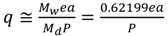
2. Theoretical Basis and Description of Methods

Using micrometeorological measurements within a maize canopy, simple thermodynamic relations were adopted, to understand the flow of heat and water vapor processes, as follows. In thermodynamics, the density of air and total atmospheric pressure depend mainly on the effects of altitude, air temperature, and water vapor pressure. For moist unsaturated air, with Dalton’s law of partial pressure (P = Pd + ea), where P is the atmospheric pressure (Pa), Pd is pressure of dry air, one can apply a temperature dependent function to the specific gas constant for dry air, instead of humidity-dependent variables. Then, in practice, the correction is adapted to the temperature by using the θν as a parameter for heat exchange processes. According to Stull [13], the virtual temperatures are defined as the temperatures that dry air would have if its pressure and density were equal to that of moist air. To account for the effect of moisture on buoyancy force a θν is defined as:
θν = θ(1 + 0.61q)
where the specific humidity is denoted by q and θν is the virtual potential temperature and is always greater than actual temperature and the difference between the two may be as large as 7 K in warm tropical areas and be as small as 2 K in mid-latitude areas [8]. Therefore, when buoyancy forces are involved, gradients of θν are preferable, rather than considering the actual potential temperatures (θ) [6,8,14,15].
Different studies express the water vapor in the air using different terms [8,16]. The parameter most often used in micrometeorology studies is the specific humidity (q):
Atmosphere 04 00428 i001
where Mw and Md are molecular mass of water and dry air, is directly related to the ea, which is a the partial pressure exerted by the water vapor in the boundary layer.
According to Savage et al. [12], Malek [17], and Arya [18], ea variables are preferred in comparing and calculating variation in water vapor instead of relative humidity, which is temperature dependent. Water vapor has dominant effect on the radiative heating that leads to release of latent heat and fundamental driver of atmospheric demand. As parameters for expressing humidity and temperature are interconnected, they must be manipulated to calculate the required derived variables. Relative humidity, RH (%) is defined as:
RH = 100 × (ea/es)
where es is saturated vapor pressure (KPa), calculated using the following equation:
es = 0.6108exp (17.2694T/(273.3 + T))
where T is the temperature (°C), then ea was calculated using es and RH, and was used to express moisture profiles in kPa.
The “temperature dependent constant”, affects the value of calculated heat energy flux densities and, hence, a full understanding of the variation of the psychrometric constant, γ (kPa∙K−1) is important. It is also expected that the removal of water vapor or evaporation from a surface is dependent on the atmospheric pressure. Therefore, the correction of the psychrometric constant for a given atmospheric pressure other than sea level pressure is imperative. The common relationship is given as γ = γo(P/Po) [6,12], where γ is the psychrometric constant at atmospheric pressure, P and γo is psychrometric constant at sea level pressure (Po = 101.325 kPa). This leads to the appropriate interpretation of heat and mass transfer processes within a crop canopy. In the profile analysis, θν and ea were calculated using the above procedure, as follows. The γ for this altitude (h = 1,354 m) was calculated as 0.055 KPa∙K−1, assuming that the density of the air, ρ is 1.211 kg∙m−3, and the atmospheric pressure, P = 85.245 kPa was computed by using an equation, p = p0 - ρgh.

3. Materials and Methods

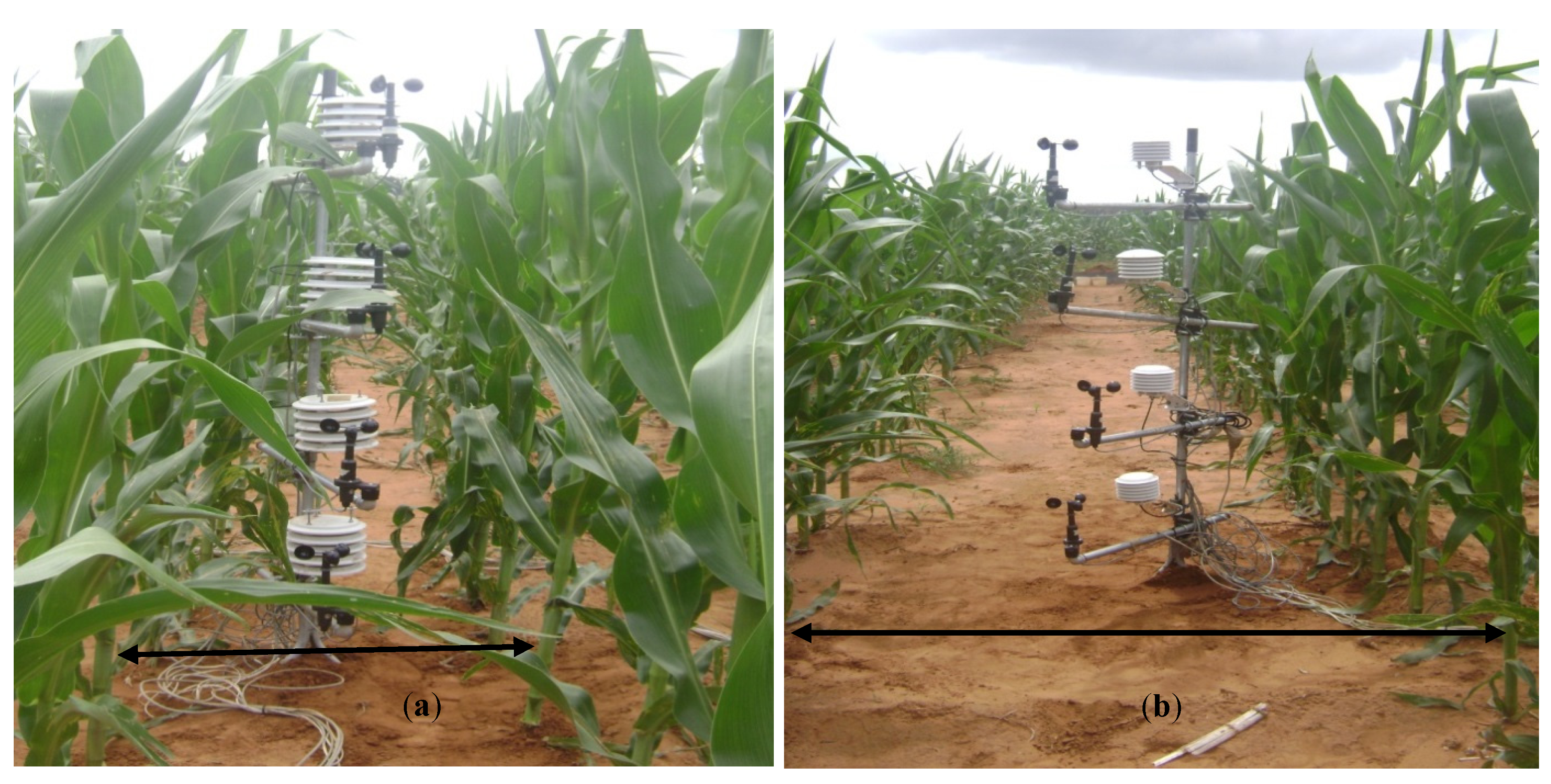
3.1. Experimental Design and Layout
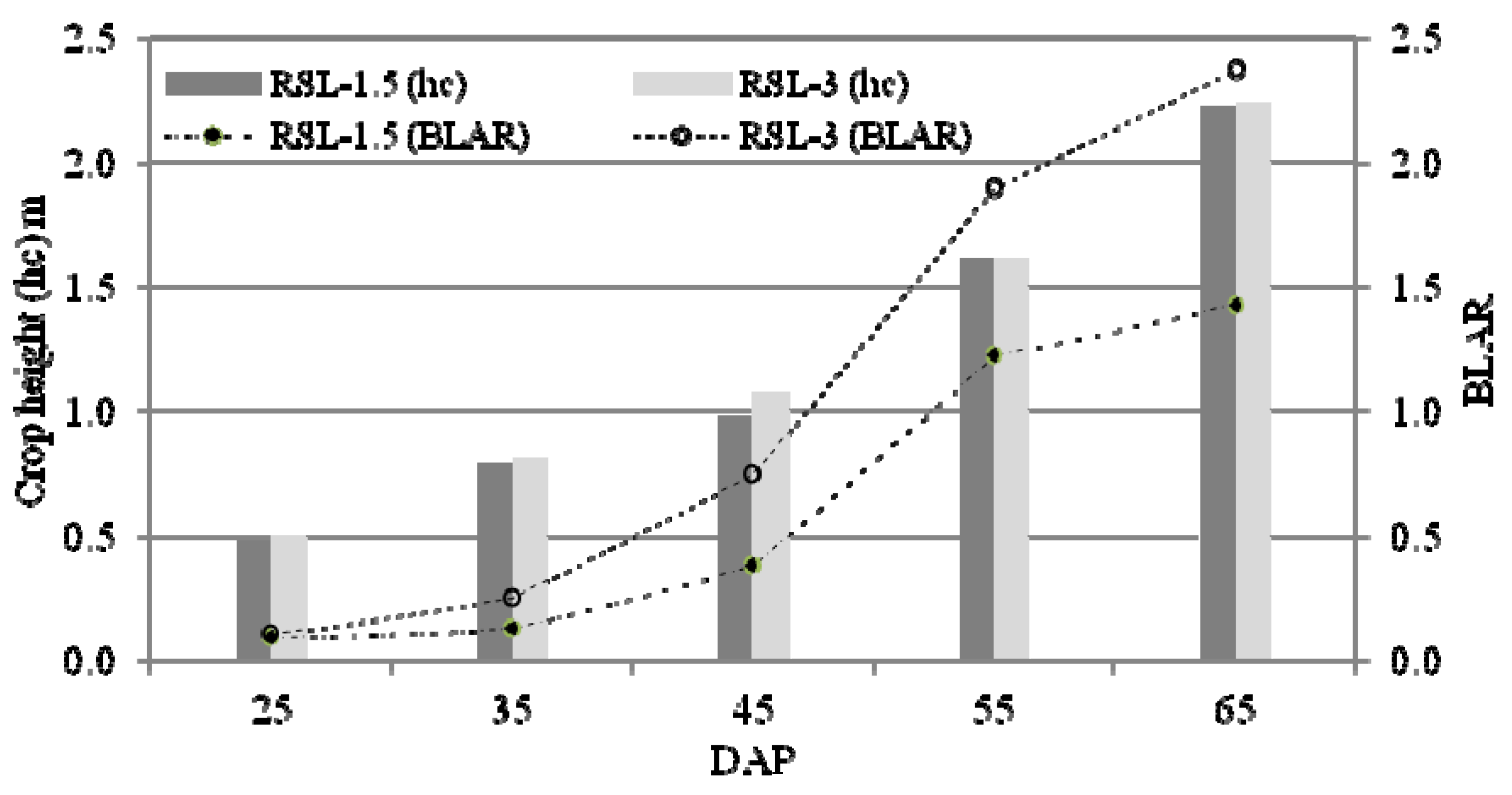
A field experiment with maize under IRWH was conducted during the September 2008 growing season at the Kenilworth Experimental Farm (Latitude 29°01'S, Longitude 2°09'E, Altitude 1,354 m above sea level) of the University of the Free State near Bloemfontein in the Free State, South Africa. The 1 ha maize field under IRWH was designed with each main plot consisting of four IRWH runoff strip length (RSL) treatments, with rows extending the entire length of the field in the East-West (E-W) direction. In this study, two RSL treatments were selected, viz. 3 m and 1.5 m representations for a wide and a narrow RSL, respectively. During the maize growing season, profiles of temperature, humidity, and wind speed measurements were continually performed within the maize canopy. During the measurement period, three consecutive growth stages with specific runs of measurement periods were selected. Early and late vegetative growth stages were represented after the crop canopy has attained a height of 1.2 m and 1.6 m, and at maximum canopy height (average of 2.2 m) when the crop was in the reproductive stage.
Micrometeorological profile measurements were made at four levels above the soil surface and the sensors were installed at various heights by shifting them on vertical poles, according to the crop growth. The heights were changed three times through the growing period, as indicted in Table 1. The focus of the analysis was on the vertical profiles of the ea, θν, and u, in both wide (3 m) and narrow (1.5 m) runoff strips. When the crop attained a height of 1.2 m and later 1.6 m, the set-up of the instruments were fixed above the soil surface within the canopy at the four described levels of 0.3, 0.6, 0.9, and 1.2 m and 0.4, 0.8, 1.2, and 1.6 m, respectively. When crop height was at a maximum (2.2 m), at reproductive stage, the sensors were moved up to levels of 0.55, 1.10, 1.65, and 2.2 m (Table 1).
Table 1. Micrometeorology measurement days and sensor position (zi) at heights above ground surface levels of the micrometeorology measurements.
Growth StagesEarly VegetativeLate VegetativeMaximum Height
Observed Period (Date)5–11 February 200920–25 February 200910–15 March 2009
DOY *36–4251–5669–74
Profile Position z1 (m)0.300.400.55
Profile Position z2 (m)0.600.801.10
Profile Position z3 (m)0.901.201.65
Profile Position z4 (m) = hc **1.201.602.20
DOY * represents day of year; hc ** is crop height.
In these canopy profile observations, the four layers of measurements were denoted as: upper portion (UP), mid-upper (MU), mid-lower (ML), and lower portion (LP). These portions or layers of the maize canopy represented the top canopy layer, upper part above the midpoint, lower part below the midpoint, and the bottom layer, respectively. The variation in measurement, in these strata (layers) of the vertical profiles, was used to characterize the micrometeorological parameters and their interactions within crop canopies.

3.2. Measurements

In order to measure the profiles within a maize canopy, a tripod stand-pole with extended arms was erected in both wide (RSL-3) and narrow (RSL-1.5) runoff section areas. An identically instrumented tripod was placed in the centre of a runoff section of each treatment by selecting the third runoff strip on the southern side from the four consecutive runoff strips making up each treatment plot (Figure 1). To ensure that the measurements made by different sensors were at the same height in narrow and wide runoff strips, the tripod poles and arms were checked frequently. Care was also taken not to allow the sensors to touch plant parts, in particular in narrow RSL. The position of the sensors was upwind of the vertical pole holding them (prevailing N-NW wind direction). The maize was planted in tramlines on either side of the basin in an E–W direction, 1.1 m apart, at a plant population of 18,000 ha1 in both RSL treatments. The plant spacing within the row was 0.44 and 0.28 m in wide and narrow runoff strips, respectively, to obtain the target plant population across the whole area. Plant samples were taken at 10-day intervals from 15 January to 25 March 2009, at 25, 35, 45, 55, and 65 days after planting (DAP) to monitor the basin leaf area ratio (BLAR), and plant height. The BLAR, expressed as the leaf area measured divided by the basin area, gave values of 2.43 and 1.42 in the wide and narrow RSL treatments at full canopy cover, respectively. This meant that the leaf area was calculated from the same unit area for both RSL treatments. The maximum maize height was 2.2 m.
Figure 1. Sensor arrangements in the runoff section within the maize canopy at 1.6 m crop height on 25 February 2009, for the 1.5 m and 3.0 m length runoff strip. (a) 1.5 m (Narrow RSL); (b) 3.0 m (Wide RSL).
Atmosphere 04 00428 g001

3.3. Instrumentation

Measurements were performed at four levels within the maize canopy: (a) Wind speed was measured using three-cup wheel Sentry anemometers (Model 03001, RM Young, Traverse City, MI, USA) with stalling speed of about 0.15 m∙s−1; and (b) temperature and humidity were monitored using HMP50 temperature and relative humidity probes (Campbell Scientific Inc., Logan, UT, USA) [19], which contained platinum resistance temperature detectors (PRT) and Vaisala-INTERCAP sensors for temperature and relative humidity, respectively. The HMP50 sensors were housed inside white six-plate radiation shields (41303-5A Model) (Figure 1). The position of the sensors within the crop canopy at the four levels is illustrated in Figure 1 for the 1.6 m crop height. All micrometeorological data were recorded on a CR1000X data logger (Campbell Scientific, Logan, UT, USA) [19], every scan was taken every 5 min and averaged over one hour. Instrumentation was frequently checked and data regularly downloaded. Leaf area was measured using leaf area meter (Licor, Model LI-3100 Area Meter, LI-COR Inc. Lincoln, Nebraska, USA).

3.4. Method of Statistical Analysis

To compare the differences in the observations between the two groups, wide and narrow RSLs, for each layer in the profile, a statistical data analysis was conducted using a two-tail paired t-test procedure with SAS 9.1.3 statistical software for Windows (SAS Inst. Inc., 2006) [20]. Significance levels of P ≤ 0.05 and P ≤ 0.01 were used based on the variability associated with the measurements. These comparisons were carried out for three different periods during the season. In addition to statistical methods, graphical and tabular representations were used to illustrate and compare the diurnal variations of the profiles within the canopy for specific days and hours. As most evaporation took place during the daylight hours, the relationships of u and ea were expressed using empirical regression procedures for daytime hours (08:00–17:00) only.

4. Results and Discussion

4.1. Maize Canopy Structure

During the selected vegetative and reproductive periods, the maize crop was growing rapidly (Figure 2). The wide and narrow treatments followed the same trend for both crop height and BLAR, but the wide runoff treatment showed a higher BLAR. In both RSL treatments, the BLAR increased with the plant growth during 35–55 DAP and reached a plateau after 65 DAP (Figure 2). At later growth stages, a significant difference was found for BLAR between wide and narrow runoffs treatments. However, the statistical analysis of the plant height data revealed no significant differences between treatments. The vegetation characteristics of plant density and BLAR have an effect on the processes of heat and water vapor within the maize canopy at different growth stages. The variation in canopy structure of a maize crop under IRWH will be an important consideration when evaluating the vertical distribution of meteorological variables, such as ea, θν, and u, and their role in the energy balance of the canopy and soil surface.
Figure 2. The changes in crop height (hc) and basin leaf area ratio (BLAR) during vegetative and reproductive stages at 10-day intervals from mid-January to March, 2009.
Atmosphere 04 00428 g002

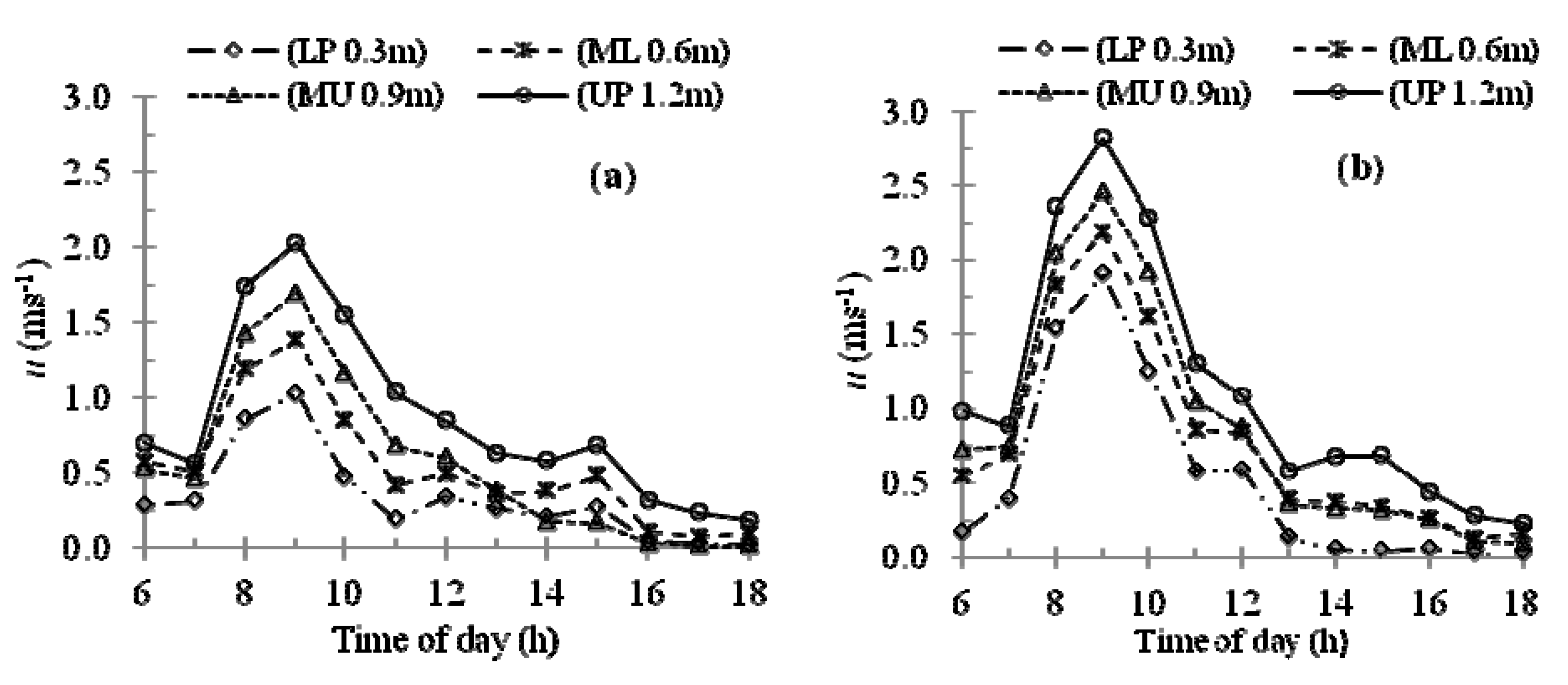
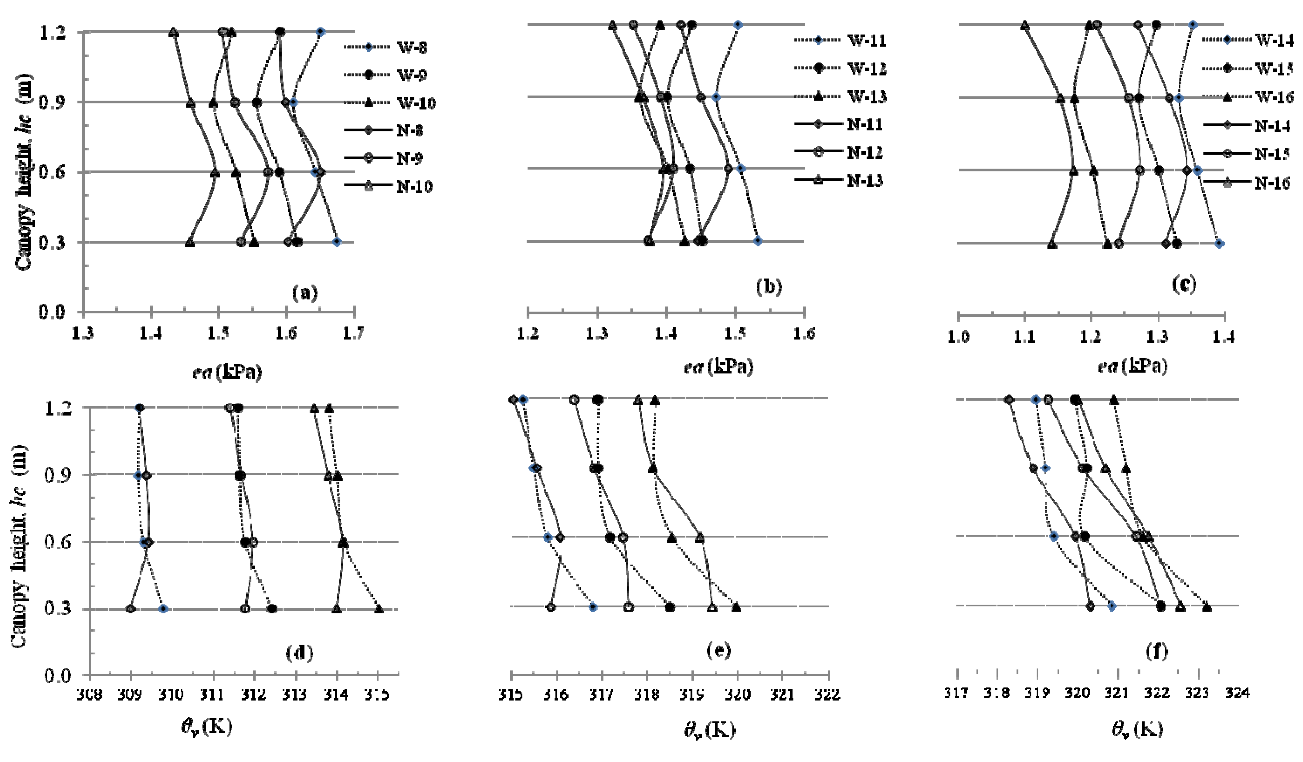
4.2. Comparison of Profiles within the Canopy

During the early vegetative growth stage, both θν and ea had highly significant differences in the UP and LP of the canopy (Table 2). In contrast to the early vegetative stage (hc = 1.2 m), crops at the late vegetative stage (hc = 1.6 m) showed significant differences in all the measured variables (u, θν, and ea) between wide and narrow runoff treatments. In particular, u and ea showed highly significant differences (P < 0.01) at all sampling levels (Table 2). This exhibits the differences of ea concentration delivered to the atmosphere via evaporation that represents available energy within the canopy that can be driven by different wind speed magnitudes. When maximum plant height (average of 2.2 m) was reached, after 65 DAP, highly significant differences for u and ea between the wide and narrow runoff strips were recorded (Table 2). This was in agreement with results obtained for all the profile-levels during the late vegetative stage. However, the θν below the middle of the canopy height was not significantly different, even at P < 0.05, between wide and narrow runoff, while the upper two levels were significant at P < 0.05. The reason for the less or non-significant differences of θν in the lower portion was probably due to very low frequency of measurements. In addition, it would be also apparent to detect, more clearly, all eddies and turbulences close to the soil surface by using fine wire thermocouples. Nevertheless, with little turbulence under low wind conditions (<1 ms−1), almost all the heat exchange between the leaves and air above occurred in the top half of the canopy. The bottom half of the canopy was a very weak heat sink in both wide and narrow runoff strips due to fewer leaves.
Table 2. Statistical comparison between wide and narrow runoff strip length (RSL) treatments for hourly wind speed (u), virtual potential temperature (θν), and actual water vapor pressure (ea).
ParametersLayerEarly Vegetative Stage
(hc = 1.2 m), n = 144
Late Vegetative Stage
(hc = 1.6 m), n = 96
Maximum Crop Height
(hc = 2.2 m), n = 120
Height (m)SignificanceHeight (m)SignificanceHeight (m)Significance
Wind speed
(u)
LP0.30*0.40**0.55**
ML0.60ns0.80**1.10**
MU0.90**1.20**1.65**
UP1.20ns1.60**2.20**
Virtual potential temperature
(θν)
LP0.30**0.40*0.55ns
ML0.60**0.80*1.10ns
MU0.90ns1.20*1.65*
UP1.20**1.60**2.20*
Water vapor pressure
(ea)
LP0.30**0.40**0.55**
ML0.60ns0.80**1.10**
MU0.90ns1.20**1.65**
UP1.20**1.60**2.20**
hc: crop height at top level; LP: lower portion; ML: mid-lower portion; MU: mid-upper portion; UP: upper portion; * P < 0.05; ** P < 0.01; ns = not significant.

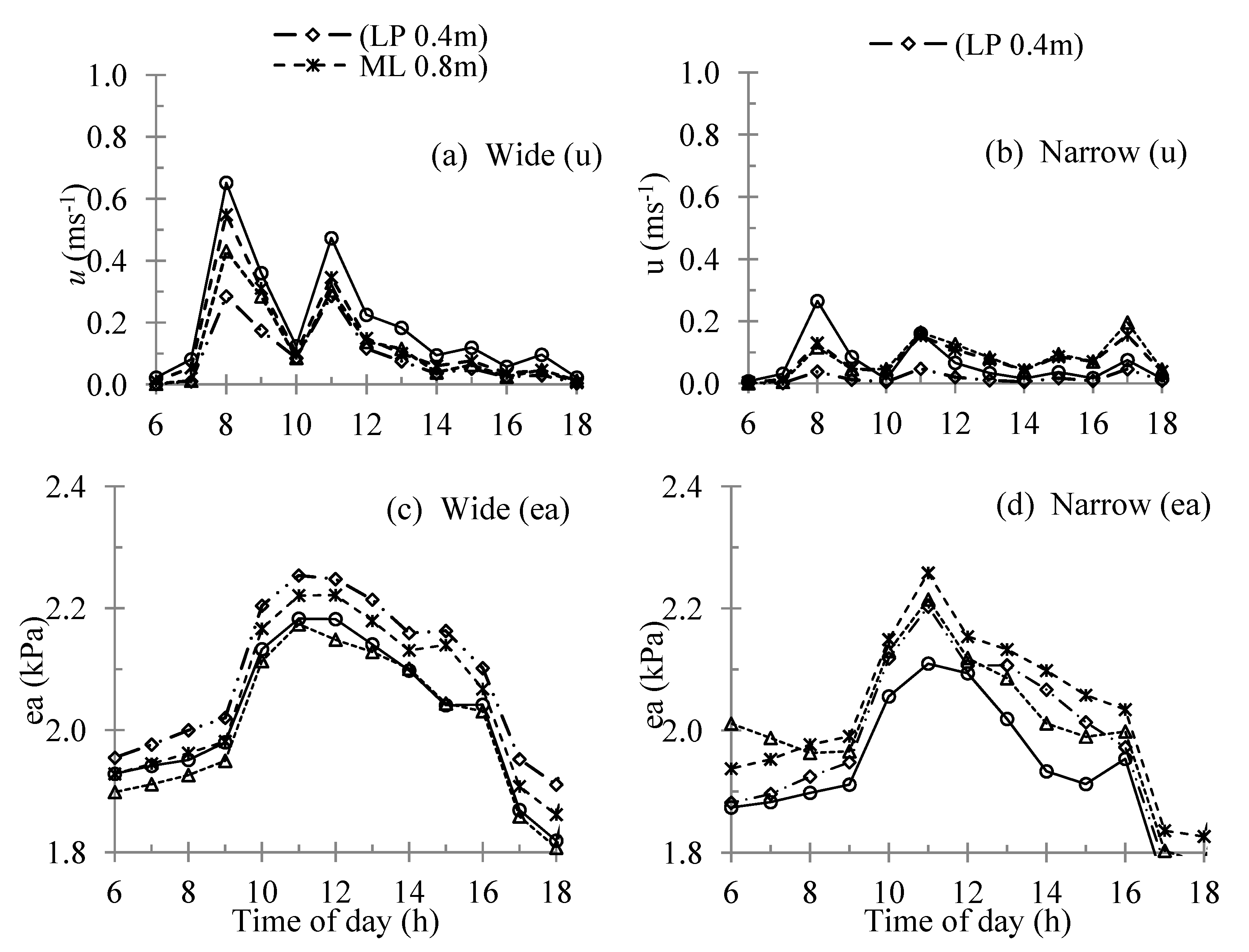
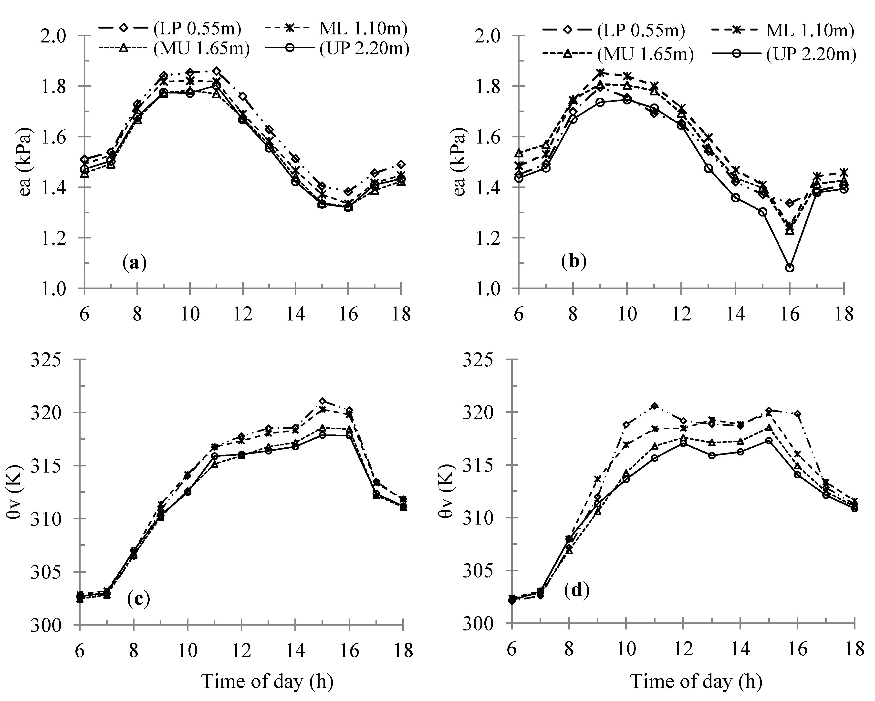
4.3. Diurnal Changes in Profile

4.3.1. Early Vegetative Growth Stage

During the morning, the wind speed in narrow runoff (Figure 3a) was much higher than in wide runoff strips (Figure 3b) at all heights and times. However, as the wind speed decreased on both RSL, by midday (11:00–13:00), the differences became insignificant at 13:00. The hourly profiles of ea in the morning (Figure 4a) and around midday (Figure 4b) both showed sigmoid-shaped ea profiles, with similar LP and UP values. In the wide RSL, for ML, and MU parts of the canopy, the profile of eadecreased slightly (lapse) with height and returned to a higher value in the UP of the canopy (Figure 4), because of the higher wind speed in this part of the canopy (UP). In narrow RSL, the decrease was from ML to UP, near the top of canopy with peak ea in the ML part of canopy. At this stage of vegetative growth, in both wide and narrow runoff sections the moisture concentration in the UP layer decreased as the day progressed with increasing air temperature and the resulting increases in evaporative demand. In the MU portion of the canopy, the ea values decreased with height in both wide and narrow RSLs (Figure 4a). The values of ea decreased throughout the day at each different profile height in both the wide and narrow runoffs. For example, at the early vegetative stage in the daytime, the highest ea values (1.51–1.62 kPa) were observed during the morning and the lower ea were measured during the late afternoon at 16:00 (1.10–1.21 kPa), before sunset. As expected, this would have provided a larger vapor pressure deficit at the day time, which was then part of the driving force for the highest evapotranspiration rate to occur at this time of day.
Figure 3. Diurnal changes of wind speed (u) during the daytime on 6 February 2009 (47 DAP), on wide and narrow runoff strips. (a) Wide (u); (b) Narrow (u).
Atmosphere 04 00428 g003
The θν and the ea profiles within the canopy (hc = 1.2 m) were the same shape in the daytime of a particular day (Figure 4). Figure 4d showed a slightly higher θν in LP in the lowest part of the wide canopy, but within the layers of MU and UP the temperature differences were small. During the morning hours no differences were observed between wide and narrow at ML and MU layers of the canopy. For example, there was a higher θν during the morning in the ML part of the canopy, with small changes LP-UP of 1.2 K and 0.6 K, for both the wide and narrow RSL, respectively, and maximum θν were observed at all heights in the late afternoon hours (Figure 4f). During the daytime, in the wide row runoff areas, the lowest (LP) and the second lowest (ML) values for θν were always higher than the rest of the canopy, such that θν wide was greater than θν narrow (Figure 4d,e) and attained a maximum value > 323 K for wide and narrow rows at 16:00. This implied that there was a build-up of heat in the lowest layer nearest to the soil surface in the wide treatment. During the midday period, it seemed that the temperature in the narrow rows remained the same at both ML and LP, while the wide rows had a higher temperature, especially at LP (Figure 4e,f). The wide strips had a lower θν value at ML during the midday period than the narrow θν, creating a steeper gradient in this layer, but at MU they were similar. At the lowest level LP, the narrow rows continued to have a lower θν than the wide rows, probably due to the shading on this runoff section from closer plant rows.
Figure 4. Hourly water vapor pressure (a) morning (8:00-10:00), (b) midday (11:00-13:00) and (c) afternoon (14:00-16:00)and virtual potential temperatues profiles for the (d) morning, (e) midday and (f) afternoon on 6 February 2009 (47 DAP). N-i and W-i represent time of day measurement was taken on narrow and wide strips, respectively.
Atmosphere 04 00428 g004
The aerodynamic characteristics of the canopy (vegetation) structure played a large role within the canopy and up into the boundary layer above the canopy [21]. Experimental studies of Shaw and Schumann [22], Wilson et al. [23], and Ni [10], have shown that turbulence within and just above plant canopies was dominated by highly coherent eddies with a length scale and canopy structures (not measured in this study). The variation in turbulence, accounts for most of the vertical transport of momentum, heat, and water vapor within the canopy in both wide and narrow RSLs. In the system of IRWH, with wide row spacing, the influence of canopy structure would therefore be imposed through changing boundary conditions and its influence on turbulent air flow around the crop environment in the runoff area.

4.3.2. Late Vegetative Growth Stage

For diurnal trends, during a typically calm day with wind speed of less than 1 m∙s−1 (Figure 5a,b) at crop height 1.6 m, a higher u was observed in the wide than narrow strips. This was opposite for windy periods shown on 6 February (Figure 4). Hence, under calm conditions, above the wide runoff strip, most of the heat exchange was by the buoyancy force within the lower part canopy. For example, in wide runoff, the diurnal change in ea showed continuously higher values at the lower portion of the canopy (LP and ML) around midday (11:00–13:00) (Figure 5c,d). However, in narrow strips, due to small eddies around the plant leaves and closer plant rows across the runoff, the ea on ML reached peak value at 11:00, then, ea remained higher in the lower part of the canopy (Figure 5d) probably due to low wind speeds of less than 0.2 ms−1.
Figure 5. Hourly windspeed (u) and water vapor pressure (ea) at four heights for the narrow and wide strips throughout the day, 21 February 2009 (62 DAP), (a) Wide (u), (b) Narrow (u), (c) Wide (ea), (d) Narrow (ea).
Atmosphere 04 00428 g005
For the wide rows, the highest ea values were near the soil surface, the lowest in canopy with a subsequent slight increase in ea at the top (UP). For the narrow runoff, the peak ea was at ML in the lower middle of the canopy, decreased to the lowest level (LP), and further up the canopy to the top of the canopy (UP). These differences were about 0.1 kPa in size across the height of the canopy and up to 0.2 kPa differences between different times of the day. For the narrow runoff area, the ea profiles demonstrated a decrease from base of canopy upwards (from LP to ML to MU) showing inversion of eaprofiles. As the highest ea was in the lower part of the canopy, this may have implied that the water that evaporated from the lower leaves was not leaving the canopy due to dense vegetation. Therefore, under calm conditions, with narrow RSL in particular, θν and ea had small profile gradients and low turbulent mixing in the lower part of the canopy, thus, playing an important role in suppressing the evaporation from soil surface layer. In a study of temperature and water vapor pressure within maize canopy, Stigter [24] described the key role played by the soil surface in creating local microclimatic variations within lower part of the canopy, under less windy conditions for a maize crop with narrow rows.

4.3.3. Maximum Canopy Height

The ea in a wide runoff at UP and LP throughout the day was always higher than those measured in narrow strips (Figure 6a,b). In the middle part of the canopy (ML and MU), the ea had greater values in the narrow runoff during the morning, in the afternoon, and late evening hours, while the ea differences between narrow and wide strips were similar. The profiles showed that the location of maximum temperatures varied within the vertical canopy profile for ML and LP for narrow and wide runoffs (Figure 6c,d). From 10:00 to 16:00, the highest temperature during this growth stage was recorded in the LP. This indicated that under the IRWH system, the heat sink was lower than the upper part of the canopy, with a maximum difference in temperature between the UP and LP reaching 5 K at 10:00 and 11:00 on the narrow strip. In contrast, the highest gradients on the wide strip were at 16:00 and reached 6 K, which could have been caused by the slanted rays of the sun late in the afternoon, reaching through the wide runoff area directly onto the leaves (Figure 6c,d). Perhaps, the differences between the warmer parts of the adjacent maize rows could be attributed to the layout of the runoff strips or the latitude of the site and the date (March, late summer), though canopy surface temperature was not measured in this study. These details would have to be considered when comparing with the literature. For example, these features of the sun angular distance around the canopy and timing correspond to the results of Raupach [25], and Denmead and Bradley [26]. The studies described the existence of “hot spot” at about 2/3-canopy-height during day and high radiation periods, a notable feature in all profiles within the maize canopy. Therefore, the canopy was a net heat source for most of the day with strong heat production around leaves on the top layer of the canopy. This meant that the lower portion or bottom part of the canopy constituted a weak heat sink for most of the day time. Moreover, under full canopy stage, that particular day illustrates well how the entire or core canopy may heat the air surrounding it, and create a temperature variation within canopy rather than a vertical one.
Figure 6c,d clearly demonstrated that in the morning and during midday time the narrow strips were slightly warmer than the wide strips, but in the late afternoon the reverse conditions occurred, with a slightly higher θν in the wide strips. Thus, it appears that the plants on the wide runoff strips were heated by the late afternoon sun and retained that heat for a few hours. Therefore, the inversion form of θν at lower canopy (ML) in wide strips was due to the leaves being fully exposed to slanted rays from the sun. Consequently, during late afternoon after some hours of exposure to the sun, the wide strips θν was greater than the narrow strips θν and showed a net radiative loss of energy from the surface during late afternoon time, at 16:00. However, in the narrow strips the direct sun hit the top of the canopy and reflected back some radiative energy, but narrow strips θν remained higher than wide strips θν around midday.
Figure 6. Diurnal trend of water vapor pressure (ea) and virtual potential temperatues (θν) at four heights in the narrow and wide on 11 March 2009 (70 DAP), (a) Wide (u), (b) Narrow (u), (c) Wide (ea), (d) Narrow (ea).
Atmosphere 04 00428 g006
Diurnal changes in θν and ea were experienced over the wide and narrow RSLs due to the air in the canopy being heated in the morning and cooled rapidly at sunset or nightfall. From the field micrometeorological monitoring studies, Hernandez et al. [27] explained the dynamics air flow pattern that were showing intense stability during heat of the day time, but stable air in the evening hours. This indicates the air within the canopy during the day controlled by the vertical movements into the atmosphere, while in the evening the air pattern shows a collapse mostly horizontal movement. A low evaporation rate probably continued from the soil surface as a result of a free convective state that dominated in the lower part of the canopy. Under low u conditions, a decoupling between the above and within canopy processes developed more in narrow than wide strips. Then the unstable lower part of the canopy in narrow strips was capped (covered) and, thereby, decoupling occurred from the above canopy. The canopy structure and the buoyancy force from the soil surface are the two important variables in this free convection state for low wind conditions under IRWH. In a maize crop with 0.75 m row spacing, Jacobs and Nieveen [28] described a free convection state in which turbulence was generated by the relative warmth at the lower part of the canopy. This is in agreement with the narrow strips when the bottom portion of the canopy showed higher θν during the late morning and late afternoon hours.

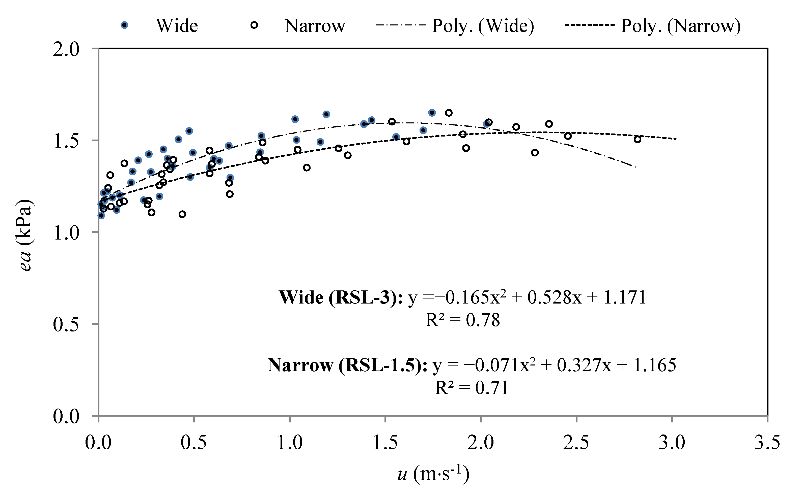
4.4. Relationships of Micrometeorological Variables

The magnitude of wind speed was different in wide and narrow RSL treatments. On a relatively windy day (DAP 47), the diurnal changes of u versus ea gave good agreement with a second degree polynomial fitting for both wide and narrow strips (Figure 7). The moving air flow that occurred deep in the lower part of the canopy can be explained the concentration of ea within the canopy. In other words, the lower layer of the plant canopy received a smaller supply of momentum, and removal of ea through transpiration was also lowered due to reduced penetration of radiation in the lower part of the canopy. Moreover, the sparse canopy structure of row planted maize under IRWH is poorly coupled to the atmosphere. This makes transpiration is likely to depend strongly on the interception of radiation by maize canopies with different tendencies of RSL. The effect of u on ea concentration was generally due to its influence on the resistance of boundary layer and the canopy, and soil surface resistance [29]. This implied that the loss of water vapor through Ev and Es by maize plants and from the soils surface of the basins and runoff strips depends on wind.
Figure 7. Daytime relationship between wind speed (u) and water vapor (ea) of all profile measurements (n = 40) on 6 February 2009 (47 DAP), on wide and narrow runoff strips.
Atmosphere 04 00428 g007
Figure 7 clearly illustrates that for both RSL treatments with increase in u, the concentration of ea within the canopy increased up to a certain level of ea (i.e., about 1.6 kPa). This peak was reached at a range of 1.4–1.8 ms−1 and 2.0–2.4 ms−1 for wide and narrow RSL treatments, respectively. This confirmed that the resulting variations in Ev and Es in the wide and narrow tillage of IRWH modified the airflow within the canopy, thus changing gradients in ea. In other words, indirectly Ev and Es rates were affected by the wind speed order of magnitude. The driving force for ET at any RSL is the gradient of ea and the resistance to ET processes is related to wind speed effect on ea concentration within the canopy. This can be explained in sparse planted maize under IRWH and is possibly referred to by the relationship of u and ea through the evaporative demand and on the drying power of the air within the canopy in both wide and narrow strips [7]. This meant that the wide RSL was faster to respond to evaporative demand of the atmosphere and supplied higher drying power of the air compared to narrow RSL treatments. In influencing Ev and/or Es within the plant canopy under the tillage system of IRWH, the key factor is the movement of air and turbulence, which is a function of wind speed, and that depends on the length of runoff strips. Increased movement of air within the plant canopy will result in higher ET rate [7]. Thus, a high wind speed has an implication in the control of ET, because wind operates the movement of saturated air in the plant canopy. On the contrary, under weak wind conditions, the air within the canopy may not move very much, raising the humidity of air around the canopy, such that the air tends to become saturated air unless it is replaced by drier air.

5. Conclusions

Knowledge of vertical profiles contributes to understanding variations in canopy structure of maize crop under IRWH and their roles in the energy fluxes to/from the canopy and soil surfaces. Results showed statistical differences of micrometeorological variables between the wide and narrow runoff strips. In wide runoff strips, lapse conditions extended from lowest measurement level (LP) to the upper middle section (MU) of the canopy, and inversion was apparent at the top of the canopy. The main difference observed on the wide runoff area was the temperature inversion at the top (UP) of the canopy during the midday hours and often close to isothermal conditions in the late morning. The higher air flow observed in the wide strips compared to narrow strips was the reason for the extension of temperature inversion into this part of the wide canopy. Thus, the Ev and Es within the canopy increased the ea concentration, but this was determined by the wind order of magnitude. The sparse maize canopy of the wide RSL had more drying power of the air in response to atmospheric evaporative demand compared to narrow RSL. Variation in air flow in wide and narrow runoff strips creates different gradients in ea for ET processes. Micrometeorological studies within canopy are encouraged to take advantage to understand that the equilibrium layer above the maize canopy under IRWH tillage system varies in response to wind caused more eddies and mixing in wide compared to the narrow strips. Results from this study verified the effect of wind on water vapor removal decreased downward as wind flow transfers within the canopy. This has an influence on the resistance of the boundary layer and canopy and soil surface resistance. Furthermore, vertical profile measurements will also assist to establish relationships between ET, soil water content, and soil surface resistance for dry and wet conditions. A comprehensive and good description of Ev and Es processes, therefore, necessitates a thorough study of the vertical profiles within sparse plant canopy.

Acknowledgments

This research was part of the project under “Radiation and Water Use Efficiency of Maize Production under in-field Rainwater harvesting (IRWH)” that was funded by University of the Free State under the Research Strategic Academic Cluster of Technology for Sustainable Crop Industries in Semi-Arid Regions, to whom the authors wish to express their gratitude.

Conflicts of Interest

The authors declare no conflict of interest.

References

  1. Hensley, M.; Bennie, A.T.P.; van Rensburg, L.D.; Botha, J.J. Review of “plant available water” aspects of water use efficiency under irrigated and dryland conditions. Water SA 2011, 37, 771–780. [Google Scholar]
  2. Botha, J.J.; Anderson, J.J.; Macheli, M.; van Rensburg, L.D.; van Staden, P.P. Water Conservation Techniques on Small Plots in Semi-Arid Areas to Increase Crop Yields. In Proceedings of Symposium/Workshop on Water Conservation Technologies for Sustainable Dryland Agriculture in Sub-Saharan Africa, Bloemfontein, South Africa, 8–11 April 2003; pp. 127–133.
  3. Joseph, L.F.; van Rensburg, L.D.; Botha, J.J. Technical Evaluation of Water Harvesting Techniques. In Review on Rainwater Harvesting and Soil Water Conservation Techniques for Crop Production in Semi-Arid Areas; Nova Science Publishers: New York, NY, USA, 2011; pp. 15–21. [Google Scholar]
  4. Stigter, C.J. Rural Response to Climate Change in Poor Countries. In Sustaining Soil Productivity in Response to Global Climate Change: Science, Policies, and Ethics; Sauer, T.J., Norman, J.M., Sivakumar, M.V.K., Eds.; Wiley-Blackwell: West Sussex, UK, 2010; pp. 35–38. [Google Scholar]
  5. Stigter, C.J.; Weiss, A. In quest of tropical micrometeorology for on-farm weather advisories. Agric. For. Meteorol. 1986, 36, 289–296. [Google Scholar] [CrossRef]
  6. Arya, S.P. Introduction to Micrometeorology, 2nd ed.; Academic Press: San Diego, CA, USA, 2001; p. 420. [Google Scholar]
  7. Tesfuhuney, W.A.; Walker, S.; van Rensburg, L.D. Comparison of energy available for evapotranspiration under in-field rainwater harvesting with wide and narrow runoff strips. Irrig. Drain. 2012, 61, 59–69. [Google Scholar] [CrossRef]
  8. Rosenberg, N.J.; Blad, B.L.; Verma, S.B. Air Temperature and Heat Transfer. In Microclimate: The Biological Environment; Wiley (Inter-Science): New York, NY, USA, 1983; pp. 124–133. [Google Scholar]
  9. Monteith, J.L; Unsworth, M.H. Principles of Environmental Physics, 2nd ed.; Edward Arnold: Sevenoaks, UK, 1990; p. 291. [Google Scholar]
  10. Ni, W. A coupled transilience model for turbulent air flow within plant canopies and the planetary boundary layer. Agric. For. Meteorol. 1997, 86, 77–105. [Google Scholar] [CrossRef]
  11. Meyers, T.; Paw U., K.T. Modelling the plant canopy micrometeorology with higher-order closure principles. Agric. For. Meteorol. 1987, 41, 143–163. [Google Scholar] [CrossRef]
  12. Savage, M.J.; Everson, C.S.; Metelerkamp, B.R. Evaporation Measurement above Vegetated Surfaces Using Micrometeorological Techniques; Report No. 349/1/97; Water Research Commission: Pretoria, South Africa, 1997. [Google Scholar]
  13. Stull, R.B. Mean Boundry Layer Characterstics. In An Introduction to Boundary Layer Meteorology; Kluwer Academic Publishers: Dordrecht, The Netherlands, 1988; pp. 7–21. [Google Scholar]
  14. Plate, E.J. Aerodynamic Characteristics of Atmospheric Boundary Layers; US Department of Energy: Springfield, CA, USA, 1971; p. 190.
  15. Busch, N.E. On the Mechanics of Atmospheric Turbulence. In Workshop on Micrometeorology; Haugen, D.A., Ed.; American Meteorological Society: Boston, MA, USA, 1973; pp. 1–65. [Google Scholar]
  16. Panofsky, H.A.; Dutton, J.A. Atmospheric Tturbulence: Models and Methods for Engineering Applications; John Wiley: New York, NY, USA, 1984; p. 397. [Google Scholar]
  17. Malek, E. Comparison of the Bowen ratio-energy balance and stability-corrected aerodynamic methods for measurement of evapotranspiration. Theor. Appl. Climatol. 1993, 48, 167–178. [Google Scholar] [CrossRef]
  18. Arya, S.P.S. Atmospheric Boundary Layer over Homogenous Terrain. In Engineering Meteorology; Plate, E.J., Ed.; Elsevier: New York, NY, USA, 1982; pp. 223–267. [Google Scholar]
  19. Campbell Scientific. CR10 Measurement and Control Mode, Instruction Manual; Campbell Scientific Ltd.: Leicestershire, UK, 1994; p. 187. [Google Scholar]
  20. SAS Institute Inc. SAS Enterprise Guide 4.1 (4.1.0.471), SAS Institute Inc.: Cary, NC, USA, 2006.
  21. Tesfuhuney, W.A. Optimizing Runoff to Basin Area Ratios for Maize Production with in-Field Rainwater Harvesting. Ph.D. Thesis, University of the Free State, Bloemfontein, South Africa, 2012. [Google Scholar]
  22. Shaw, R.H.; Schumann, U. Large-eddy simulation of turbulent flow above and within a forest. Bound.-Layer Meteorol. 1992, 61, 47–64. [Google Scholar] [CrossRef]
  23. Wilson, J.D.; Ward, D.P.; Thurtell, G.W.; Kidd, G.E. Statistics of atmospheric turbulence within and above a corn canopy. Bound.-Layer Meteorol. 1982, 24, 495–519. [Google Scholar] [CrossRef]
  24. Stigter, C.J.; Birnie, J; Jansen, P. Multi-point temperature measuring equipment for crop environment, with some results on horizontal homogeneity in a maize crop 1: Field results. Neth. J. Agric. Sci. 1976, 24, 223–237. [Google Scholar]
  25. Raupach, M.R. Anomalies in flux-gradient relationships over forest. Bound.-Layer Meteorol 1979, 16, 467–486. [Google Scholar]
  26. Denmead, O.T.; Bradley, E.F. On scalar transport in plant canopies. Irrig. Sci. 1987, 8, 131–149. [Google Scholar]
  27. Hernandez, G.; Trabue, S.; Sauer, T.; Pfeiffer, R.; Tyndall, J.C. Odor mitigation with tree buffers: Swine production case study. Agric. Ecosyst. Environ. 2012, 149, 154–163. [Google Scholar] [CrossRef]
  28. Jacobs, A.F.G.; Nieveen, J.P. Formation of dew and the drying process within crop canopies. Meteorol. Appl. 1995, 2, 249–256. [Google Scholar] [CrossRef]
  29. Ham, J.M.; Heilman, J.L. Aerodynamic and surface resistances affecting energy transport in a sparse crop. Agric. For. Meteorol. 1991, 53, 267–284. [Google Scholar] [CrossRef]

