Abstract
The air quality in Taiwan, at present, is determined by a pollution standard index (PSI) that is applied to areas of possible serious air pollution and Air Quality Total Quantity Control Districts (AQTQCD). Many studies, both in Taiwan and in other countries have examined the characteristics and levels of air pollution with PSI. This study uses air quality data collected from eight automatic air quality monitoring stations in an AQTQCD in central Taiwan and discusses the correlation between air quality variables with statistical analysis in an attempt to accurately reflect the difference of air quality observed by each monitoring station as well as to establish an air quality classification system suitable for the whole Taiwan. After using factor analysis (FA), seven air pollutants are grouped into three factors: organic, photochemical, and fuel. These three factors are the dominant ones in regards to the air quality of central Taiwan. Cluster analysis is used to classify air quality in central Taiwan into five clusters to present different characteristics and pollution degrees of air quality. This research results should serve as a reference for those involved in the review of air quality management effectiveness and/or the enactment of management control strategies.
1. Introduction
At present, the status of Taiwan’s air quality is communicated to the public with the Pollution Standards Index (PSI) which is based on a similar system created by the US Environmental Protection Agency (EPA). Taiwan first used the PSI in 1993 to measure air pollution levels by the ROC Environmental Protection Administration. PSI calculates the sub-index of pollutants based on the influence of five pollutants: particulate matter with a particle size below 10 microns (PM10), sulfur dioxide (SO2), nitrogen dioxide (NO2), carbon monoxide (CO), and ozone (O3), all of which are measured on a daily basis. The maximum values of the daily sub-index then are used as the PSI value measured by the monitoring station. The main purpose is to monitor the integral air quality of central Taiwan and suggest areas for improvement. Through the evaluation of PSI, local air quality statuses can be fully understood. The concentration levels of the five air pollutants are used to determine PSI which is then relayed as a number between 0 and 500 and classified into Good (0~50), Moderate (51~100), Unhealthy (101~199), Very Unhealthy (200~299), and Hazardous (≥300) levels. The ranges for PSI and pollutant concentration levels as well as PSI are shown in Table 1.

Table 1.
Comparison table of pollutant concentration and pollution sub-index.
| Pollutant | PM10 | SO2 | CO | O3 | NO2 |
|---|---|---|---|---|---|
| Statistics | 24-hour average | 24-hour average | Maximum 8-hour average within a 24-hour period | Maximum and minimum within a 24-hour period | Maximum and minimum within a 24-hour period |
| Unit | μg/m3 | ppb | ppm | ppb | ppb |
| PSI | |||||
| 50 | 50 | 30 | 4.5 | 60 | |
| 100 | 150 | 140 | 9 | 120 | |
| 200 | 350 | 300 | 15 | 200 | 600 |
| 300 | 420 | 600 | 30 | 400 | 1,200 |
| 400 | 500 | 800 | 40 | 500 | 1,600 |
| 500 | 600 | 1,000 | 50 | 600 | 2,000 |
Multivariate monitoring methods that consider all available data simultaneously can extract key information about the relationships and combined effects of air pollutants. When failures occur in air quality management systems, univariate monitoring methods are often inadequate in identifying causes because the signal-to-noise ratio is very low in each air pollutant measurement. However, multivariate monitoring can improve the signal-to-noise ratio through averaging, resulting in a more realistic evaluation of the environmental context [1,2,3,4]. In the field of chemometrics, multivariate statistical techniques have become one of the most active research tools in modeling and analysis over the last decade [5,6]. However, to the authors’ knowledge, only limited research on the effectiveness of multivariate models for the assessment and management of air pollution has been conducted thus far [7,8,9].
Air pollution is a well-known environmental problem associated with urban areas around the world. Various monitoring programs have been used to determine air quality by generating vast amounts of data on the concentration of each of the previously mentioned air pollutant in different parts of the world. The large data sets often do not convey air quality status to the scientific community, government officials, policy makers, and in particular to the general public in a simple and straightforward manner. This problem is addressed by determining the Air Quality Index (AQI) of a given area. AQI, which is also known as the Air Pollution Index (API) [10] or Pollutant Standards Index (PSI) [11], has been developed and disseminated by many agencies in the U.S. Canada, Europe, Australia, China, Indonesia, Taiwan, etc. [12,13].
Although more vigorous air pollution emission standards have been implemented in Taiwan to reduce emission of air pollutants, increasing numbers of manufacturing plants and various vehicles lead to no obvious improvement of the air quality in regions with concentrated sources of air pollution. As a result, it is necessary to promote air quality total quantity control strategies for further improvement in air quality. At present, the EPA in Taiwan has established 72 automatic air quality monitoring stations and divided Taiwan into seven Air Quality Total Quantity Control Districts. In the northern part, there is Hsinchu-Miaoli and the central part consists of Yunlin-Chiayi-Tainan, Kaohsiung-Pingtung, Yilan and Hualien-Taitung. It is expected that with the air quality total quantity control scheme of each district, seriously increasing air quality problems can be solved. Among these districts, the central part includes Taichung City, Changhua County and Nantou County.
This study explores eight existing air quality monitoring stations in central Taiwan. In accordance with the multivariate statistics method, this study selects seven important air pollutants to examine pollution levels, status, and air pollution characteristics and corresponding PSI as well as discusses the correlations between pollutants and distribution characteristics of air pollution at each monitoring station to accurately reflect the differences in air quality between monitoring stations. It is expected to serve as a reference to establish evaluations suitable to pollution characteristics and classification systems for air quality monitoring stations in Taiwan.
In accordance with the air population characteristics of the Air Quality Total Quantity Control District, as promulgated by the Environmental Protection Administration, Executive Yuan, Taiwan, seven air pollutants were selected in this study in order to comply with the Administration’s goal of formulating the emission standards policy. The research results also make it more legitimate and practicable for various air quality total quantity control districts in Taiwan to carry out air control in the future. Furthermore, the applied multivariate statistical analysis can determine the features of air pollution in each Air Quality Total Quantity Control District and the distribution characteristics among various clusters. Meanwhile, it can also prove the data collected from the original investigation. The statistical model, after investigation and verification, can be used to evaluate whether the effect of implementing air quality management achieving the target or not.
2. Methodology
2.1. Selection of the Air Quality Monitoring Stations
The EPA in Taiwan assigns Air Quality Total Quantity Control Districts according to geographic condition, industrial type, weather conditions and groups of municipalities or cities, as one district may be affected by the same air pollutants. This study selects eight automatic air quality monitoring stations in the part of the central district shown in Figure 1. Figure 2 is the geographic location of Taiwan in Asia.
Its administrative areas include Taichung City (Xitun station, Fengyuan station, Shalu station, Dali station), Changhua County (Changhua station, Erlin station) and Nantou County (Nantou station, Zhushan station). The air quality in this Air Quality Total Quantity Control District has long been ranked as a third air quality protection class while at present there is one major air pollution source, Taichung Thermal Power Plant, the world’s largest coal-fired power plant as well as one of the top two carbon emitters in the world. In addition, there are many factories located in Changhua Coastal Industrial Park, Changhua County; it brought impact on the air pollution quality in this area seriously.
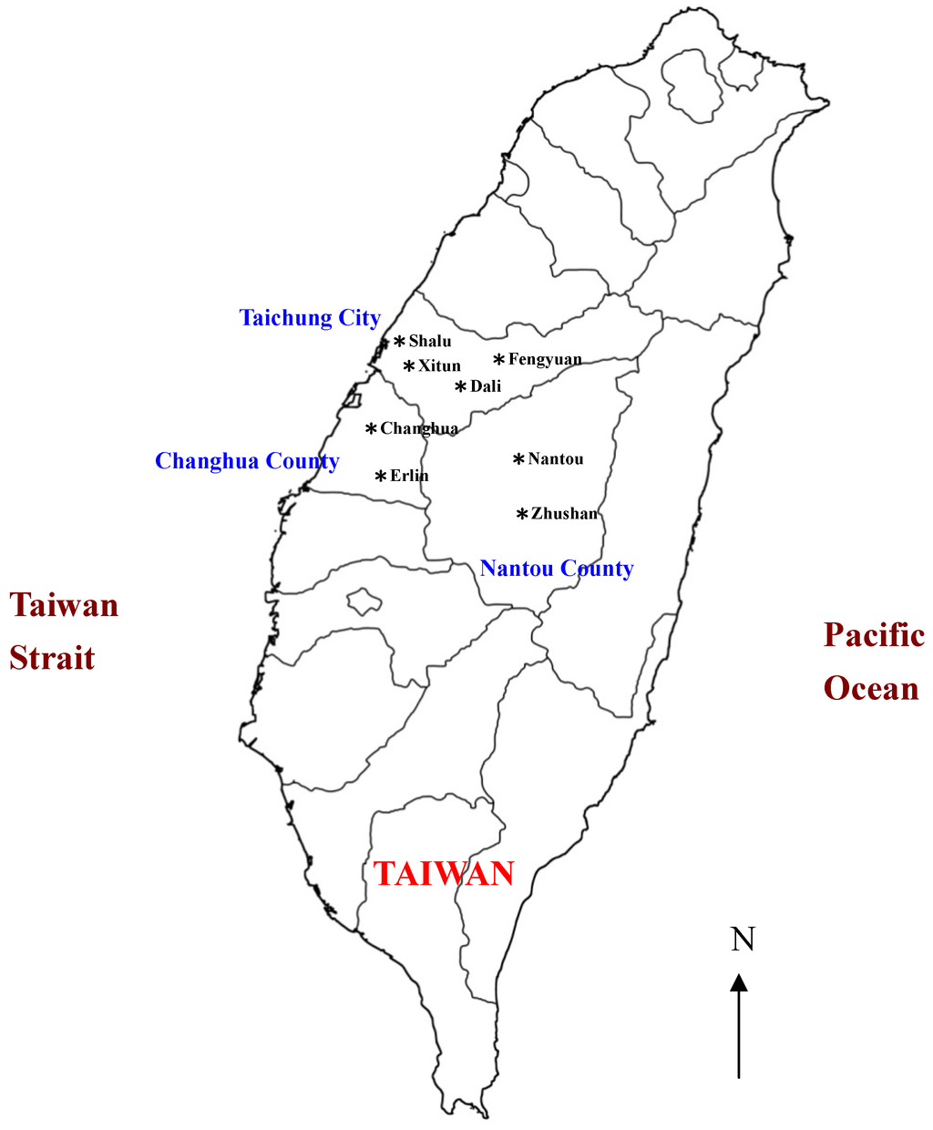
Figure 1.
Geographic locations of the eight Air Quality Monitoring Stations established by Environmental Protection Administration (Taiwan) in the study region.
2.2. Statistical Analyses—Factor Analysis
In order to select the elements to be included in the FA, a minimum of 70% of the samples need to have measurable levels of an element. In principle, FA actually groups the elements whose concentrations fluctuate together from one sample to another and separates these elements into factors [4,14,15,16]. Factor analysis is used for source apportionment in environmental data with the argument that elements that fluctuate together have some common characteristics. Ideally, each extracted factor represents a source affecting the samples. The factor analysis was conducted with the Statgraphics Plus program package (Statgraphics Manual 3.1, 1997). The initial components were rotated using the varimax method to obtain final eigenvectors with the most representatives of individual sources of variation. Although there are no well-defined rules on the number of factors to be retained, usually either factors that are meaningful or factors with eigenvalues greater than one are retained. In theory, irrelevant factors have zero eigenvalues and eigenvalues less than one indicate that a factor contributes less than a single variable. The physical meaning of the factors must be interpreted by observing which elements or variables display a high (≥0.25) loading within the factor. Loadings of less than 0.25 in absolute value may be dominated by random errors. There is not a set rule for the selection of the number of factors, but in application, the selected number of the factors must explain at least 70% of the total variance. Then the data are screened for outliers using their factor scores. The magnitude of a factor’s (i.e., source’s) influence on a specific sample is given by the factor score for that sample [17,18]. The factor score is the number of standard deviations from the mean of that factor as averaged over all the samples; in other words, it is the value of the factor. An average contribution from the factor results in a score of zero, a larger than average contribution results in a positive score and a lower than average contribution results in a negative score. Factor scores greater than one indicate a strong influence of that source or factor on that individual sample.
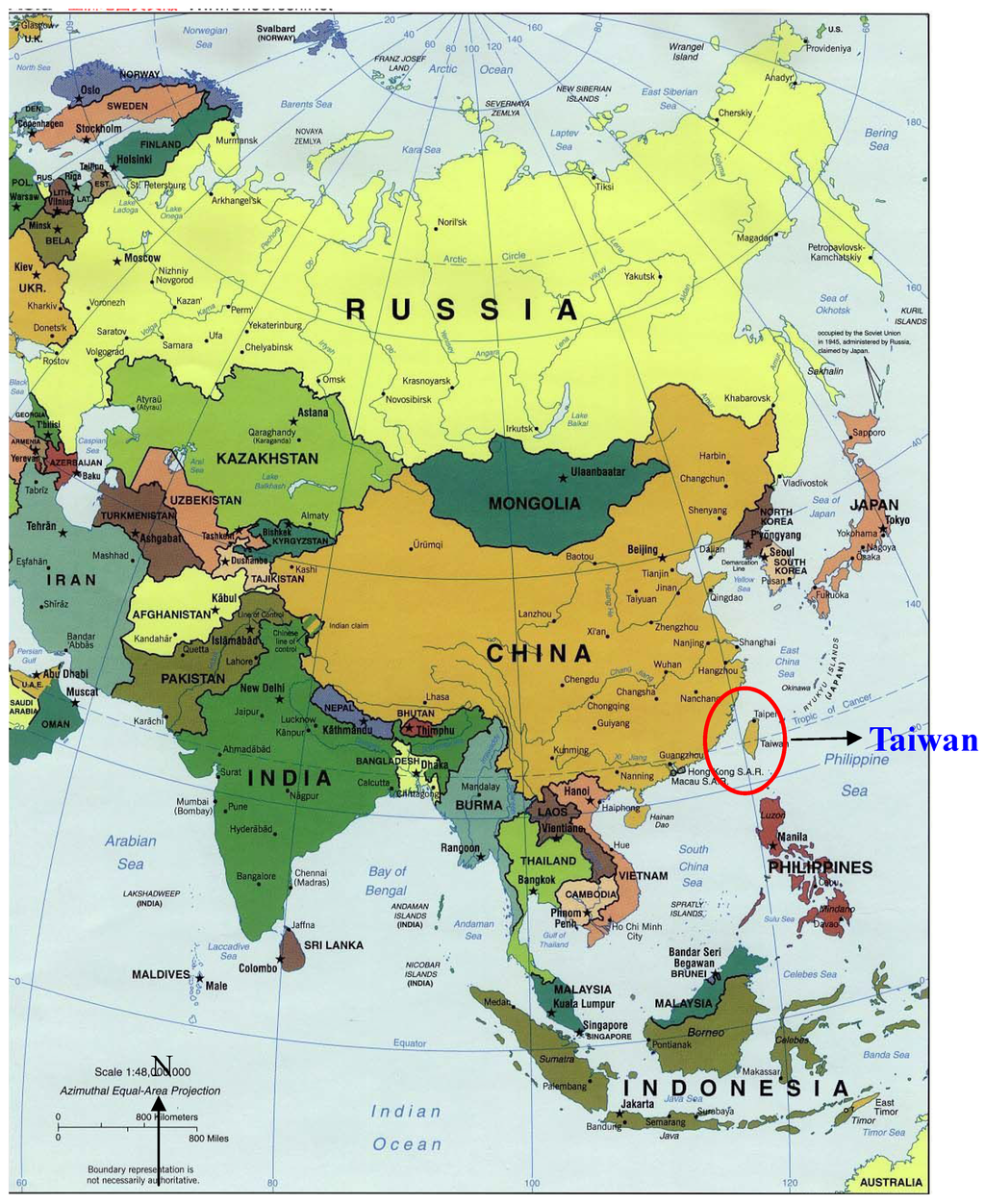
Figure 2.
The geographic location of Taiwan in Asia.
2.3. Cluster Analysis
Cluster analysis is an exploratory data analysis tool for solving classification problems. Its objective is to sort cases into groups, or clusters, so that the degree of association is strong between members of the same cluster and weak between members of different clusters. Each cluster thus describes, in terms of the data collected, the class to which its members belong; and this description may be abstracted through use from the particular to the general class or type. Hierarchical agglomerative clustering is the most common approach as it provides intuitive similarity relationships between any one sample and the entire dataset. It is typically illustrated by a dendrogram (tree diagram) [19,20]. The dendrogram provides a visual summary of the clustering processes, presenting a picture of the groups and their proximity, with a dramatic reduction in dimensionality of the original data. Additionally, cluster analysis helps in grouping objects (cases) into classes (clusters) on the basis of similarities within a class and dissimilarities between different classes. The class characteristics are not known in advance but maybe determined from the analysis. The results of CA help in interpreting the data and indicate patterns [6,21].
2.4. Discriminant Analysis
Discriminant analysis is used to determine the variables that discriminate between two or more naturally occurring groups. It uses raw data to construct a discriminant function for each group [22] as in Equation (1):
 where i is the number of groups (G), ki is the constant inherent to each group, n is the number of parameters used to classify a set of data into a given group, wj is the weight coefficient assigned by DA to a given selected parameter (pj). In this case study, three groups of temporal (three seasons) and spatial (three sampling regions) evaluations have been selected and the number of analytical parameters used to assign a measure from a monitoring site into a group (season or spatial) has been taken as n. Discriminant analysis is applied to the raw data by using the standard, forward stepwise and backward stepwise modes to construct discriminant functions to evaluate both the spatial and temporal variations in air quality. The temporal (season) and the spatial (site) were the grouping (dependent) variables, while all the measured parameters constituted the independent variables.
3. Results and Discussion
3.1. Selection Time and Range of Monitoring Data
In order to obtain complete and diversified pollutant data, this study considers seven pollutants including SO2, NO2, CO, PM10, O3, total hydrocarbon compounds (THC) and non-methane hydrocarbon compounds (NMHC) for factor analyses to identify the major factors of air quality statuses in the Air Quality Total Quantity Control District. The selected series data mainly come from the website of Taiwan’s EPA (http://www.epa.gov.tw) for the period between 1 January 2010 and 30 September 2011. During this period, some data are incompletely collected because of un-expected instrument down time for repair and maintenance; all of the incomplete data sets are deleted so that there are 610 sets of daily air pollution samples. All statistical analyses were carried out with SPSS for Windows, version 17.0.
3.2. Results of the Factor Analysis
3.2.1. Selecting the Factor Analysis Results
In the factor analysis implemented in this study, the maximum varimax rotation is used to carry out orthogonal rotation to explain the number characteristics of factors. As shown in the analysis results, there are three factors with the eigenvalues greater than one in Table 2. Their accumulated total variance explained is 66.212%. The eigenvalues of the three factors are 1.837, 1.522 and 1.013, respectively. These three factors are selected to illustrate the major factors that affect the air quality for the Air Quality Total Quantity Control District.
Table 2.
Results factor analyses and the variances.
| Components | Initial Eigenvalues | % of Total Variance | Cumulative Variance % |
|---|---|---|---|
| 1 | 1.837 | 27.931 | 27.931 |
| 2 | 1.522 | 22.563 | 50.494 |
| 3 | 1.013 | 15.718 | 66.212 |
| 4 | 0.945 | 10.750 | 76.962 |
| 5 | 0.750 | 9.807 | 86.769 |
| 6 | 0.578 | 7.114 | 93.883 |
| 7 | 0.287 | 6.117 | 100.000 |
3.2.2. Determination of Factors
The number of major factors can be decided from the number of eigenvalues greater than one. Table 3 shows the component matrix table after orthogonal rotation in order to describe the characteristics of each factor. It can be used to describe differences between the concentration levels of each air pollutant in the Air Quality Total Quantity Control District.
Table 3.
Matrix of air quality factor loadings for the Air Quality Total Quantity Control District.
| Pollutants | Factors | ||
|---|---|---|---|
| 1 | 2 | 3 | |
| NMHC | 0.876 | −8.159E-02 | −7.255E-02 |
| THC | 0.807 | 0.146 | 0.466 |
| NO2 | 7.034E-02 | 0.866 | 4.625E-02 |
| PM10 | 9.265E-02 | 0.751 | −5.322E-03 |
| O3 | −4.046E-02 | 0.691 | 7.378E-02 |
| SO2 | 5.873E-02 | −0.139 | 0.872 |
| CO | −1.309E-02 | 0.232 | 0.754 |
Factor 1
Factor 1 is composed of NMHC and THC. Their total variance as shown in Table 2 reaches 27.931%.
Factor loadings of NMHC in Factor 1 in Table 3 reach 0.876 while those of THC are 0.807. These two have very similar and approximate loading factors that show a relatively high correlation between these two pollutants. These volatile organic compounds mainly come from industrial activities and vehicle fuel in the Air Quality Total Quantity Control District. Among them, non-NMHC generates photochemical reaction. They further form important air pollutant such as ozone and it is likely that they further react and form secondary PM10 and pose a serious threat to the respiratory systems of humans [23]. Under the reactions of active oxygen containing free radicals such as atomic oxygen, ozone, and hydrogen atoms, organic compounds including NMHC and THC generate a series of chemical compounds including aldehyde, ketone, alkane, alkene and the important intermediate free radicals that facilitate the production of NO2 via the oxidization of NO. This results in the production of the secondary pollutants of smog such as O3, aldehyde, and peroxyacyl nitrates (PAN). Additionally, NMHC produced from volatile or burning fuels will react with O3 or oxygen in atomic states to further produce aldehyde compounds [24]. In short, NMHC and THC are both volatile organic compounds and although they have low toxicity to humans, they do contribute to air pollution in the district. Therefore, Factor 1 has been called “Organic Pollution Factor.”
Factor 2
Factor 2 consists of NO2, PM10 and O3 with total variance in Table 2 reaching 22.563%.
Among the factor loadings shown in Table 3, NO2 has the highest loading with 0866. The main source of NO2 comes from vehicle emissions, fossil fuel power plants and other industrial producers. During combustion, NO is generated and oxygen in the air immediately oxidizes NO to form NO2. NO2 is also an important indicator of the source of air pollution. But when there is no wind, NO emitted by vehicles accumulates in the air to trigger a photochemical reaction resulting in the composition of smog pollutants.
Among the loadings of Factor 2 in Table 3, PM10 is also found with a high level of 0.751 and is therefore an important indicator of air pollution. PM10 in the atmosphere comes mainly from two types: primary aerosols and secondary aerosols. Primary aerosols are emitted directly by human emission sources (factories and vehicle emissions) as well as from non-human emission sources (street and soil dust and salt from the nearby sea). These particles, due to the scattered sunlight, influence visibility [25]. This is especially clearly observed when relative humidity is high. If NO2 and other irritant gases have high concentration levels, they combine with PM10 to jointly form brown smog, a serious indicator of air pollution. Among air pollutants, PM10 is considered a major indicator pollutant. In the Air Quality Total Quantity Control District that is the subject of this study, Taichung Thermal Power Plant is the greatest source of PM10 in the atmosphere.
The O3 loading of Factor 2 in Table 3 is 0.691. In Taiwan, besides the contributing pollutant, PM10, to air pollution, O3 is also another leading pollutant. In busy cities, heavy traffic produces high concentration levels of ozone and sometimes, yellow-brownish “smog” can be observed due to the generation of nitrides caused by the fuel combustion of vehicles resulting in NO and NO2. O3, at the same time, reacts with NMHC and produces smog through a photochemical reaction. O3 is an important indicator of air pollution and greatly contributes to air pollution.
To sum up, NO2, PM10 and O3 are major pollutants that tie closely with photochemical oxidization. Although some environmental engineering textbooks indicate that the production of PM10 is not directly related to the production of O3, Chou [25] has pointed out that the secondary aerosols of photochemical reactions cause high levels of atmospheric PM2.5 and PM10 in Taiwan. Chen and Lee [26] have observed that secondary organic aerosols and photochemical reactions of VOCs are closed related to the formation of atmospheric O3. Based on these observations, the production of PM10 should be considered to be closely related to the photochemical reactions of atmospheric pollutants. The Factor 2 is called “Photochemical Pollution Factor.”
Factor 3
Factor 3 consists of SO2 and CO with a total variance reaching 15.718% as shown in Table 2.
In Factor 3, SO2 has a relatively high loading of 0.872. SO2 is mainly produced from the combustion of fuel containing sulfur. In this study district, due to the popularity of diesel fuel vehicles as well as the influence of industrial discharged pollutants, SO2 has become a major contributor to air pollution. Additionally, SO2 is generated by Taichung Thermal Power Plant as it burns coal, thereby making it an important source of this type of air pollution.
The CO loading of Factor 3 in Table 3 is 0.754. Statistical analysis shows that 86% of CO in the atmosphere is emitted from vehicles and only a small portion comes from the incompletely burned fuel of factories and the power plant due to gases generated from the incomplete combustion of carbon containing fuel. CO is also an important air pollution source indicator and the pollutant with the highest concentration level in the air. In the study district, air pollution sources are influenced by vehicles and point pollution and that leads to high CO levels in the atmosphere.
In summary, SO2 and CO are the main results of fuel combustion. The fuel required during combustion is, in particular, a fixed pollution source such as creosote, coal, coking coal used for fuel in factories and the diesel engines of vehicles that generate the major pollutant, SO2. Due to a lack of oxygen, incomplete combustion leads to the production of CO. As a result, Factor 3 is called “Fuel Factor.”
3.3. Analysis of Air Pollution Characteristics—Cluster and Discriminant Analysis
For the cluster analysis, this study adopts a two-staged clustering algorithm to acquire approximate cluster results via hierarchical methods and then different cluster numbers are tested with the K-mean method. As a result, five clusters are selected to classify the differences in air quality. The relationship between clusters and factors are indicated in Figure 3. Among various air pollutants, there are some common characteristics. If these can be understood, it would benefit the analyses of the changes of characteristics of air quality pollution. Table 4 shows the characteristics listed below.
3.3.1. Cluster 1
This cluster is shown in Table 4 as having the highest concentration level of NO2 among all of the five clusters. However, the score in the photochemical pollution factor (Figure 3) ranks it third because the PSI range is between 0 and 100. According to Table 1, NO2, at present, has no corresponding environmental air quality standards. When NO2 concentration reaches 600 ppb, its corresponding PSI is 200. The study district has a high concentration level of NO2 at 497.9 ppb, yet there is no corresponding change to PSI. Therefore, it influences the level of photochemical pollution factor in this cluster less significantly than that in Clusters 4 and 5. However, if the concentration of NO2 is high, the concentration of NO is also high. For example, the emission of NO from vehicles accumulated in the atmosphere occur oxidation reaction in photochemistry and it has become one of the pollutants of photochemical smog. The resulting pollution level is significant. In addition, this cluster has the third highest organic pollution factor and fuel factor with an average THC concentration level of 2.18 ppb and NMHC of 0.49 ppb while the average SO2 concentration level in the fuel factor is 20.74 ppb and CO is 1.13 ppm. Scores of factors in this cluster are ranked third and lies in the air quality standard between good to unhealthy. Based on this cause, this cluster can be determined to experience “serious air pollution.”
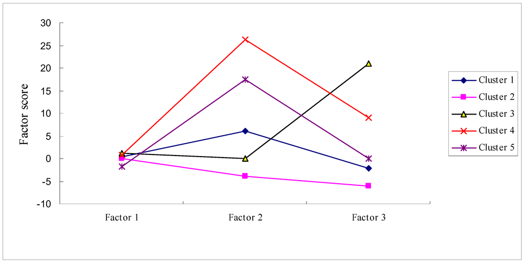
Figure 3.
Factor scores of the five clusters.
Table 4.
The average and the extreme value of each pollutant among the clusters.
| Cluster | Cluster 1 | Cluster 2 | Cluster 3 | Cluster 4 | Cluster 5 |
|---|---|---|---|---|---|
| Number | |||||
| Item | |||||
| O3(ppb) | 34.87 | 23.89 | 42.34 | 37.16 | 165.91 |
| 5~74.9 | 0.15~92.45 | 7.07~89.71 | 1.46~98.64 | 93.50~398.35 | |
| NO2(ppb) | 422.14 | 38.28 | 48.40 | 74.69 | 56.81 |
| 264.5~497.9 | 0.15~212.05 | 0.65~97.92 | 0.81~236.90 | 15.16~117.23 | |
| PM10(μg/m3) | 98.97 | 78.36 | 107.99 | 167.03 | 125.91 |
| 48~157.3 | 1.02~136.12 | 45.36~217.05 | 99.54~458.18 | 59.46~230.51 | |
| SO2(ppb) | 20.74 | 19.32 | 102.27 | 27.88 | 19.79 |
| 7.59~35.38 | 0.2~88.55 | 48.62~324.90 | 2.69~100.39 | 6.04~38.82 | |
| CO(ppm) | 1.13 | 1.17 | 1.42 | 1.62 | 1.39 |
| 0.6~1.74 | 0.01~8.60 | 0.75~4.07 | 0.45~25.86 | 0.72~6.10 | |
| THC(ppb) | 2.18 | 2.02 | 2.09 | 2.22 | 2.06 |
| 1.32~2.94 | 0.6~6.64 | 1.23~3.35 | 0.68~3.86 | 1.06~3.03 | |
| NMHC(ppb) | 0.49 | 0.60 | 0.75 | 0.64 | 0.51 |
| 0.17~0.94 | 0.008~5.44 | 0.24~1.78 | 0.006~2.15 | 0.11~1.52 | |
| Air Quality Standards | Good ~ Unhealthful | Good ~ Meoderate | Moderate ~ Very Unhealthful | Moderate~ Hazardous | Moderate ~ Very Unhealthful |
| Daily Statistics | 12 | 305 | 37 | 236 | 20 |
3.3.2. Cluster 2
Figure 3 shows that the factor scores of this cluster have the lowest rankings for photochemical pollution factor and fuel factor as well as the second lowest ranking of organic pollution factor. This indicates good air quality within this cluster. As shown in Table 4, this cluster has lower concentration levels of air pollutants than other clusters and there have been no sudden increases. As a result, the air quality standards mostly fall between good and moderate, most of time it is the latter. If PM10 is between 50 and 150 μm/m3, air quality standards are determined to be moderate. PM10 in this cluster is usually higher than 50 μm/m3 while concentration levels of other air pollutants remain low. The above analysis results categorize this cluster as “light air pollution.”
3.3.3. Cluster 3
As indicated by Figure 3, this cluster has the highest fuel factor score but the fourth highest photochemical pollution factor score. Table 4 shows that the average SO2 concentration level in the fuel factor in Cluster 3 is 102.27 ppb, the highest among all clusters and CO at 1.42 ppm, the second highest among all clusters. The concentration level of SO2 is between 48.62 and 324.90 ppb, indicating that it is significantly influenced by fuel factor to some degree. This cluster merely has the fourth highest photochemical pollution factor score with an average NO2 concentration level at 48.4 ppb, PM10 at 107.99 μm/m3, and O3 at 42.34 ppb. This shows an insignificant increase in the concentration level of photochemical pollution factor in areas with high fuel factor loadings. The air quality standards of the cluster are between moderate and very unhealthy and are considered moderate most of the time. Winter is when the air quality standards are very unhealthy with an average concentration level of SO2 over 24 h reaching 324.9 ppb. In addition, this cluster also has some days when PM10 concentration is higher than 150 μm/m3 resulting in unhealthful air quality standards. The above analysis allows to conclude that this cluster experiences “serious fuel factor air pollution.”
3.3.4. Cluster 4
This cluster in Figure 3 has a photochemical pollution factor score that is, abnormally high as well as the second highest organic pollution factor and fuel factor scores. This indicates seriously air pollution. Table 4 shows that the average concentration level of PM10 at 167.03 μm/m3 is the highest among all clusters, NO2 at 74.69 ppb is the second highest among all clusters, and O3 at 37.16 ppb is the third highest among all clusters. This study district is near the Taichung Thermal Power Plant, an area vulnerable to air pollution, especially PM10. Thus, PSIs are often at the high levels. In this cluster, on most days, the average 24-hour PM10 exceeds 150 μm/m3. Moreover, even higher PM10 concentration levels are identified between late autumn and early spring. The highest concentration level on these days reached 458.18 μm/m3 and the air quality standards are at a hazardous level. In this cluster, fuel factor also has high scores with an average SO2 concentration level at 27.88 ppb, the highest among all clusters as well as CO at 1.62 ppm, the highest among all clusters. Among them, the maximum average 8-hour CO once reached 25.86 ppm resulting in hazardous levels of air quality. In addition, this cluster has the second highest organic pollution factor score with an average THC concentration level at 2.22 ppb, the highest among all clusters as well as NMHC at 0.49 ppb, the second highest among all clusters. But because organic pollution factor is not clearly defined in PSI, it only has a minor influence in air pollution. The air quality standards of this cluster are between moderate to hazardous, and on most days, they are considered hazardous. The above analysis allows us to conclude that this cluster has “very serious photochemical pollution.”
3.3.5. Cluster 5
Figure 3 shows that this cluster has the second highest photochemical pollution factor score, the third highest fuel factor score, and the lowest organic pollution factor score. In Table 4, this cluster has an average O3 concentration level in the photochemical pollution factor at 165.91 ppb, the highest score among all clusters. NO2, at 56.81 ppb, has the third highest score among all clusters and PM10, at 125.91 μm/m3, has the second highest score among all clusters. In this cluster, O3 is a major air pollutant with a maximum hourly concentration level higher than 120 ppb resulting in air quality standards considered as unhealthy. The average concentration of NO2 in this cluster is not high and there are not many days in which the level of PM10 exceeds 150 μm/m3. In terms of fuel factor, the average NO2 concentration is 19.79 ppb, the fourth highest score among all clusters. CO, at 1.39 ppm, has the second highest score among all clusters but it has less influence on air pollution than the photochemical pollution factor. It is worth noting that for photochemical pollution factors, Cluster 4 scored about 26.3 and Cluster 5 scored 17.5; Cluster 4 has more influence on air pollution than Cluster 5 because in Cluster 4, PM10 is the major pollutant with more days at higher concentration levels (236 days) than those in Cluster 5 (20 days) with O3 as its primary pollutant. These two pollutants are major factors that contribute to serious air pollution and in Cluster 1 there were only 12 days that had higher concentration levels of NO2 than these two clusters. As mentioned above, the NO2 concentration range is between PSI 0 and 100 and at present, there are no corresponding environmental air standards. Therefore, it does not significantly influence the level of air pollution in Clusters 4 and 5 so the air quality standards are considered to be between moderate and very unhealthy for a total of 20 days. Among these days, 6 days were very unhealthy due to high O3 concentration levels. In short, this cluster is regarded as having “serious photochemical pollution” issues.
3.3.6. Discriminant Analysis
Discriminant analysis is a method used to determine objectively the category of a new sample based on a known classification and the collected characteristics of a certain quantity. It is carried out to calculate the centroid of each cluster, or the intersection of individual discriminant parameters, using the discriminant quantity obtained in a study. The value of this calculated centroid represents the unique characteristics of each cluster; the discriminant parameters in the cluster are then combined linearly to calculate the discriminant function.
This study uses various discriminant parameters combination tests as well as discriminant analyses. First, seven air pollutants are selected as discriminant parameters. The actual cluster levels are then decided according to the results of previous cluster analysis; the coefficient of the discriminant function is introduced to acquire the ratio of each monitoring station and the discriminant clusters. Cross comparisons of the discriminant clusters and actual clusters are conducted to determine how they are different.
Table 5 shows the test results for each cluster after discriminant analysis with a high fitness of discriminant clusters acquired with a discriminant function and actual clusters acquired with cluster analysis (the percentage of discriminant accuracy). Among them, Clusters 1, 2, 3, 4, 5, respectively reaches 100%, 93.44%, 86.48%, 97.45%, and 95.00%, with a total fitness of 94.75%, very accurate results. In particular, Clusters 1, 4, and 5 feature serious photochemical pollution with an accuracy percentage higher than 95.00%, indicating that the error percentage for the determination of serious photochemical pollution and very serious photochemical pollution is low. Hence, the cluster analyses are acceptable.
Table 5.
Results of discriminant analysis for each cluster.
| Discriminant Analyses | Cluster 1 | Cluster 2 | Cluster 3 | Cluster 4 | Cluster 5 | Discriminant Accuracy% | |
|---|---|---|---|---|---|---|---|
| Actual Cluster | |||||||
| Cluster 1 | 12 | 0 | 0 | 0 | 0 | 12/12*100 = 100 | |
| Cluster 2 | 0 | 285 | 7 | 13 | 0 | 285/305*100 = 93.44 | |
| Cluster 3 | 0 | 2 | 32 | 3 | 0 | 32/37*100 = 86.48 | |
| Cluster 4 | 1 | 2 | 3 | 230 | 0 | 230/236*100 = 97.45 | |
| Cluster 5 | 0 | 0 | 0 | 1 | 19 | 19/20*100 = 95.00 | |
| Total | 13 | 289 | 42 | 247 | 19 | 578/610*100 = 94.75 | |
4. Conclusion
This study uses air quality data from eight automatic air pollution monitoring stations in central Taiwan as well as multivariate statistical methods to examine the correlation among air quality variables with the expectation of truly reflecting the difference of air quality surrounding each monitoring station. First, factor analysis shows that there are organic pollution, photochemical pollution and fuel factors that dominate air quality. In terms of cluster analysis, this study categorizes the air quality of the Air Quality Total Quantity Control District in central Taiwan into 5 clusters. All 5 clusters have an average discriminant accuracy of 94.75% after discriminant analysis. This study incorporates relevant PSI information released by the EPA of Taiwan in order to effectively assess the air quality of the Air Quality Total Quantity Control District in central Taiwan as well as serve as a reference for governmental authorities to manage applications and approvals regarding air quality models, make efforts to improve air quality, and enact other relevant strategies.
When carrying out the factor analysis, the features and levels of air pollution in Air Quality Total Quantity Control District cannot be recognized. After applying the cluster analysis, the features and levels of air pollution in Air Quality Total Quantity Control District can then be known. PSI information can also determine the level of air pollution from each cluster. Finally, by using SPSS and cluster analysis, high recognition rate can be acquired and it verified the accuracy resulted in cluster analysis.
The authors trust that applying the multivariate statistical analysis as well as the application of PSI in each cluster which explored the level of air pollution has to achieve the policy target of management system in Air Quality Total Quantity Control District. It also has to satisfy the indicator system purpose and management target of the accurate implementation so that required various management information can be exactly reflected in order to conform to the Air Quality Total Quantity Control District. However, the results are also a practical methodology for readers who possess basic concept of statistics and multivariate statistical analysis. In this study, the ultimate objective is to establish the air pollution characteristics for each monitoring station and a system suitable for classifying the air quality in Taiwan. The results will be valuable references to be used by air quality monitoring stations for improving the monitoring of air quality in Taiwan. Besides, the results obtained in this study by coping with the PSI data published by Taiwan Environmental Protection Administration are effective in judging the air quality of the Central Taiwan Total Quantity Control District; they are also valuable references to assist in future management.
Acknowledgments
The authors gratefully acknowledge the support of the National Science Council of Taiwan under Grant NSC-2011-2221-E-214-011 and I-Shou University under ISU-102-02-01. The authors also deeply appreciate the editor and the anonymous reviewers for their insightful comments and suggestions.
Conflicts of Interest
The authors declare no conflict of interest.
References
- Shirodkar, P.V.; Mesquita, A.; Pradhan, U.K.; Verlekar, X.M.; Babu, M.T.; Vethamony, P. Factors controlling physico-chemical characteristics in the coastal waters off Mangalore—A multivariate approach. J. Environ. Res. 2009, 109, 245–257. [Google Scholar] [CrossRef]
- Stenberg, M.; Linusson, A.; Tysklind, M.; Andersson, P.L. A multivariate chemical map of industrial chemicals: Assessment of various protocols for identification of chemicals of potential concern. Chemosphere 2009, 76, 878–884. [Google Scholar] [CrossRef]
- Zhang, X.; Wang, Q.; Liu, Y.; Wu, J. Application of multivariate statistical techniques in the assessment of water quality in the Southwest New Territories and Kowloon, Hong Kong. Environ. Monit. Assess. 2011, 173, 17–27. [Google Scholar] [CrossRef]
- Martinez, M.A.; Caballero, P.; Carrillo, O.; Mendoza, A.; Mejia, G.M. Chemical characterization and factor analysis of PM2.5 in two sites of monterrey, Mexico. J. Air Waste Manag. Assoc. 2012, 62, 817–827. [Google Scholar] [CrossRef]
- Charlton, A.J.; Robb, P.; Donarski, A.J.; Godward, J. Non-targeted detection of chemical contamination in carbonated soft drinks using NMR spectroscopy, variable selection and chemometrics. Anal. Chim. Acta. 2008, 618, 196–203. [Google Scholar] [CrossRef]
- Tobiszewski, M.; Tsakovski, S.; Simeonov, V.; Namieśnik, J. Surface water quality assessment by the use of combination of multivariate statistical classification and expert information. Chemosphere 2010, 80, 740–746. [Google Scholar] [CrossRef]
- Liu, P.W.G. Establishment of a Box-Jenkins multivariate time-series model to simulate ground-level peak daily one-hour ozone concentrations at Ta-Liao in Taiwan. J. Air Waste Manag. Assoc. 2007, 57, 1064–1074. [Google Scholar]
- Pires, J.C.M.; Sousa, S.I.V.; Pereira, M.C.; Alvim-Ferraz, M.C.M.; Martins, F.G. Management of air quality monitoring using principal component and cluster analysis-part II: CO, NO2 and O3. Atmos. Environ. 2008, 42, 1261–1274. [Google Scholar]
- Yalcin, M.G.; Tumuklu, A.; Sonmez, M.; Erdag, D.S. Application of multivariate statistical approach to identify heavy metal sources in bottom soil of the Seyhan River (Adana), Turkey. Environ. Monit. Assess. 2010, 164, 311–322. [Google Scholar] [CrossRef]
- Murena, F. Measuring air quality over large urban areas: Development and application of an air pollution index at the urban area of Naples. Atmos. Environ. 2004, 38, 6195–6202. [Google Scholar] [CrossRef]
- EPA (Environmental Protection Agency). Measuring Air Quality. The Pollutant Standards Index; EPA 451/K-94–001; EPA: Research Triangle Park, NC, USA, 1994; p. 73. [Google Scholar]
- Cairncross, E.K.; John, J.; Zunckel, M. A Novel Air pollution index based on the relative risk of daily mortality Associated with Short-term Exposure to Common Air Pollutants. Atmos. Environ. 2007, 41, 8442–8454. [Google Scholar] [CrossRef]
- Cheng, W.; Chen, Y.; Zhang, J.; Lyons, T.J.; Pai, J.; Chang, S. Comparison of revised air quality index with the PSI and AQI indices. Sci. Total Environ. 1999, 382, 191–198. [Google Scholar]
- Collier, K.J. Linking multimetric and multivariate approaches to assess the ecological condition of streams. Environ. Monit. Assess. 2009, 157, 113–124. [Google Scholar] [CrossRef]
- Yang, Y.H.; Zhou, F.; Guo, H.C.; Sheng, H.; Liu, H.; Dao, X.; He, C.J. Analysis of spatial and temporal water pollution patterns in Lake Dianchi using multivariate statistical methods. Environ. Monit. Assess. 2010, 170, 407–416. [Google Scholar] [CrossRef]
- Arrebola, J.P.; Mutch, E.; Cuellar, M.; Quevedo, M.; Claure, E.; Mejía, L.M.; Fernández-Rodríguez, M.; Freire, C.; Olea, N.; Mercado, L.A. Factors influencing combined exposure to three indicator polychlorinated biphenyls in an adult cohort from Bolivia. J. Environ. Res. 2012, 116, 17–25. [Google Scholar] [CrossRef]
- Serpil, Y.K.; Semra, G.T. Source apportionment of atmospheric trace element deposition. Environ. Eng. Sci. 2008, 25, 1263–1271. [Google Scholar] [CrossRef]
- Ratola, N.; Amigo, J.M.; Alves, A. Comprehensive assessment of pine needles as bioindicators of PAHs using multivariate analysis. The importance of temporal trends. Chemosphere 2010, 81, 1517–1525. [Google Scholar] [CrossRef]
- Einax, J.W.; Truckenbrodt, D.; Kampe, O. River pollution data interpreted by means of chemometric methods. Microchem. J. 1998, 58, 315–324. [Google Scholar] [CrossRef]
- McKenna, J.E., Jr. An enhanced cluster analysis program with bootstrap significance testing for ecological community analysis. Environ. Model. Softw. 2003, 18, 205–220. [Google Scholar] [CrossRef]
- Vega, M.; Pardo, R.; Barrado, E.; Deban, L. Assessment of seasonal and polluting effects on the qualityof river water byex ploratory data analysis. Water Res. 1998, 32, 3581–3592. [Google Scholar] [CrossRef]
- Wunderlin, D.A.; Diaz, M.P.; Arne, M.V.; Pesce, S.F.; Hued, A.C.; Bistoni, M.A. Pattern recognition techniques for the evaluation of spatial and temporal variations in water quality: A case study: Suquia river basin (Cordoba-Argentina). Water Res. 2001, 35, 2881–2894. [Google Scholar] [CrossRef]
- Chang, S.C.; Lee, C.T. Secondary aerosol formation through photochemical reactions rstimated by using air quality monitoring data in Taipei city from 1994 to 2003. Atmos. Environ. 2007, 41, 4002–4017. [Google Scholar] [CrossRef]
- McElory, W.J.; Waygood, W.J. Oxidation of formaldehyde by the hydroxyl radical in aqueous solution. J. Chem. Soc. 1991, 87, 1513–1521. [Google Scholar]
- Chou, T.G. The Research of Air Quality Management in Fine Particulate Matters; (in Chinese). Academia Sinica Research Weekly 1276; Central Office of Administration: Taiwan, 2010. [Google Scholar]
- Chen, W.K.; Lee, C.T. The Establishment of Aerosol Control Mode Based on the Photochemical Reaction Mechanism; (in Chinese). NSC-1999-EPA-Z-231–001; National Science Council: Taiwan, 1999. [Google Scholar]
© 2013 by the authors; licensee MDPI, Basel, Switzerland. This article is an open access article distributed under the terms and conditions of the Creative Commons Attribution license (http://creativecommons.org/licenses/by/3.0/).