Case Study of Pollutants Concentration Sensitivity to Meteorological Fields and Land Use Parameters over Douala (Cameroon) Using AERMOD Dispersion Model


Abstract
: This paper deals with the simulation of the NOx concentration over Douala for the period 2002–2006 by means of the American Meteorological Society (AMS)/Environmental Protection Agency (EPA) Regulatory Model (AERMOD) model, version 07026. Its sensitivity to local meteorological fields and land use parameters are investigated by selecting different buildings (receptors) specific direction and distance from the source and by making changes in land use parameters. Results reveal variations in concentration patterns depending on the roughness length, albedo and the Bowen ratio. Changes in the albedo as well as the Bowen ratio only alter the concentration patterns during convective conditions. For a short averaging time, changes in albedo and Bowen ratio have the same effects on the concentration patterns. These results not only help to accurately choose the indicated areas for implanting industrial sites, to manage risk assessment exposure to pollutants in Douala city and addressing recommendations to policies makers.1. Introduction
Nowadays, humanity is facing natural disasters caused by climate changes, especially changes in precipitations patterns and global warming due to additional green house effect. These increases in temperature are for the most cases caused by industrial activities [1] which release radiative gases called green house effect gases in the atmosphere. These gases absorb the infrared radiation from the earth, reflect it back to the earth's surface, contributing thus to an increase in the mean air temperature on the surface. The climate prediction and the potential impacts of these warming on human being are the needs of the public and thus constitute a major challenge to scientists research.
The release of pollutants from multiple sources, most frequently by punctual sources, as stacks, affects considerably the air quality. Air becomes stagnant, trouble, thick, foggy and misty [2]. In order to estimate the concentration of atmospheric contaminants, two ways are possible: direct measure through monitoring sites or a use of an air dispersion model.
Unfortunately, in some areas, such as in African continent, installing a reliable air quality network is a challenge due to the economic conditions of the continent; accordingly air quality monitoring sites are not available. Thus the use of a model appears mandatory.
Numerical models have proved to be very useful tools in studying atmospheric mesoscale phenomena including air pollution transport [3] and atmospheric dispersion. Industrial releases, propagation of odor and automobile pollution make air quality improper to human being and environment. Air dispersion modeling has been recognized as a promising approach to predicting outdoor spatial and temporal variations of pollutants and the behaviors of these pollutants through mathematical algorithms that take into account atmospheric dispersion, chemical, and physical processes in an attempt to approximate concentrations of pollutants [4].
Researchers working in environmental exposure assessment are often interested in measuring concentrations of air pollutants at different time scales in large geographic areas. For example, environmental epidemiologists who are interested in studying the relationship between the proximity of maternal residences to air pollution sources and the health outcome of offsprings would require data about the concentration of a given pollutant at the daily or at least the monthly time scale. Air pollution data at these time scales are necessary for epidemiologists to determine the concentration of the pollutant at a location during a given time period such as the first three months of pregnancy which is considered to be the most critical time period of a healthy pregnancy [4].
There has been recently increased emphasis on air dispersion model. Before 1990, the most used dispersion model was the ISCST3 (see [5–8]). This model has shown some weakness and was judged inadequate for some regulatory uses. It is now replaced by AERMOD which is a new advanced air quality model and takes into account the characteristics of the ground cover of the site as input. As a state-of-the-art dispersion model for regulatory applications, AERMOD aims at modeling short-range (up to 50 km) dispersion from a variety of polluting sources (e.g., point, area, and volume sources) using a number of model configurations. These configurations include different sets of urban or rural dispersion coefficients as well as simple and complex topography. The model has the capacity to employ hourly sequential preprocessed meteorological data to estimate concentrations of pollutants at receptor locations at different time scales ranging from 1 h to 12 months [4]. AERMOD is an advanced plume model that incorporates updated treatments of the boundary layer theory, understanding of turbulence and dispersion, and includes handling of terrain interactions. The model was formally proposed by EPA in April 2000 as a replacement for the ISCST3 model. Several model enhancements were made as a result of public comment, including the installation of the PRIME downwash algorithm [9].
Several reasons account for the focus of this study. In Cameroon, precisely in Douala which is the most industrialized town in the country, the local circulation is strongly influenced by diurnal cycle of sea breeze [10] due to its location by sea. People are then exposed to many damages due to the transport and propagation of pollutants by wind. Generally in Douala city, industrial sites are implanted without any environmental impact and risk assessment. This study comes accordingly to specify some restrictions and to suggest some areas appropriated to industrial sites implantation so that pollution risk can be reduced. In addition, during the five past years, many people have been suffering from breathing diseases, specially students at school and pregnancy women in Douala city. Some investigations show that these health problems are due to short-term exposure to pollutants released from industrial sites around the schools and the hospitals [11].
Hight impact refers to conditions that affect or alter behavior by general public, government agency, and private sector activities, including health and the environment, aviation, surface transportation, electric power, public events, broadcasting, and emergency management [12]. Also, the atmospheric boundary layer is that region between the earth's surface and the overlying atmosphere where many local phenomena occur, including turbulence processes and free flowing (geostrophic) atmosphere. Heat fluxes and momentum drive the growth and structure of this boundary layer. The depth of the layer and the dispersion of pollutants within it, are influenced on a local scale by surface characteristics, such as the roughness of the underlying surface, the reflectivity of the surface (or albedo), and the amount of moisture available at the surface (Bowen ratio) [13]. It is important to know how sensitive the model results are to these parameters, so that their input values are characterized with sufficient accuracy for modeling purposes. This study evaluates the effects of meteorological fields and land use parameters on concentration patterns predictions from AERMOD in Douala city . We aim to provide recommendations to policies makers, precisely the Ministry of Environment of Cameroon and Non Government Organization (NGO), who are concerned about the acute effect of an air pollution in short and long-term exposure (3 h, 24 h and a months to years) assessment.
2. Description of AERMOD
The U.S Environmental Protection Agency (EPA) in conjunction with the American Meteorological Society (AMS) has developed a new air quality dispersion model called AMS/EPA Regulatory Model (AERMOD). AERMOD is a gaussian model which uses three components: AERMET, AERMAP and AERMOD. AERMAP is used to compute the heights of the receptors and the sources. AERMET computes the parameters which are not measured, estimates necessary boundary layer parameters for dispersion calculation in AERMOD [6,14], which is the dispersion model. The run stream files used by AERMET require, in addition to the surface and upper air observation data, the characteristics of the terrain being modelled such as roughness length, albedo and Bowen ratio [14].
From a theoretical formulation, the forecast of pollutants concentration in the atmosphere may be done by solving a system of non-linear equation grouping advection-diffusion, Navier-Stokes, energy and continuity equations [15]. In the case of turbulent flow and using the K theory, we obtain the Equation (1):
Equation (1) has many solutions depending on the nature of the source [16]. Thus, there are some parameters which have a direct effect on the evolution of the pollutants concentration in the air, such as the albedo, the Bowen ratio and the surface roughness length.
Physically, the albedo is the fraction of total incident solar radiation reflected by the surface back to space without absorbtion. Typical values range from 0.1 for thick deciduous forests to 0.90 for fresh snow. The Bowen ratio, an indicator of surface moisture, is the ratio of the sensible heat flux to the latent heat flux. Although the Bowen ratio can have significant diurnal variation, it is used to determine the planetary boundary layer parameters for convective conditions and can be computed experimentally [17]. During the daytime, the Bowen ratio usually attains a fairly constant positive value, which range from about 0.1 over water to 10.0 over desert at midday. The surface roughness length is related to the height of obstacles to the wind flow and is, in principle, the height at which the mean horizontal wind speed is zero. Values range from less than 0.001 meter over a calm water surface to 1 meter or more over a forest or urban area.
From these input parameters and observed atmospheric variables, AERMET calculates several boundary layer parameters that are important in the evolution of the boundary layer, which, in turn, influences the dispersion of pollutants. These parameters include the surface friction velocity u*, which is a measure of the vertical transport of horizontal momentum; the sensible heat flux H, which is the vertical transport of heat to/from the surface; the Monin–Obukhov length L, a stability parameter relating to u* and H; the daytime mixed layer height zi and the nocturnal surface layer height h; and w*, the convective velocity scale that combines zi and H. All these parameters depend on the characteristics of the underlying surface [13]. To evaluate those parameters, AERMET considers two layers: the convective and the stability layers. From the energetic budget at the Planatary Boundary Layer (PBL), considering an ideal and a homogeneous surface [18], we can write:
In the Convective Boundary Layer, using Monin–Obukhov length [19] and [6], the friction velocity is given by:
In the Stability Boundary Layer (SBL), due to important daytime and night variation in energy flux [20], parameters are experimentally estimated. [14,21–23] describe in details these equations.
Basic data required for dispersion medeling include meteorological data (surface and upper air data), pollutants characteristics and data describing the site being modelled [24]. Meteorological data constitute the main input data. Their use requires a good choice of the observation station, a convenable treatment and a limited time for the collection of data [25].
Hourly and statistical meteorological data used to run the model must be from a station whose meteorological characteristics are similar to that of the site being modelled. To show this similarity, the modeler must describe the design meteorological factors such as topography so that local meteorology should be known. In the case of a uniform terrain, the nearest meteorological station is the most adequate. At a distance more than 30 km, data will be acceptable if the site is homogenous and possesses a uniform topography. In this case, a whole description of wind field is required. All the meteorological parameters have to be taken at the same station. If meteorological data are not available, the modeler can use in situ data, on condition that he has at least one year of data. Ideally, we need 5 consecutive years of meteorological data to carry out a dispersion study. Raw data are passed through preprocessor such as AERMET to be quality assessed. To do so, data are classified into the Card Deck 144 (CD144) and Forecast Systems Laboratory (FSL) formats so that they can be read by the preprocessor. A Fortran utility program is used to convert surface data into the CD144 format. The output of AERMET is used as input to AERMOD which calculates the concentration of pollutants.
3. Methodology and Data
3.1. Methodology
3.1.1. Study Area
Douala city has been chosen to be the study area because it is the most populous (approximately 3,000,000 in 2010) and industrialized town of Cameroon. Air quality has been a concern in this city by killing many students at school. In the other hand, unemployment has been recognized as a major social problem in Cameroon. Thus, the youths come from the ten regions of the country to Douala in search of job. The most self-employment available for them are taxi or motorcycle driving and the informal sector. These vehicles are generally old, then contribute to air pollution. Moreover, most of the secondary schools and higher learning institutions are found in Douala. Douala represents the economic pole of the country.
3.1.2. Meteorology
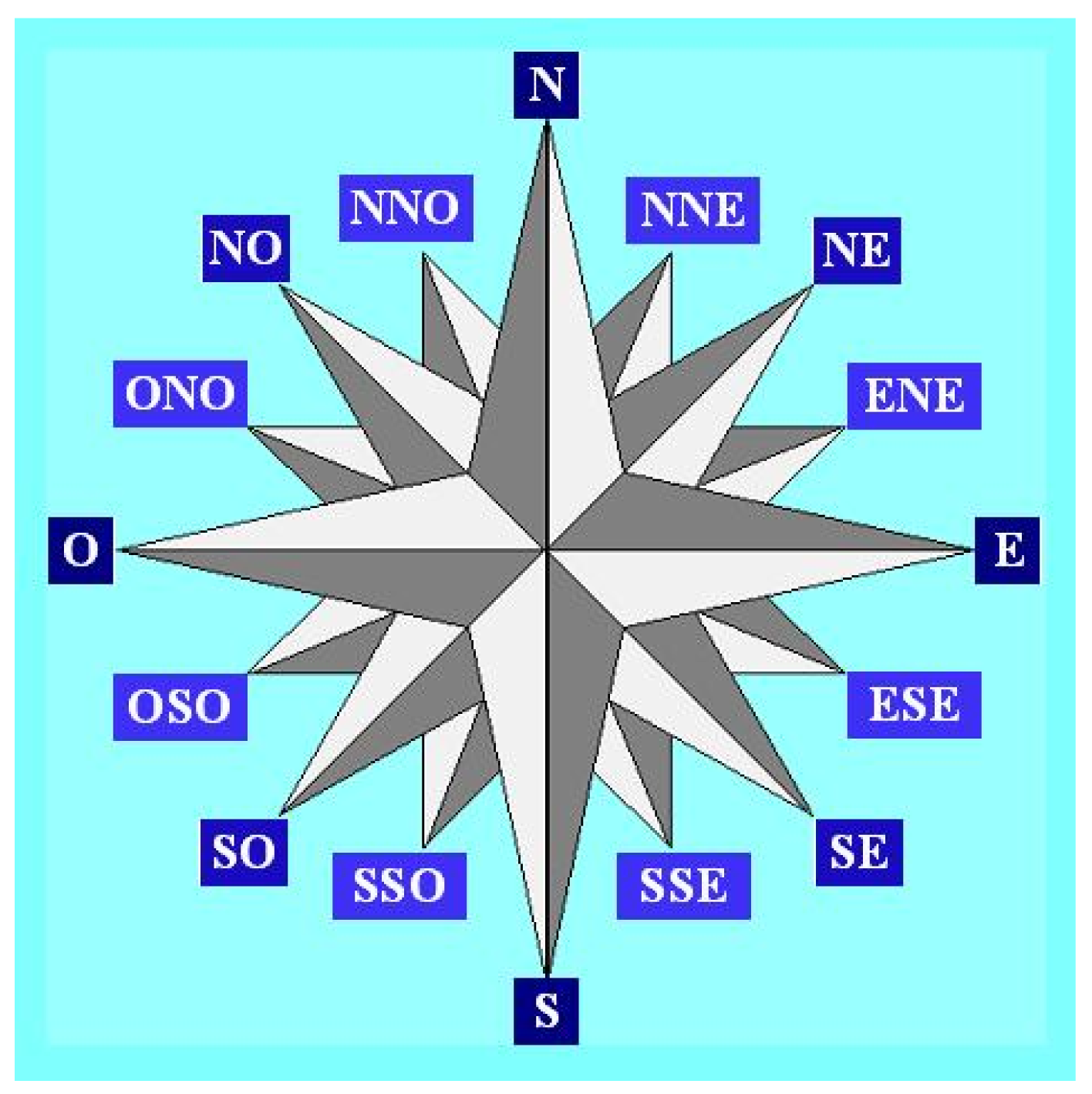
Five consecutive years (2002 to 2006) of hourly meteorological data have been used to investigate local meteorological conditions in Douala. Data are from the Douala international airport station, available at the National Direction of Meteorology. Due to the fact that Douala is 5 m above sea level in the littoral area of Cameroon and is located near the Atlantic Ocean, seasonal changes in rainfall are very significant. Each year, monthly rainfall average varies from 78.0 to 1215.0 (mm/month). Maximum precipitations occur between the months of July and September and are highly convective because the town is situated in the tropical zone. The period from December to February is the dry season. Temperatures range from 22 °C to 39 °C. Cloud cover is always about 6 to 7 Octas. Relative humidity has an average value of 70%. Wind speed is calm and the dominant direction of wind is around 220°N, from West according to the wind rose in the Figure 1. The wind rose is related to a circle which can be divided by 4, 8, 16 or 32 parts. As in the trigonometric circle, the main directions are: the North direction which corresponds to 0 or 360°, the East direction is 90°, the South is 180° and the West is 270°.
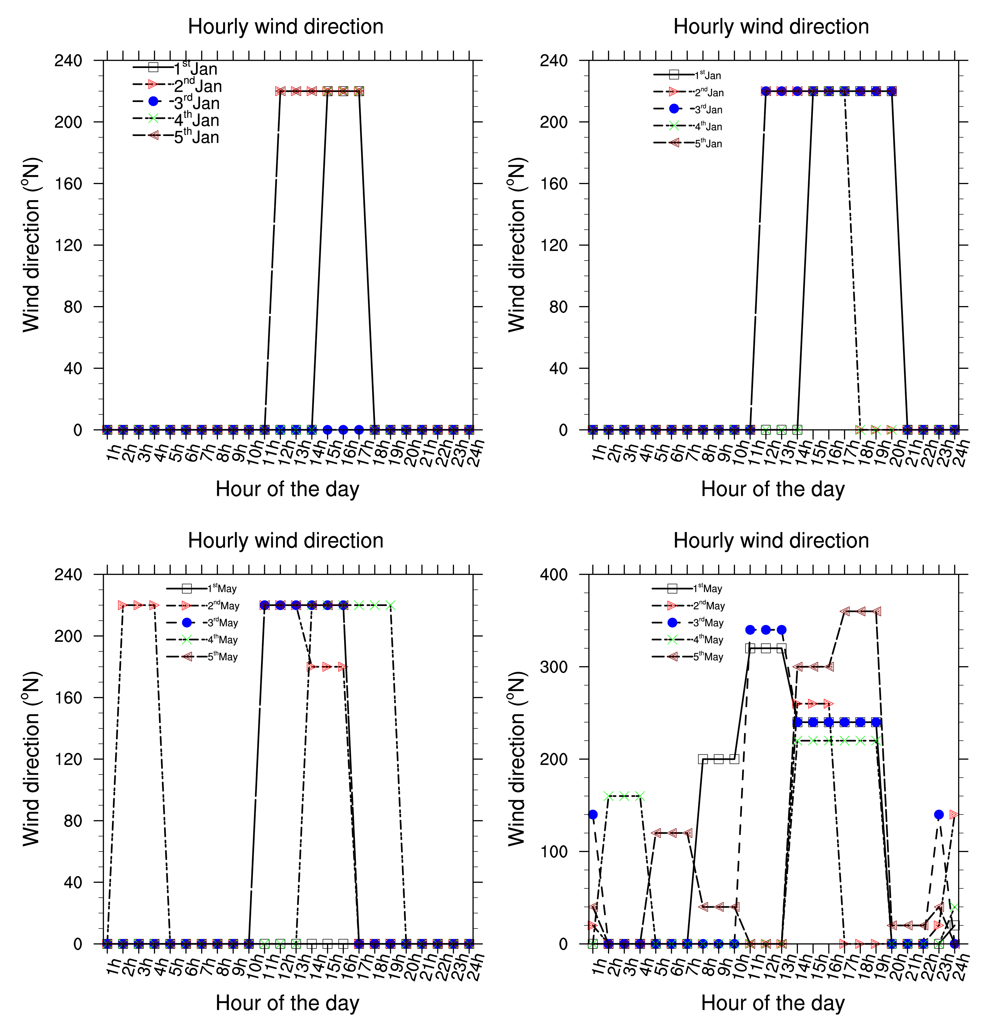
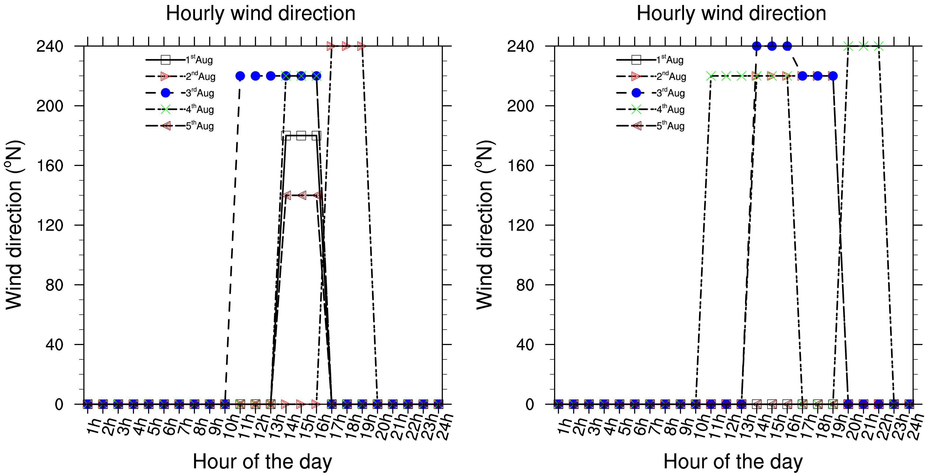
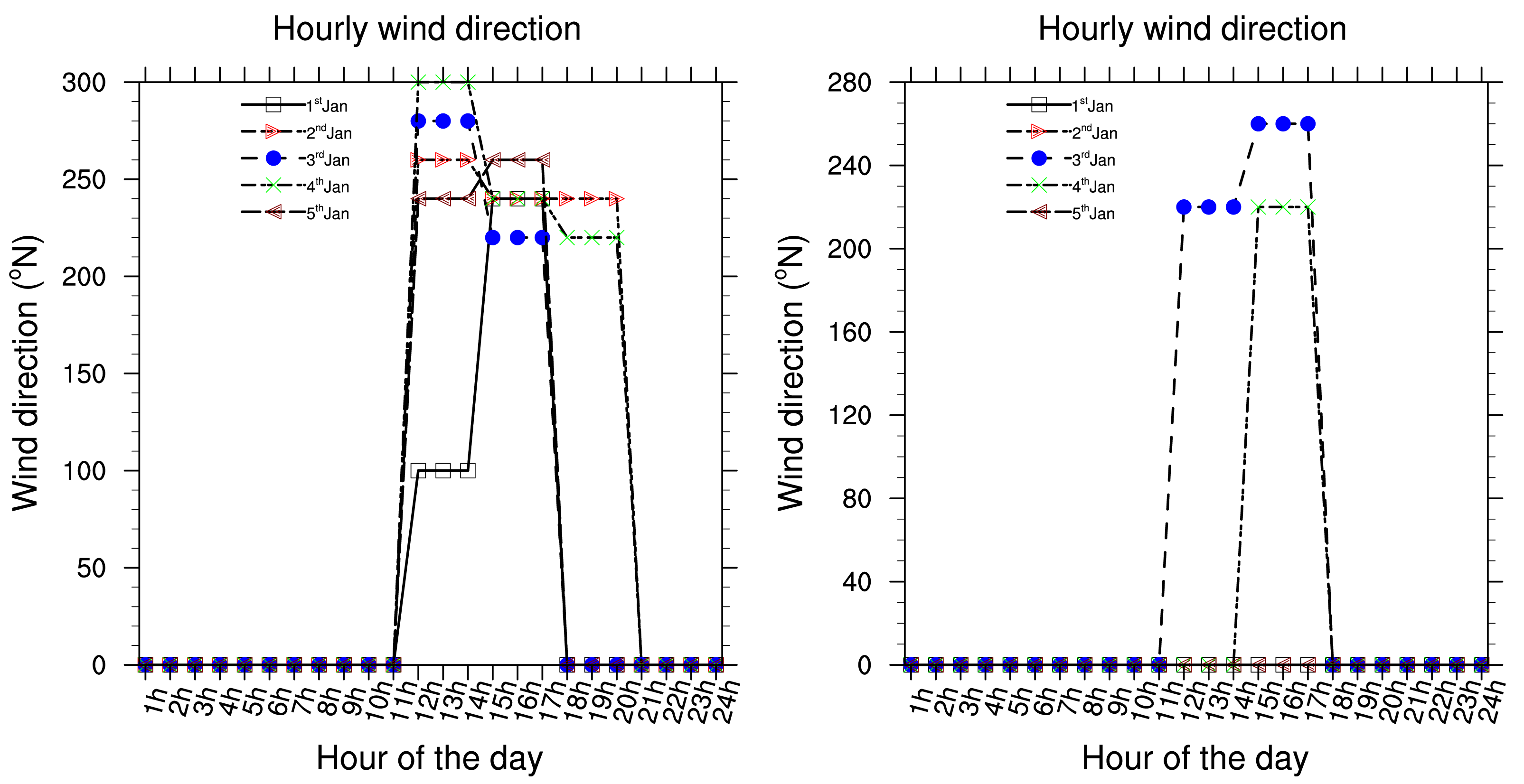
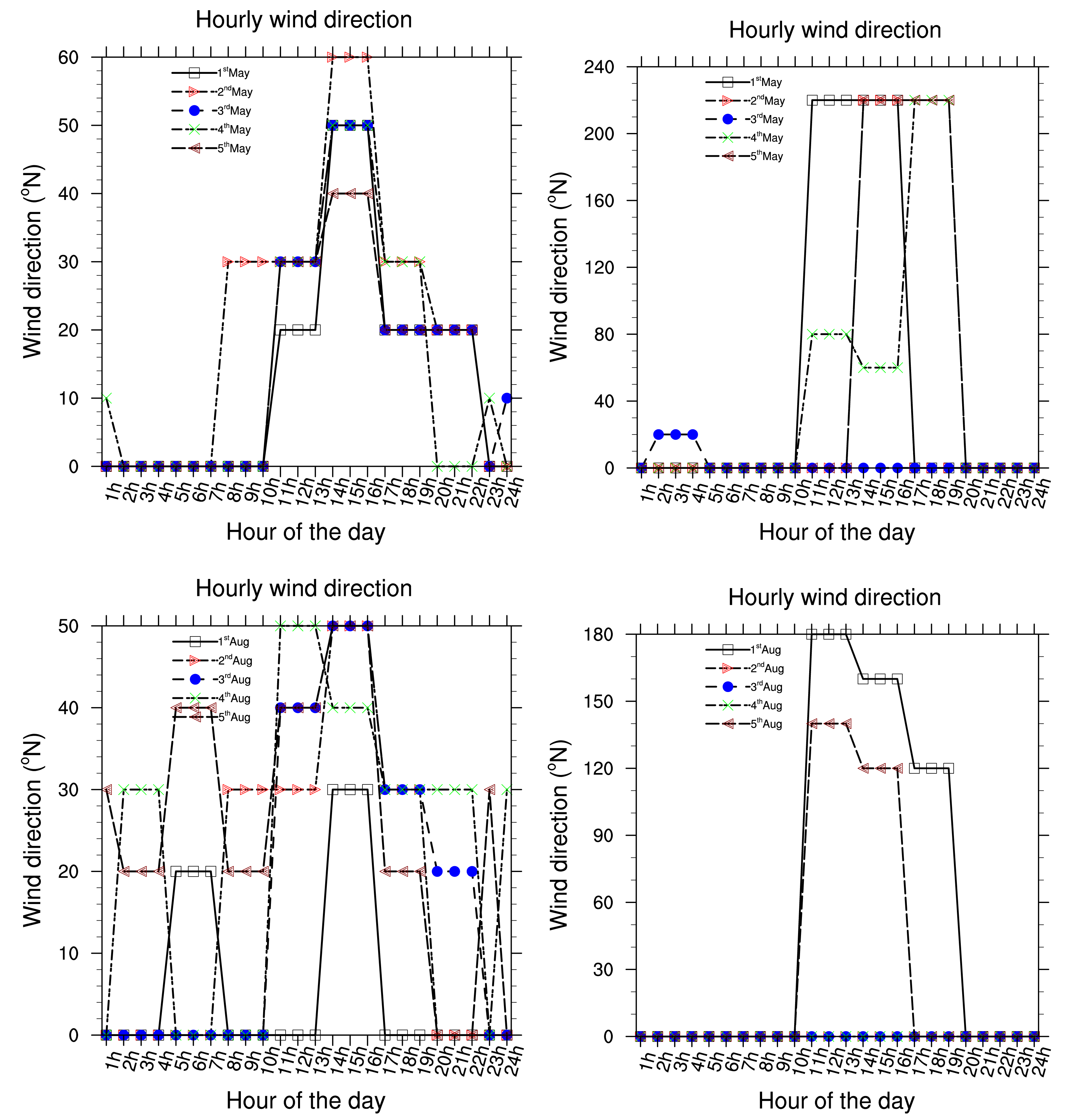
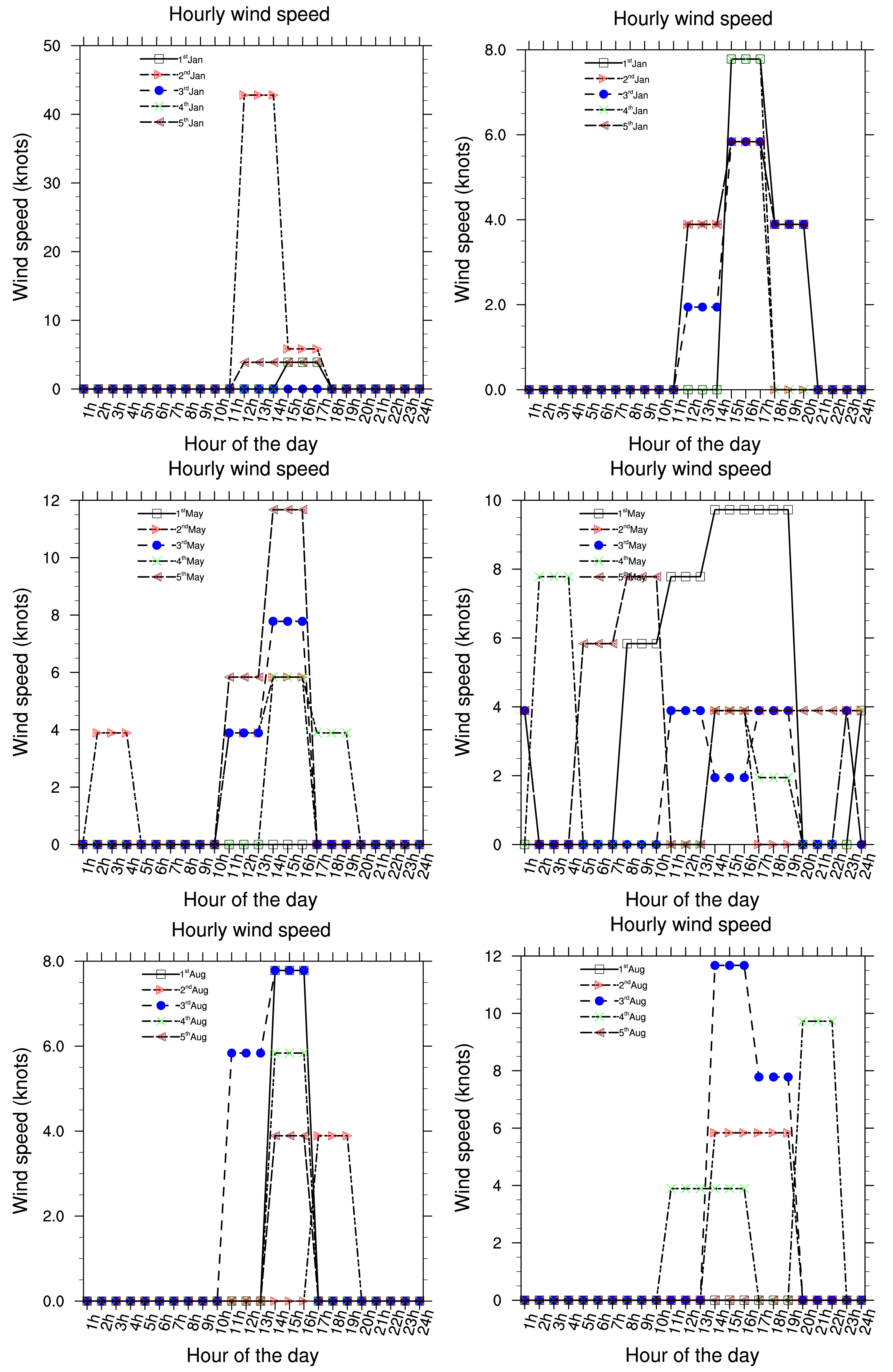
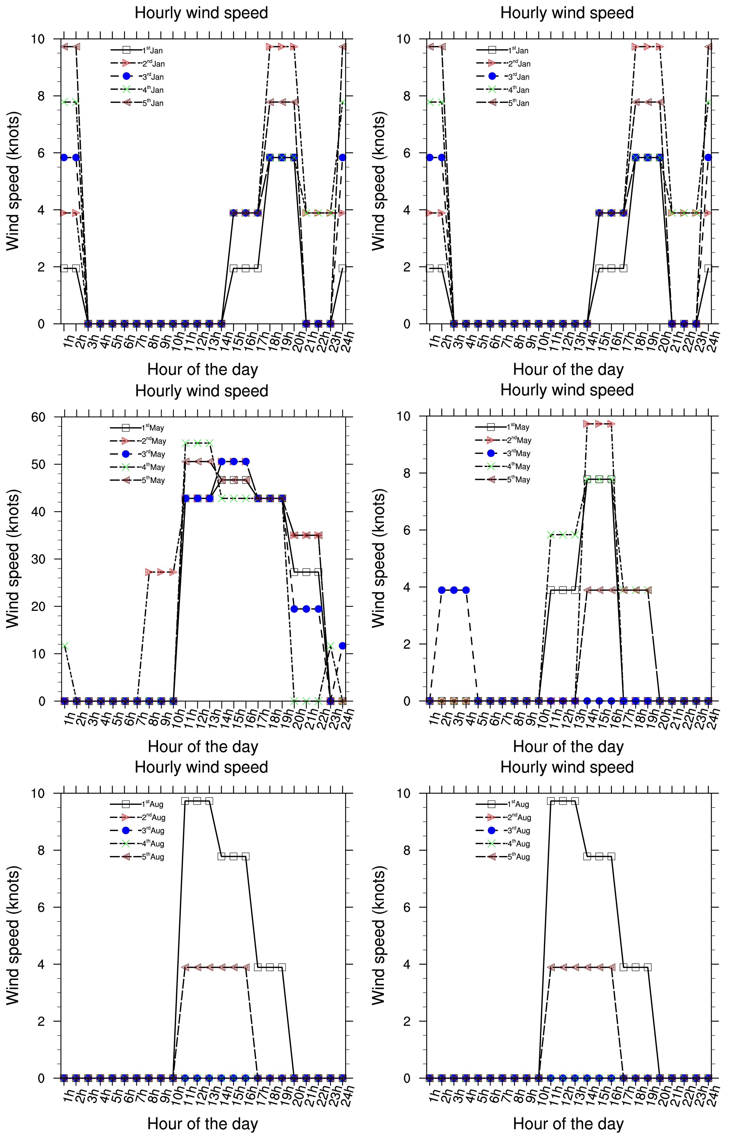
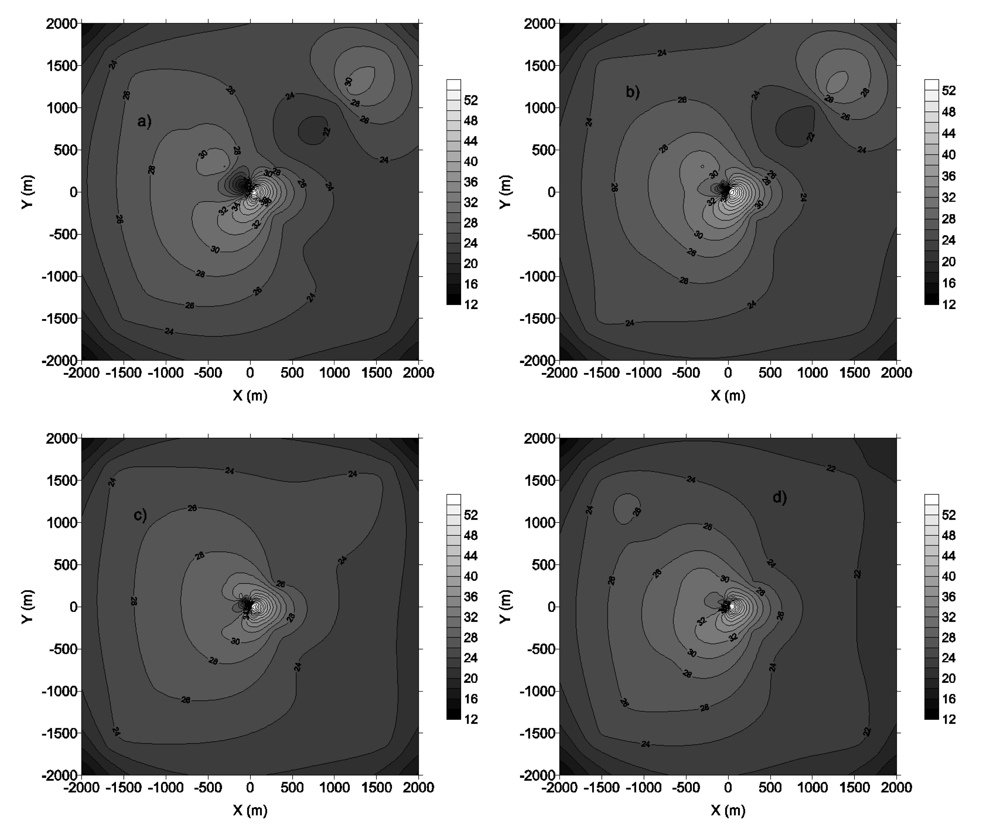
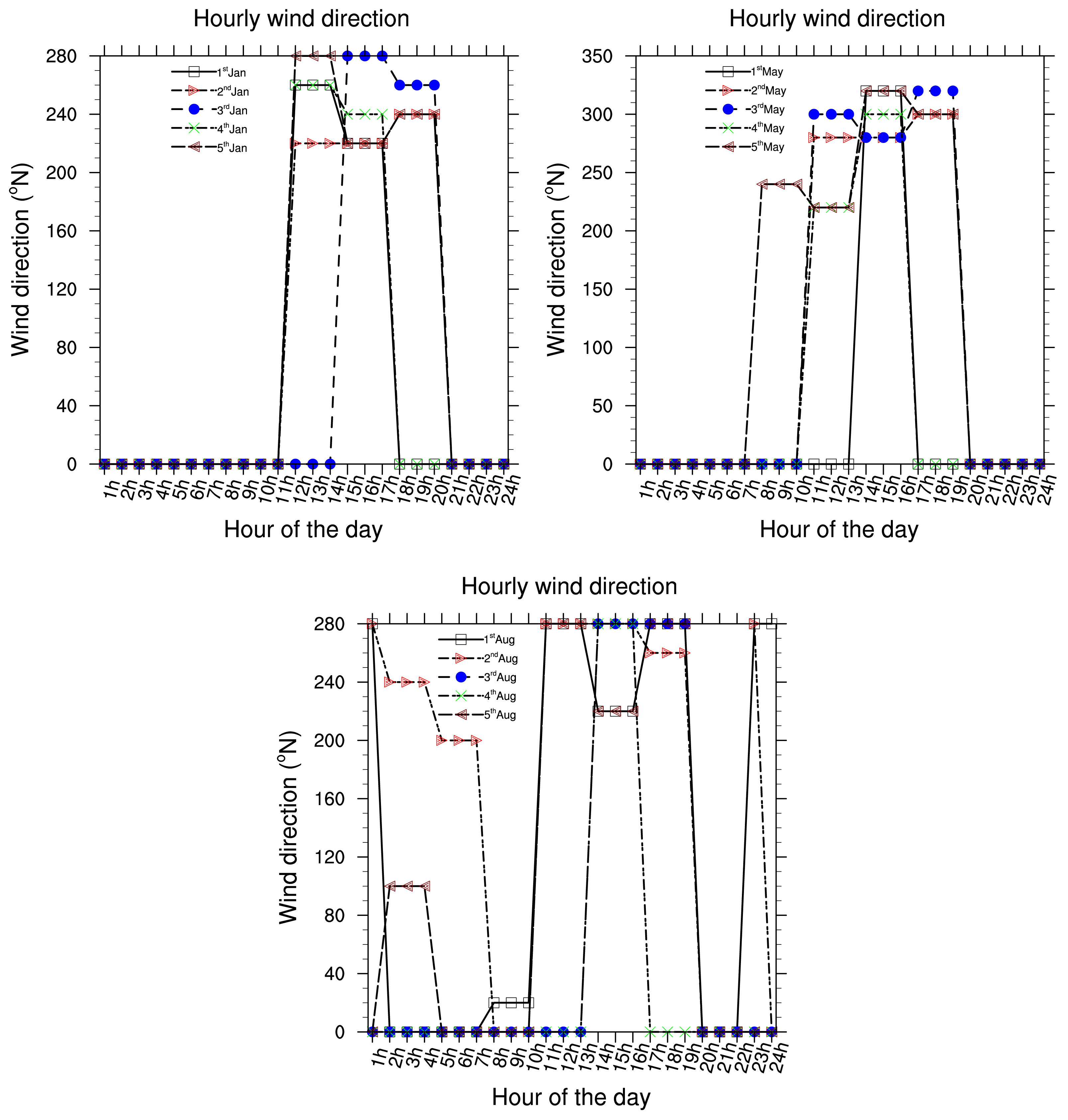
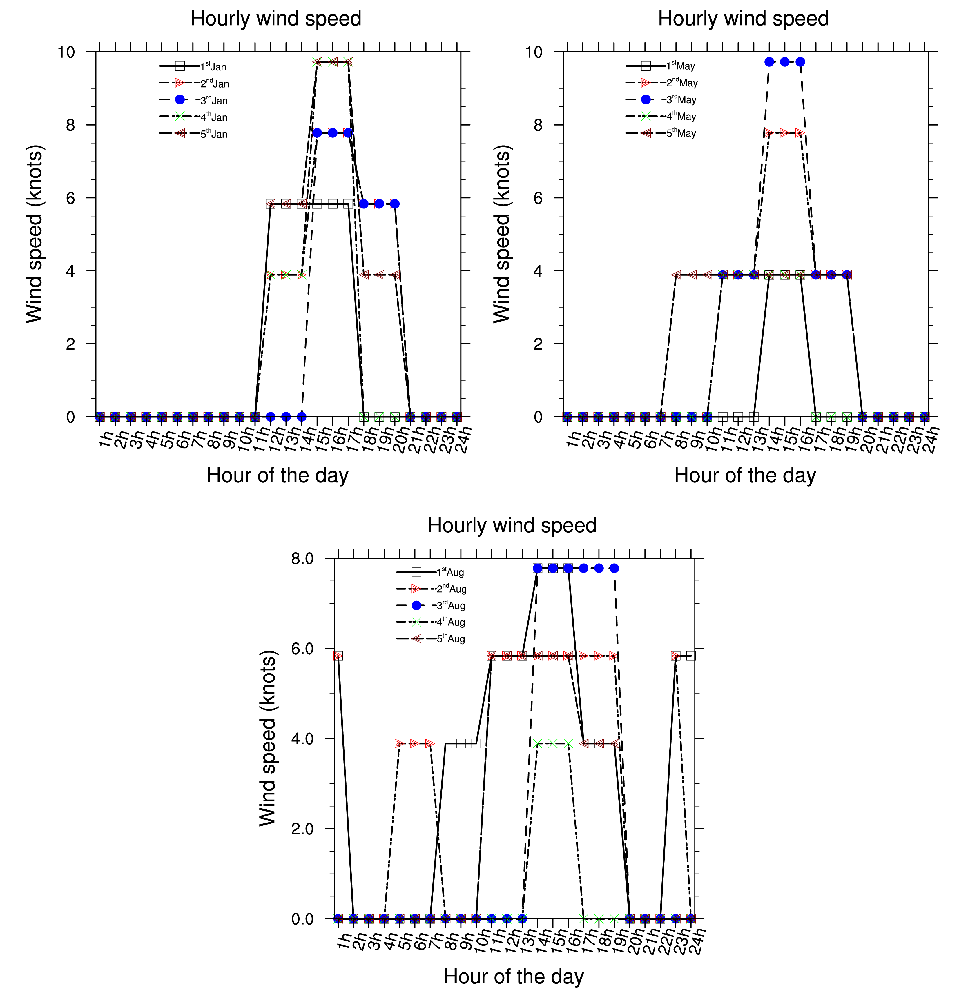
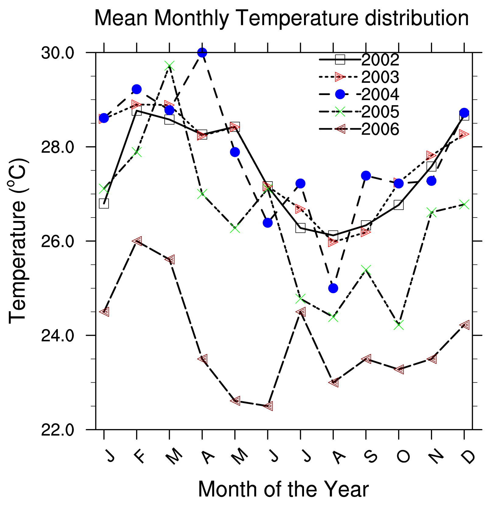
Presented below Figure 2–8 are the daily wind direction and speed for the first five days of the months of January, May and August for each year and the mean monthly average temperature for the years 2002 to 2006. We have selected the first five days of each month because daily variation in these data are not very important and the months have been selected to cover all the different season of Cameroon. We see from these figures that dominant wind direction is around 220°N to 270°N and occurs between 10 a.m. and 8 p.m., most frequently at 3 p.m. Winds are fairly strong between 9 a.m. and 8 p.m. and are calm for the remaining time. Maximum temperature occurs between February and April, while minimum occurs in August. One average, the year 2004 was the warmest and had registered the strongest wind speed with a value about 55 knots, while 2006 was the coldest one.
3.2. AERMOD Setup and Input Data
The model uses an urban dispersion, computes the main pollutant (Nitrogen Oxyde (NOx)) average concentration each 3 h, daily (24 h) and for all the period of study (5 years). The receptors (with heights of 50 m) are on a flat terrain and the concentration are evaluated on the ground. The output domain extend from the Logbaba power station (used by national company of electricity) to 2 km. Logbaba is a public quarter situated at the East site of Douala city. Furthermore, the NOx has been considered because it is released by almost of the entire industrial sites and vehicles and has a direct effects on human health. An unique source (stack) is considered, its characteristics are shown in Table 1.
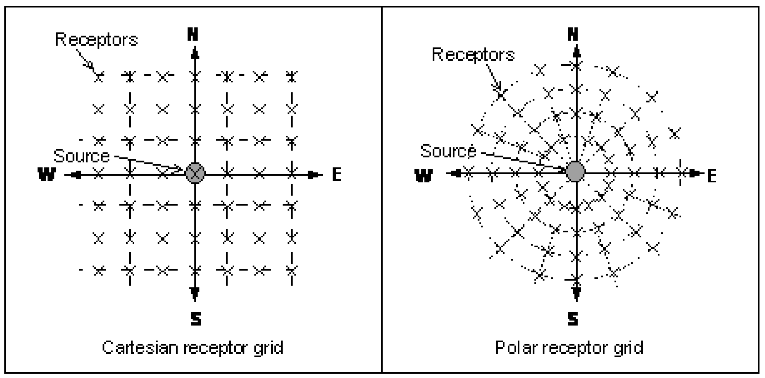
Concentrations are computed on 36 receptors located in a polar and a cartesian grid which spread from 0 to 2000 m to the source (Figure 9).
Meteorological data for the period 2002 to 2006 for the Douala international airport (4°N-9.7°E) have been used. Surface data are that have been taken at the Douala station. Upper air data are in the Forecast Systems Laboratory (FSL) format and are obtained from the National Oceanic and Atmospheric Administration (NOAA) free of charge. Whole description of these format are in AERMOD user's guide.
Dispersion modeling requires two types of data: surface and upper air data. Main surface data are from the National Weather Services (NWS) and consist at least of wind direction and speed, air temperature, cloud cover, the height of clouds, relative humidity and atmospheric pressure [13]. Upper air for the most cases describe the mixing height and are measured twice a day: the sounding of the 00 UTC and 12 UTC.
Typical values of albedo, Bowen ratio and roughness length are respectively 0.15, 2 and 1 m. Individual variation in each parameter is in adequation with vegetation and ground cover for the littoral zone of Cameroon. To test the effects of varying the land use parameters on the resulting modeled concentration patterns, albedo, Bowen ratio, and surface roughness length were varied over a range that one might expect to encounter in real life modeling situations. Table 2 summarizes all the runs performed.
4. Results and Discussion
4.1. Influence of Meteorological Fields in Terms of Distance from the Source to the Receptor
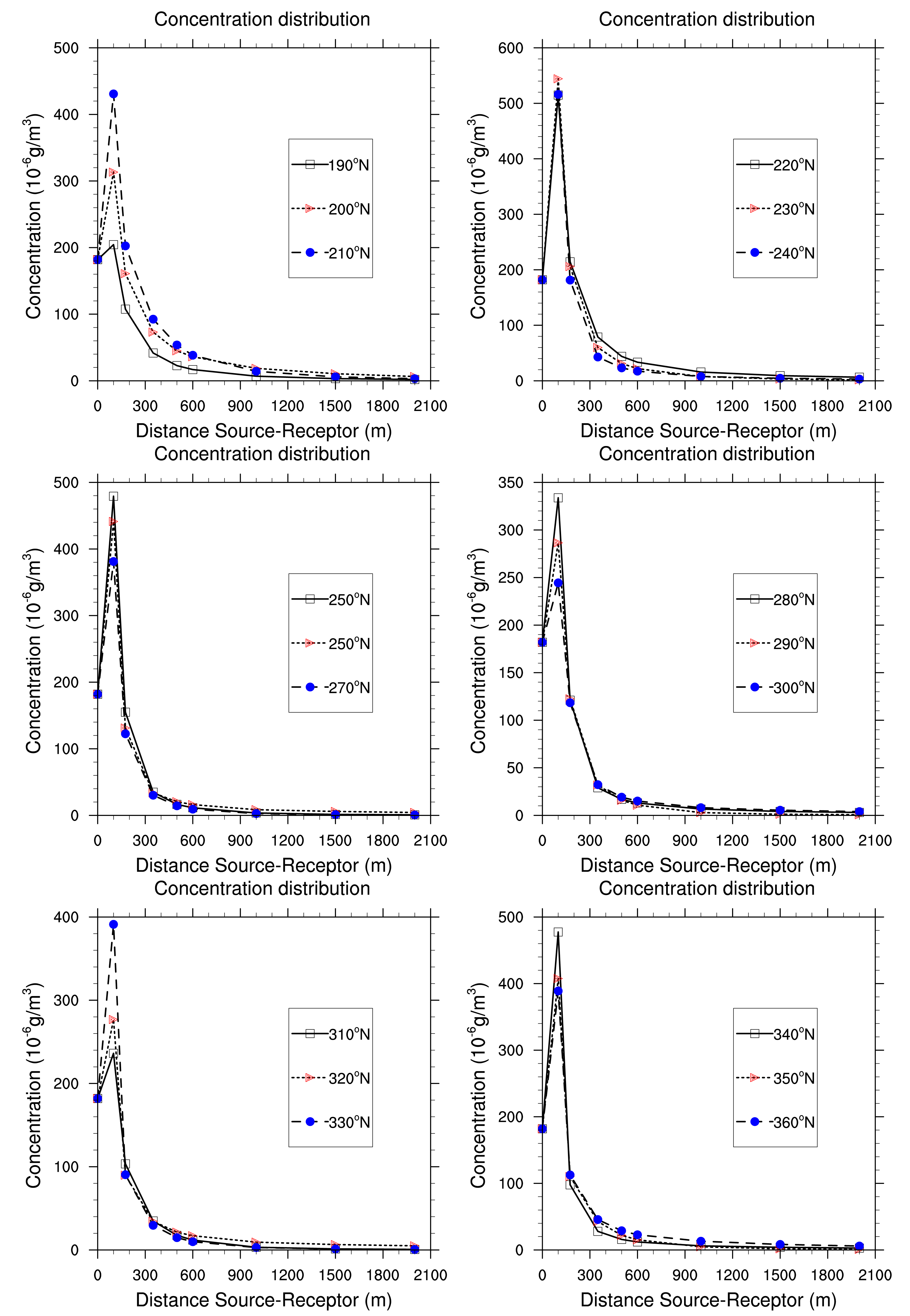
We use a polar grid so that we can analyse the distribution of the concentration when the plume rises away from the source. The values of albedo, roughness length and Bowen ratio are fixed to 0.15, 1 and 2 m respectively (the base case).
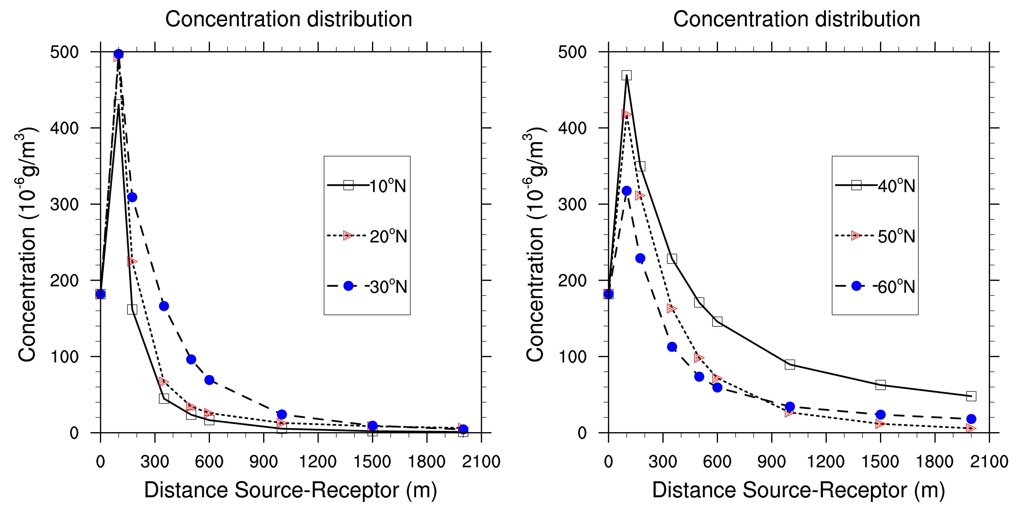
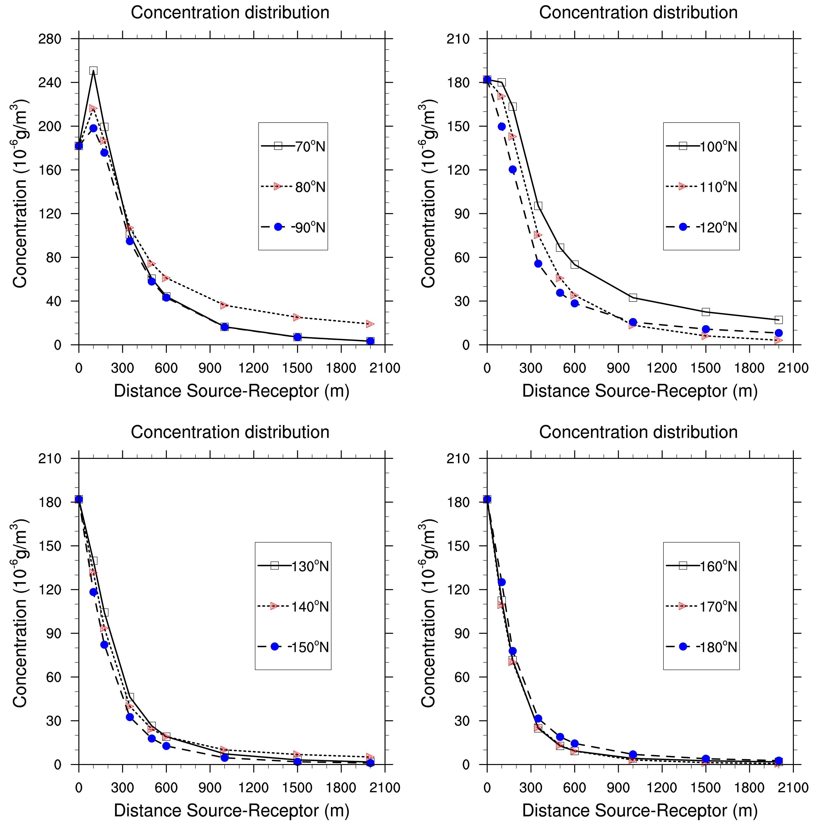
Figures 10 and 11 show a Gaussian distribution of air average concentration for all the period of study (5 years, i.e., 43,800 h). It appears that pollution increases gradually when pollutants are brought far from the source. The concentration reaches a threshold value of 497.16 μg/m3 generally around 100 or 150 m from the source. At this distance, the concentration begins to decrease progressively and vanishes. This case is encountered for the receptors situated at the North, North-East, South-West and North-West from the source. High concentration are due to low turbulence and low pressure (anticyclonics situations around the source. Such situations make the dispersion of pollutants slow. Thus, there is accumulation of pollutants. People and ecosystems around are exposed.
On the contrary, for receptors situated at the South-East sectors (100°N to 180°N), concentration are highest at the source, and decrease by dilution with ambient air to reach 1.41 μg/m3 at 1700 m from the source. Meteorological conditions are dominated by strong winds and low pressure (unstable atmosphere) which rapidly disperse air pollutants around the source. Atmospheric dispersion is then regulated in Planetary Boundary Layer (PBL) by advection transport through the average flux of wind and turbulence [26,27].
4.2. Influence of Albedo
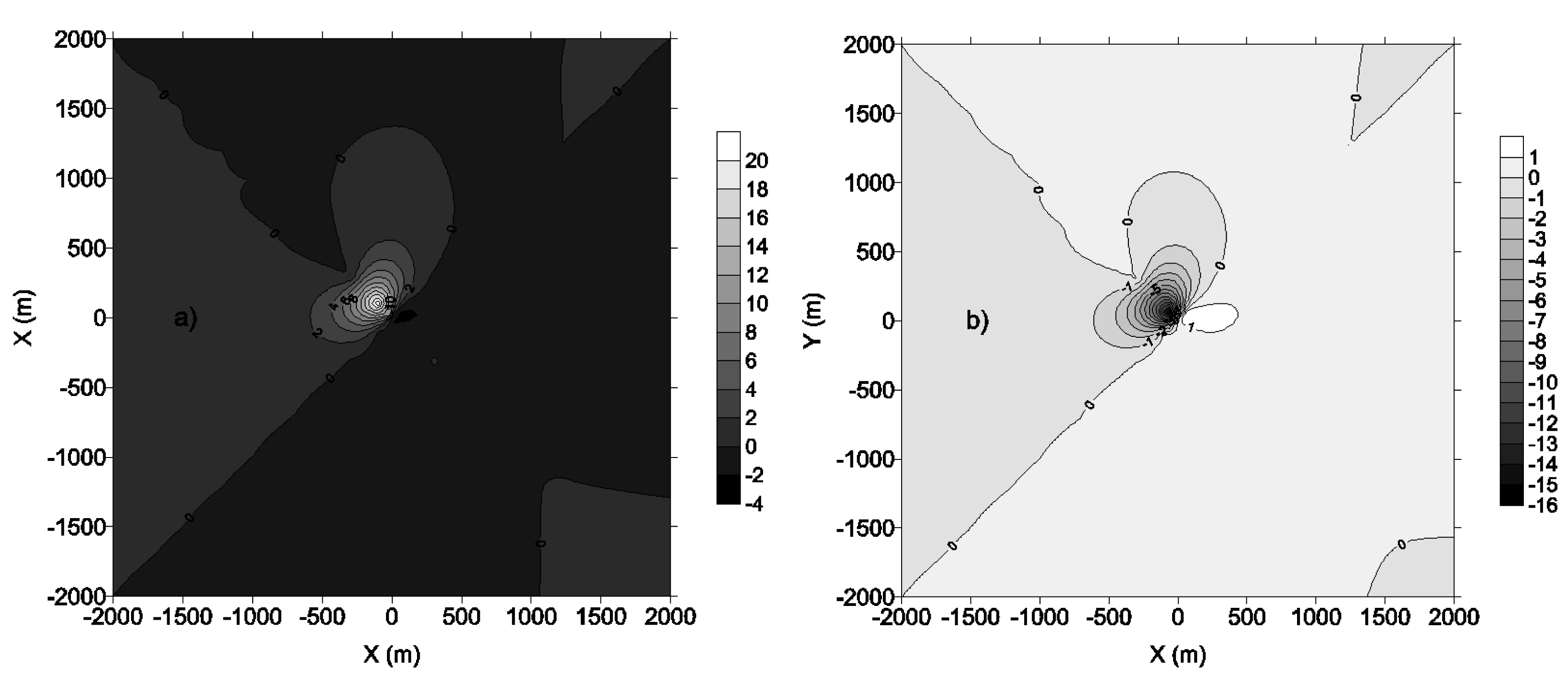
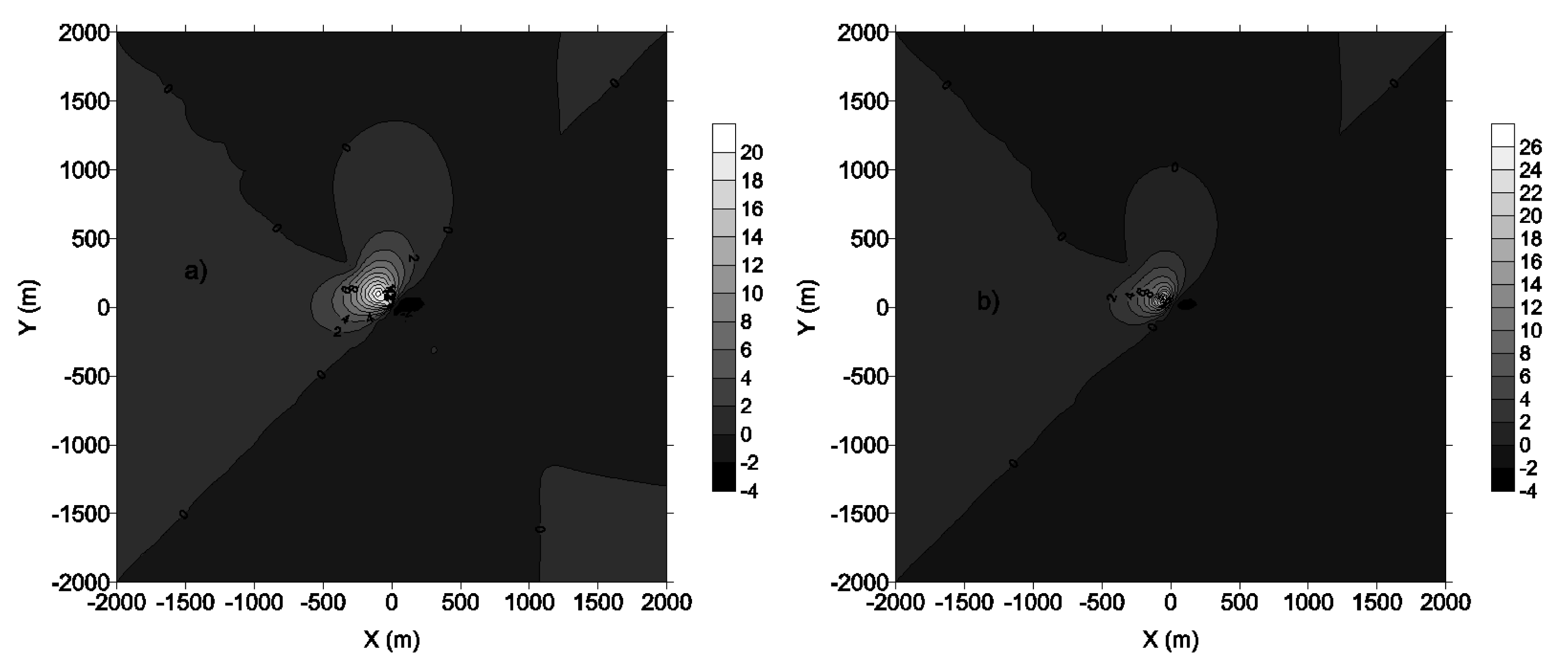
In order to study the sensitivity of AERMOD to changes in albedo, Bowen ratio and roughness length are fixed to 2 and 1 m respectively, successive values of 0.15 and 0.45 are given to the albedo (high albedo and base case). Equation (5) represents the relative variation of concentration patterns and highlights the sensitivity of concentration to albedo variation.
C0.45 and C0.15 are the concentration computed with an albedo value of 0.45 and 0.15 respectively.
Figure 12a,b represent the 3 h first and second highest concentration whereas Figure 12c,d are the 24 h first and second highest concentration.
It comes out that, sites located at the same distance from the source are not equally exposed to pollution. Contour lines are confined around the source and are not circular due to wind flow, turbulence and atmospheric stability. Tables 3 and 4 reveal that highest concentration occurred most at the time in the afternoon for 3 h averaging concentration and the night for 24 h concentration when high pressure and temperature inversion occur. In the case of temperature inversion, pollutants are held back near the ground. It happens for example in front of warm front (atmospheric perturbation) due to the fact that the Douala city is located by the sea. Cool air is held back in warm air's layer which reacts as a cover, thus pollutants of cool layer do not disperse and dwell concentrated at the ground. Very near to the source, dominant winds are from East and North-West. Around 350 m from the source, the wind is from South-West.
Dispersion and wind appear to be linked by the relation:
The greater the soil's albedo, the thicker and the cooler the air masses near the ground. An increase in albedo leads to a decrease in the sensible heat flux, the friction velocity, the Monin–Obukhov length, the convective and the mechanic mixing heights. And yet the potential rate temperature increases. The first highest 3 hour averaging time concentration patterns (Figure 12a) behave differently from the others in Figure 12. Figures 12b–d reveal a decrease in concentration patterns of about 16%, 24% and 11% respectively, while Figure 12a shows an increase in the concentration patterns. This may seem contradictory, but a close look at the results reveals a decrease in the air concentration when albedo increases. The effects of changes in albedo are to be considered for the second highest concentration which is the criterion for most regulatory standards in the United states [6].
4.3. Influence of Roughness Length
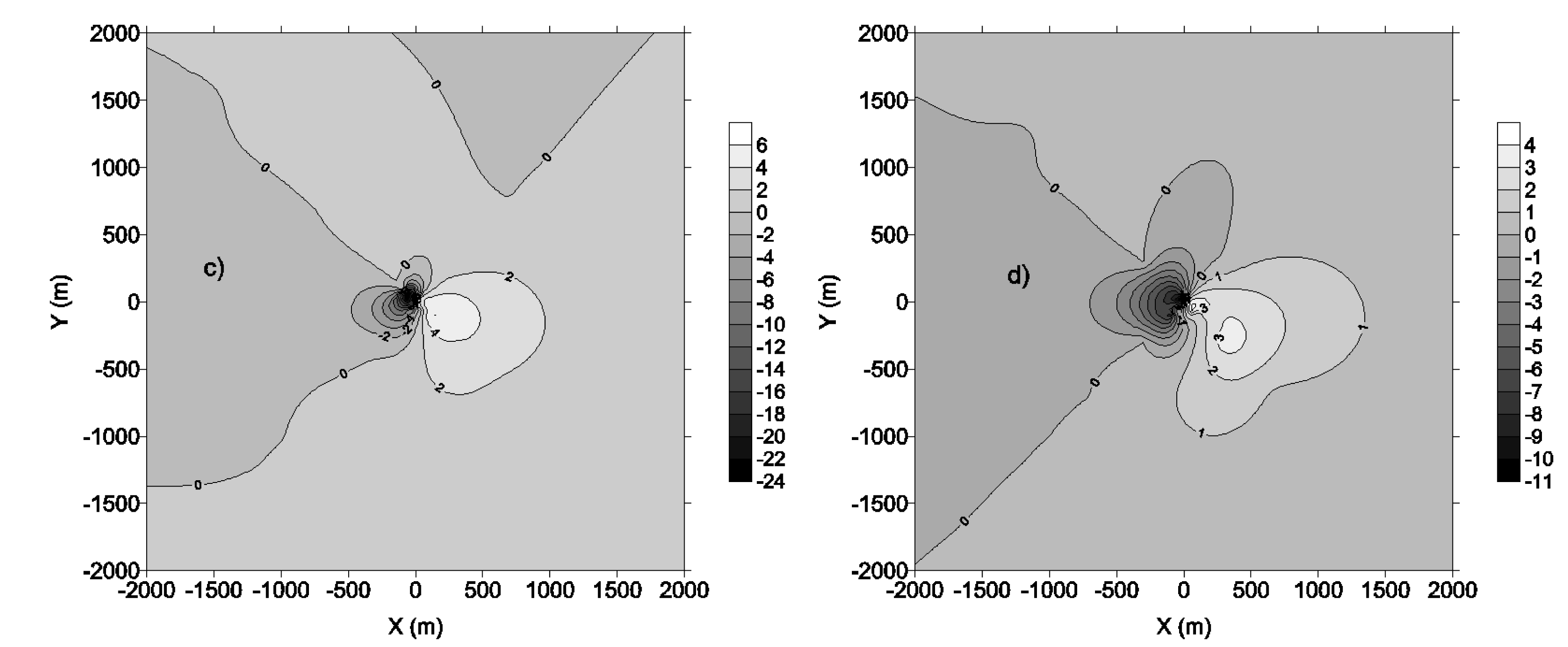
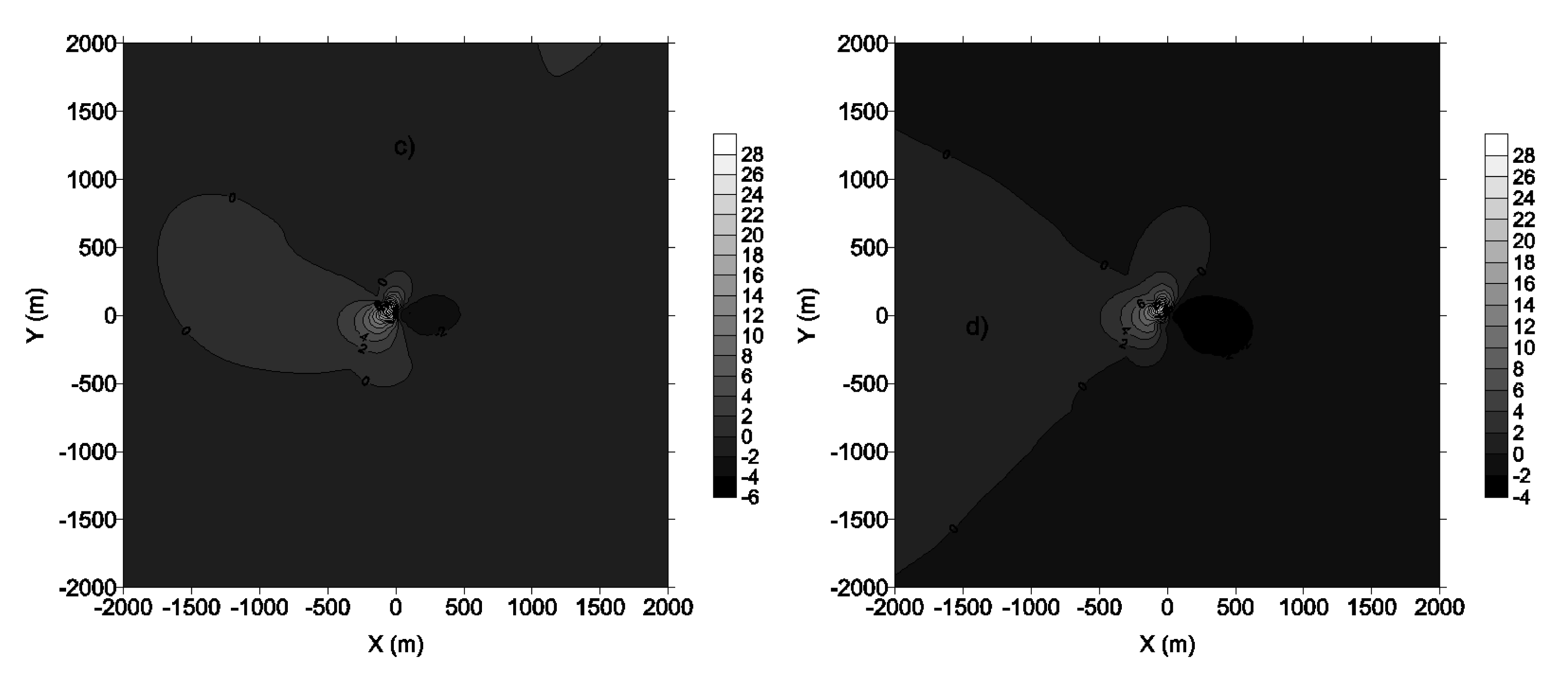
Let's now turn to roughness length values of 0.3 and 1 m (low roughness length and base case), albedo and Bowen ratio are fixed to 0.15 and 2. Using the Equation (7), where C0.3 and C1 are the concentration computed with a roughness length value of 0.3 and 1m respectively, we obtain the figures below where
Figures 13a,b represent the 3 h first and second highest concentration and Figure 13c,d are the 24 h first and second highest concentration.
Concentration fluctuations in time and space are always the fact of atmospheric pressure, wind and temperature inversion. The wind from South remains dominant. The presence of buildings and vegetation increases the roughness length of soil. For unstable conditions, i.e., where convective turbulence dominates, the roughness length causes the growth of the vertical dispersion of the plume and changes the vertical profile of wind speed on the higher grounds due to the growth of mechanical turbulence caused by the movement of air above the ground [28]. The effects of variations in roughness length are quiet remarkable when one moves away from the source; these effects are greatly dependent on the nature of the source. Thus the effects of changes in roughness length are sharper for discharges into contact or near the soil surface than for the high chimneys.
We noticed that the sensible heat flux, the potential temperature gradient and convective mixing height have not changed. The friction velocity and the mechanical mixing height have increased and then affects significantly the air quality. Concentrations have greatly diminished with the increase in roughness length and reached the rate of 52% (Figure 13). The roughness length greatly influences the dispersion because it has direct effect on the pollutants transport and is the height at which the average horizontal wind speed is zero.
4.4. Influence of Bowen Ratio
The Bowen ratio is an indicator of amount of moisture on the earth's surface. When we make it vary, according to Equation (8),
All the input parameters generated by AERMET have increased, with the exception of gradient of potential temperature which remains constant. We notice that when the soil is wetter, that is to say when the Bowen ratio increases from 0.5 to 2 (low Bowen ratio and base case), we observe an increase in the ground concentration. Figure 14 shows that the increase reaches the amount of 20% in relative variation. A wet soil is permeable, thus absorbs substances in contact with it. It influence on the pollutants concentration is somewhat similar to that of the albedo.
5. Model Outputs Verification
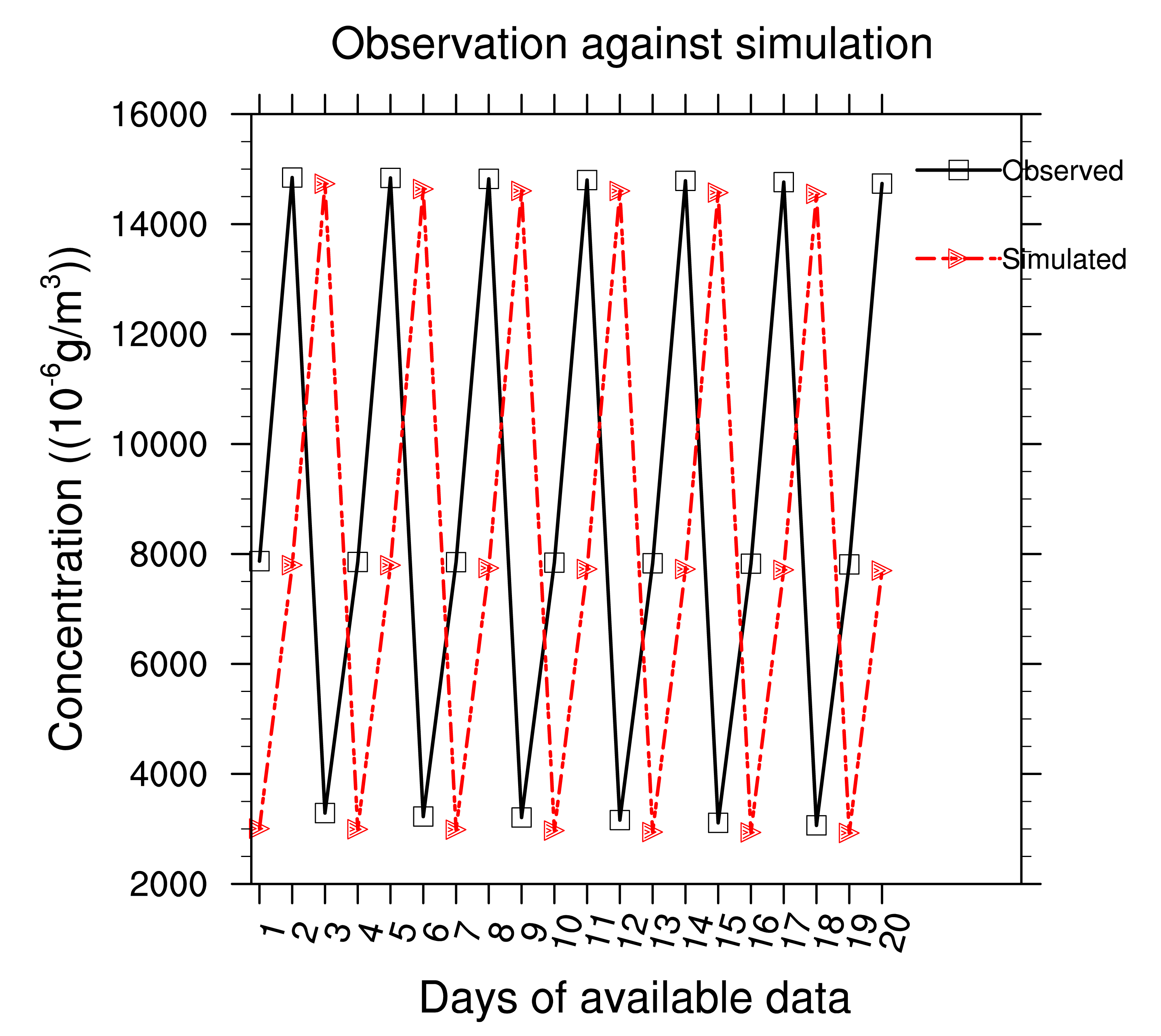
Daily in situ observations data have been collected from the Cameroonian's Ministry of territorial administration and decentralisation, direction of civilian protection. Since AERMOD just produces highest mean concentrations for the a given period (3 h for example) and indicates the dates at which they occur, we have collected data corresponding to the first 20 maximum average concentration values for a period of 24 h. The outputs discussed here is the base case presented in the Table 2. Figure 15 represents the observed concentration of NOx against simulated. The model underestimates the simulated NOx concentration. For the twenty data we recorded, the Root Mean Square Error (RMSE) is about 2.91. It comes out that the model does not reproduce satisfactory the real case pollution over Douala. This is due to lack of meteorological data.
6. Conclusions
The sensitivity of the AERMOD dispersion model to atmospheric fields and land use parameters has been investigated. We have shown that calm winds and anticyclonic conditions are not favorable to atmospheric dispersion. Air temperature and solar radiation play an important role: Cool air conditions decrease the volatility of some gases. Air concentration of primary pollutants are highest near the sources, and tend to decrease far from the source by dilution with ambient air [29]. Also, pollutants concentration decreases exponentially with respect to the inverse of distance from the source. The diurnal variation of albedo, Bowen ratio and roughness length are modulated by the solar radiation and energy budget at the top of atmosphere. An increase in albedo or roughness length leads to a decrease in pollutants concentration, but more significantly for the roughness length. Whereas an increase in the Bowen ratio increases pollutants concentration. Globally, albedo and Bowen ratio have less effects on concentration patterns than the roughness length, this is to be expected since albedo and Bowen ratio only affect the retention of incoming solar radiation, and therefore have no effect at night or just during convective conditions. Moving from 3 h to 24 h and to 5 years, pollutants concentration has significantly decreased. Thus, we recommend Cameroonian authority to move industrial sites from West site of Douala (Bonaberi industrial area, a popular quater of Douala city) to Nyala area (East site of Douala and not yet so more populated). Minimization (reduction) of environmental impacts are prior to a choice of land with a high roughness length and albedo. Thus, preliminary studies, meaning that an analysing of the land properties should be done before implanting industrial sites.


| Stack Height | Stack Diameter | Gas Temperature | Gas Velocity | Emission Rate |
|---|---|---|---|---|
| 20 m | 0.6 m | 340 K | 19.7 m/s | 24.20 g/s |
| Scenario | Albedo | Bowen Ratio | Roughness Length |
|---|---|---|---|
| Base case | 0.15 | 2 | 1m |
| High albedo | 0.45 | 2 | 1m |
| Low Bowen ratio | 0.15 | 0.5 | 1m |
| Low roughness length | 0.15 | 2 | 0.3 m |
| Rank | Concentration (μg/m3) | Date (YYMMDDHH) | XR | YR |
|---|---|---|---|---|
| 1 | 13903.50 | 05020915 | −50.00 | 86.60 |
| 2 | 13064.63 | 05020915 | −34.20 | 93.97 |
| 3 | 10395.20 | 05071715 | −34.20 | 93.97 |
| 4 | 9925.95 | 03122215 | −34.20 | 93.97 |
| 5 | 9873.13 | 03061815 | −34.20 | 93.97 |
| 6 | 9635.77 | 02032618 | −34.20 | 93.97 |
| 7 | 9565.95 | 05071715 | −50.00 | 86.60 |
| 8 | 9545.34 | 02031915 | −34.20 | 93.97 |
| 9 | 9480.76 | 06060215 | −34.20 | −93.97 |
| 10 | 9479.71 | 03053115 | −34.20 | 93.97 |
| Rank | Concentration (μg/m3) | Date (YYMMDDHH) | XR | YR |
|---|---|---|---|---|
| 1 | 4515.59 | 05020924 | −34.20 | 93.97 |
| 2 | 4432.76 | 03051424 | −98.48 | 17.36 |
| 3 | 4086.23 | 05020924 | −50.00 | 86.60 |
| 4 | 4067.97 | 03051424 | −93.97 | 34.20 |
| 5 | 3839.21 | 03051424 | −100.00 | 0.00 |
| 6 | 3321.96 | 03040524 | −76.60 | −64.28 |
| 7 | 3299.34 | 03040524 | −64.28 | −76.60 |
| 8 | 3288.00 | 03041424 | −98.48 | 17.36 |
| 9 | 3225.17 | 05071724 | −34.20 | 93.97 |
| 10 | 3206.93 | 05032524 | −100.00 | 0.00 |
Acknowledgments
The model has been provided free of charge by US/EPA. Surface data were obtained from the Douala international airport and upper air data from the NOAA (FSL data). Surfer and NCL software were used for visualization. Special thanks to Pr Olivier TALAGRAND of Laboratoire de Météorologie Dynamique (LMD), Paris, France for providing us the financial support for the payment of English Editing Fees.
References
- André, J.C.; Royal, J.F. Les fluctuations à court terme du climat et l'interprétation des observations récentes en termes d'effet de serre (Short-term climatic fluctuations and the interpréation of réent observations in terms of greenhouse effect). Comptes Rendus de I'Acadéie des Sciences (Series IIA-Earth Planet. Sci.) 1999, 28, 211–272. [Google Scholar]
- Sportisse, B. Modélisation de la Pollution Atmosphérique; Centre d'Enseignement et de Recherche en Environnement Atmosphérique, Laboratoire Commun EDF R&D-ENPC: Paris, France, 2004. [Google Scholar]
- Uliasz, M. The atmospheric mesocale dispersion modeling system. J. Appl. Meteorol. 1993, 32, 139–149. [Google Scholar]
- Zou, B.; Zhan, F.B.; Wilson, J.G.; Zeng, Y. Performance of AERMOD at different time scales. Simul. Model. Pract. Theory 2010, 18, 612–623. [Google Scholar]
- USEPA/AMS. User's Guide for the Idustrial Source Complex Dispersion Models, Version 3; USEPA, Office of Air Quality Planning and Standars, Emissions Monitiring and Analysis, Division: Research Triangle Park, NC, USA, 1995; p. 390. [Google Scholar]
- USEPA/AMS. User's Guide for the AMS/USEPA Regulatory Model; EPA-454/B-03-001; USEPA, Office of Air Quality Planning and Standars, Emissions Monitiring and Analysis, Division: Research Triangle Park, NC, USA, 2004; p. 216. [Google Scholar]
- Weil, J.C. Updating the ISC Modelthrough AERMIC. Proceedings of the 85th Annual Meeting of Air and Waste Management Association, Air and Waste Management Association, Kansas City, PA, USA, 21–26 June 1992.
- Bowers, J.F.; Anderson, A.J. An Evaluation Study for the Industrial Source Complex (ISC) Dispersion Model; Report EPA-450/4-81-002; NTIS PB81-176539; United States Environmental Protection Agency Office of Air Quality Planning and Standards: Research Triangle Park, NC, USA, 1981. [Google Scholar]
- USEPA/AMS. AERMOD: Latest Features and Evaluation Results; EPA-454/R-03-003; USEPA, Office of Air Quality Planning and Standars, Emissions Monitiring and Analysis, Division: Research Triangle Park, NC, USA, 2003. [Google Scholar]
- Vondou, A.D.; Nzeukou, A.; Mkankam, K. Diurnal cycle of convective activity over the West of Central Africa based on meteosat images. Int. J. Appl. Earth Obs. Geoinf. 2010, 12, S58–S62. [Google Scholar]
- Ministry of Public Health. Urban Pollution Expossure in The Main Capital Cities of Cameroon: Yaounde and Douala; Yaounde, Republic of Cameroon, 2008. [Google Scholar]
- Dabberdt, W.F.; Carroll, M.A.; Baumgardner, D.; Carmichael, G.; Cohen, R.; Dye, T.; Ellis, J.; Grell, G.; Grimmond, S.; Hanna, S.; et al. Meteorological research needs for improved air quality forecasting report of the 11th prospectus development team of the US weather research program. Bull. Am. Meteorol. Soc. 2004, 85, 563–586. [Google Scholar]
- USEPA/AMS. User's Guide for the AERMOD Meteorological Preprocessor; EPA-454/B-03-001; USEPA, Office of Air Quality Planning and Standars, Emissions Monitiring and Analysis, Division: Research Triangle Park, NC, USA, 1998; p. 273. [Google Scholar]
- Van Ulden, A.; Holslag, A.M. Estimation of atmospheric boundary layer parameters for diffusion applications. J. Appl. Meteorol. 1985, 24, 1196–1207. [Google Scholar]
- Hernández, E.; Martín, F.; Valero, F. State-space modeling of atmospheric pollution. J. Appl. Meteorol. 1991, 30, 793–811. [Google Scholar]
- Couillet, J.C. Méthode Pour l'Evaluation et la Prévention des Risques Accidentels; INERIS, Ministère de l'Ecologie et du Développement Durable, Direction de Risques Accidentels: Oise, France, 2002; p. 61. [Google Scholar]
- McCaughey, J.H. A reversing temperature-difference measurement system for bowen-ratio determination. Bound.-Layer Meteorol. 1981, 21, 47–55. [Google Scholar]
- Rao, K.S.; Wyngaard, J.C.; Cote, O.R. The structure of the two-dimensional internal boundary layer over a sudden change of surface roughness. J. Atmos. Sci. 1973, 31, 738–746. [Google Scholar]
- Panofsky, H.A.; Dutton, J.A. Atmospheric Turbulence: Models and Methods for Engineering Applications; John Wiley & Sons: New York, NY, USA, 1984; p. 397. [Google Scholar]
- Oke, T.R. Boundary Layer Climates; John Willey & Sons: New York, NY, USA, 1978. [Google Scholar]
- Venkatram, A. Estimating the Monin-Obukhov length in the Stable Boundary Layer for dispersion calculations. Boud.-Layer Meteorol. 1980, 19, 481–485. [Google Scholar]
- Carson, D.J. The development of dry inversion-capped convectively unstable boundary layer. Q. J. R. Meteorol. Soc. 1988, 099, 450–467. [Google Scholar]
- Weil, J.C.; Brower, R.P. Estimating Convective Boundary Layer Parameters for Diffusion Applications; Draft Report Prepared by the Environment Center, Martin Mariette Corp for the State of Maryland: Baltimore, MD, USA, 1983. [Google Scholar]
- Arguin, L.; Gagnon, C. Modélisation Niveau 2 de la Dispersion Atmosphérique de Biogaz. Lieu D'enfouissement Sanitaire de Val-d'Or; 270123-140-ENV-001 00; MRC De Vallée-De-l'Or, Environnement et Infrastructures, N/Réf.: Québec, Canada, 2003; p. 25. [Google Scholar]
- Leduc, R. Guide de la Modélisation de la Dispersion Atmosphérique; Direction du milieu atmosphérique, Ministére de l'environnement et de la faune: Quebec, Canada, 1998. [Google Scholar]
- Gifford, F.A., Jr. Turbulent diffusion typing shemes. A review. Nucl. Saf. 1976, 17, 68–86. [Google Scholar]
- Pasquill, F.; Smith, F.B. Atmospheric Diffusion, 3rd ed.; Ellis Horwood: Chichester, UK, 1983. [Google Scholar]
- New Zealand Ministry for the Environment, M.M.T.T. Good Practice Guide for Atmospheric Dispersion Modeling; Number 522; National Institute of Water and Atmospheric Research: Wellington, New Zealand, 2004. [Google Scholar]
- Khalaifi, A.; Dahech, S.; Ionescu, A.; Beltrando, G.; Candau, Y. Modélisation de La Dispersion des Polluants Atmosphériques an Situation Anticyclonique Estivale Exemple de La Ville de Afax. Proceedings of XVIIIme Colloque de l'Association Internationale de Climatologie, Genoa, Italy, 7–11 September 2005; pp. 43–47.
© 2011 by the authors; licensee MDPI, Basel, Switzerland. This article is an open access article distributed under the terms and conditions of the Creative Commons Attribution license (http://creativecommons.org/licenses/by/3.0/.)
Share and Cite
Igri, P.M.; Vondou, D.A.; Kamga, F.M. Case Study of Pollutants Concentration Sensitivity to Meteorological Fields and Land Use Parameters over Douala (Cameroon) Using AERMOD Dispersion Model. Atmosphere 2011, 2, 715-741. https://doi.org/10.3390/atmos2040715
Igri PM, Vondou DA, Kamga FM. Case Study of Pollutants Concentration Sensitivity to Meteorological Fields and Land Use Parameters over Douala (Cameroon) Using AERMOD Dispersion Model. Atmosphere. 2011; 2(4):715-741. https://doi.org/10.3390/atmos2040715
Chicago/Turabian StyleIgri, Pascal Moudi, Derbetini Appolinaire Vondou, and François Mkankam Kamga. 2011. "Case Study of Pollutants Concentration Sensitivity to Meteorological Fields and Land Use Parameters over Douala (Cameroon) Using AERMOD Dispersion Model" Atmosphere 2, no. 4: 715-741. https://doi.org/10.3390/atmos2040715