Article

Seasonal Water Mass Transformation in the Eastern Indian Ocean from In Situ Observations

1
Institute of Oceanography and Environment (INOS), University Malaysia Terengganu, Kuala Nerus 21030, Terengganu, Malaysia
2
Department of Marine Science, Universitas Padjadjaran, Bandung 40600, Indonesia
3
Research Centre for Climate and Atmosphere, National Research and Innovation Agency, Bandung 40135, Indonesia
4
Hydro-Oceanography Post Graduate Programme, Indonesia Naval Postgraduate School (STTAL), Jakarta 14430, Indonesia
*
Author to whom correspondence should be addressed.
Atmosphere 2024, 15(1), 1; https://doi.org/10.3390/atmos15010001
Submission received: 10 October 2023 / Revised: 27 November 2023 / Accepted: 1 December 2023 / Published: 19 December 2023
(This article belongs to the Special Issue Recent Advances in Researches of Ocean Climate Variability)

Abstract

:
The Eastern Indian Ocean (EIO) is one of the eastern boundary areas, which control currents circulation and atmospheric dynamics. This research mainly aimed to identify and analyze the water mass transformation in the EIO. The investigated physical properties of the ocean are the temperature, salinity, seasonal temperature–salinity, and water column stability. An extensive amount of in situ data measurements from 1950 to 2018 was downloaded from the global datasets inventory. The visualization and analysis of the data were defined in monthly spatial and vertical profiles. The result showed the mixed layer is shallower during the northwest monsoon relative to the southwest monsoon. The surface water in the EIO is documented to be warmer due to the interaction with the atmosphere. Furthermore, low-salinity surface water around the Java Seas area is caused by a mixing with fresh water from the eastern Indonesia rivers. The data also confirmed that, at latitude 16° S, the maximum salinity occurred at a depth between 150 and 350 m. There are ten types of water masses found in the EIO, which originate from several regions, including the Indonesia Seas, Pacific Ocean, Indian Ocean, and Antarctic. During the northwest and southeast monsoons, a stable layer is found at a depth of 40 to 150 m and 80 to 150 m, respectively. For further research, it is recommended to focus on the coastal region, particularly the Timor Sea and Northwestern Australia, to investigate the dynamics between the Indonesian Throughflow, Holloway Currents, and Leeuwin Currents. Additionally, deep water observations below 800 m are crucial for a comprehensive understanding of the oceanographic variability in the deep layers of the EIO.

1. Introduction

The Eastern Indian Ocean (EIO) plays an important role in regional climates and global-scale dynamics. This region has become an important location for studying eddies, upwelling due to wind patterns, the Indonesian Throughflow (ITF), and ocean productivity [1,2,3]. These physical processes produce strong and complex circulations in the eastern Indonesia Seas [4,5]. Alongside being part of the global thermohaline circulation, four main straits in the northern EIO (i.e., the Lombok Strait, Savu Strait, Ombai Strait, and Timor Sea) influence the turbulent processes in the water column and have developed specific characteristics [6]. The outflow circulations from the Indonesian Seas to the EIO regions primarily bring warm (>28 °C) and less-saline (~34.5 psu) water to the upper layer [7,8]. Approximately 20% of the water mass flows directly through the Lombok Strait, with a total of ~15 Sv (Sverdrups) entering the EIO [9]. Meanwhile, the physical process in the northern region originates from the North Pacific Intermediate Water (NPIW) and South Pacific Intermediate Water (SPIW) flow to the Indian Ocean due to sea level differences [10]. During the northwest monsoon (NWM), the sea level reaches a minimum, dropping to less than 10 cm. In contrast, during the southeast monsoon (NEM), the sea level attains a maximum of about 28 cm [4,5,11]. In the southern EIO, several water masses have been found, including Tropical Surface Water (TSW) and Antarctic Intermediate Water (AAIW) [12]. Furthermore, the water mass from the outflows continues to West Africa and West Australia.
The interaction processes between the oceanic, atmospheric, and terrestrial influence the characteristics of the EIO. Earlier studies have stated that water mass dynamics are correlated with several forces, such as the monsoonal situation, bathymetric shape, and mixing processes [7,8]. Furthermore, recent studies have shown a direct connection between water mass from the eastern regions to Western Australia. The warm and low-salinity water in this region is similar to the water mass characteristic in the northern regions [13]. However, the correlation found between these two systems needs to be further investigated [14]. Furthermore, previous studies have also expressed some disagreement with the source of the Leeuwin Current (LC). Based on a general assumption, the LC is considered as a branch of the ITF due to the similar temperature and density characteristics [15]. However, previous findings also found that the LC is indirectly affected by the ITF due to the water in the LC first flowing to around 110° E, before turning (retroflect) to the West Australia shelf [16]. It moves along South Equatorial Current (SEC), which carries warm and fresh tropical surface water, creating almost similar water characteristics as the ITF [2,17].
Due to the lack of in situ observation, recently, many studies have described the water mass variability based on numerical simulation and satellite data [18,19]. Understanding the formation of ocean temperature and salinity are crucial factors that influence various aspects of the ocean and Earth’s climate system. These characteristics help identify and track water masses, contributing to our understanding of ocean dynamics [20]. Further, most studies were concentrated on ocean processes and phenomena above the thermocline layer.
With the availability and free accessibility of observational data from various instruments that have been collected and stored in the National Centre for Environmental Information (NCEI) data portal [21,22], numerous research papers have utilized the valuable data from this portal for diverse applications and insights, such as utilizing temperature and salinity data to study the thermocline in the South China Seas [23], while the spatial and temporal variability of ocean currents has been studied in California [24]. In the Indonesian Seas, data were utilized to analyze turbulent kinetic energy dissipation rates [25].
This study mainly uses this in situ observation, covering the water column from the surface to the deep layers. Understanding the long-term dynamics of the EIO is critical, and research requires data from both the present and the past. Given the importance of water mass transformations, this paper aims to quantify the water masses and their variability during different seasons in the EIO region, specifically in the south Java near Australia. Investigation of the formation, transformation, and circulation of water masses in this area is also hoped to lead to the understanding of the mixing process, including its variability in the era of climate change.

2. Materials and Methods

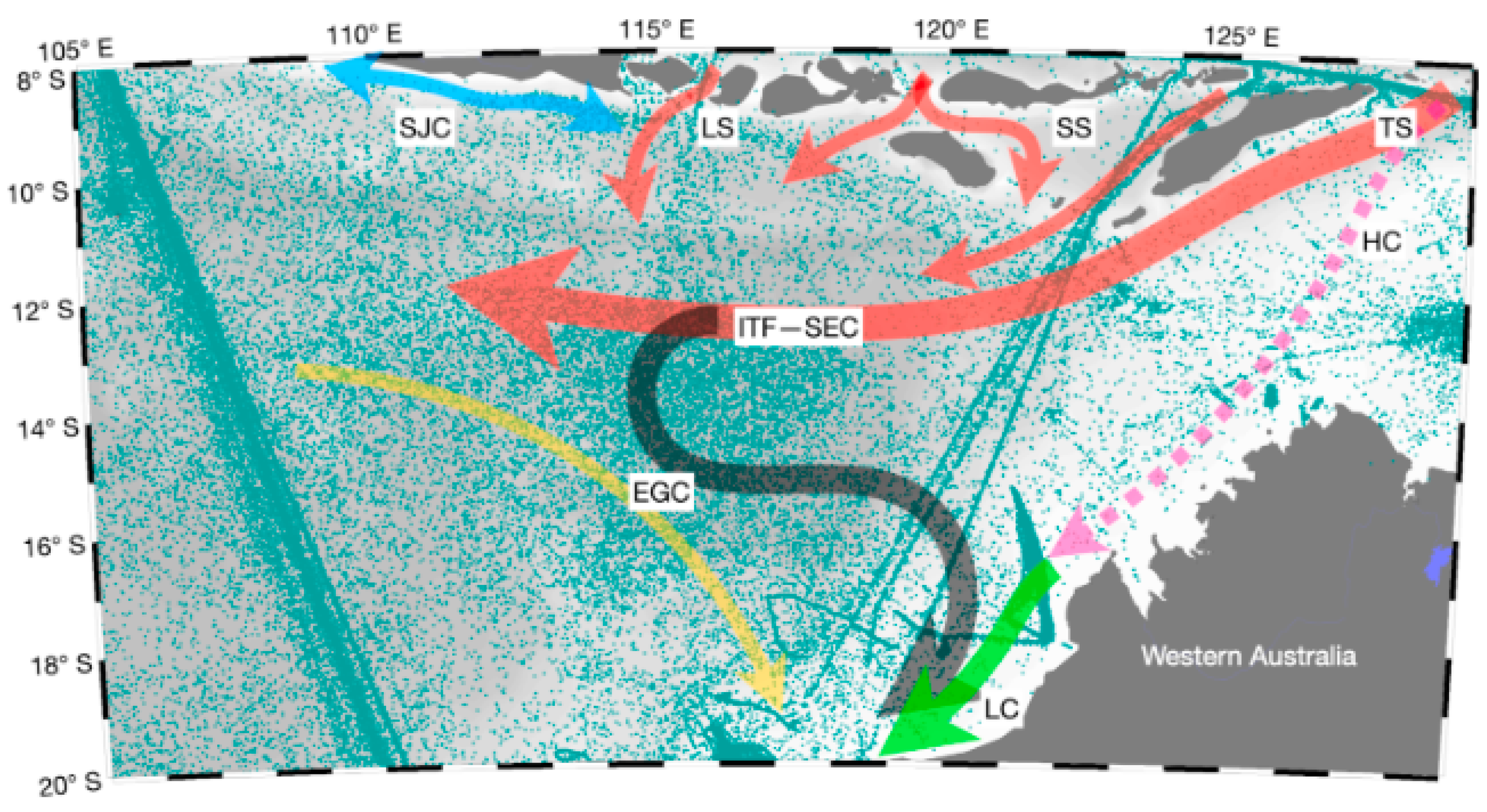
2.1. Geographical Areas
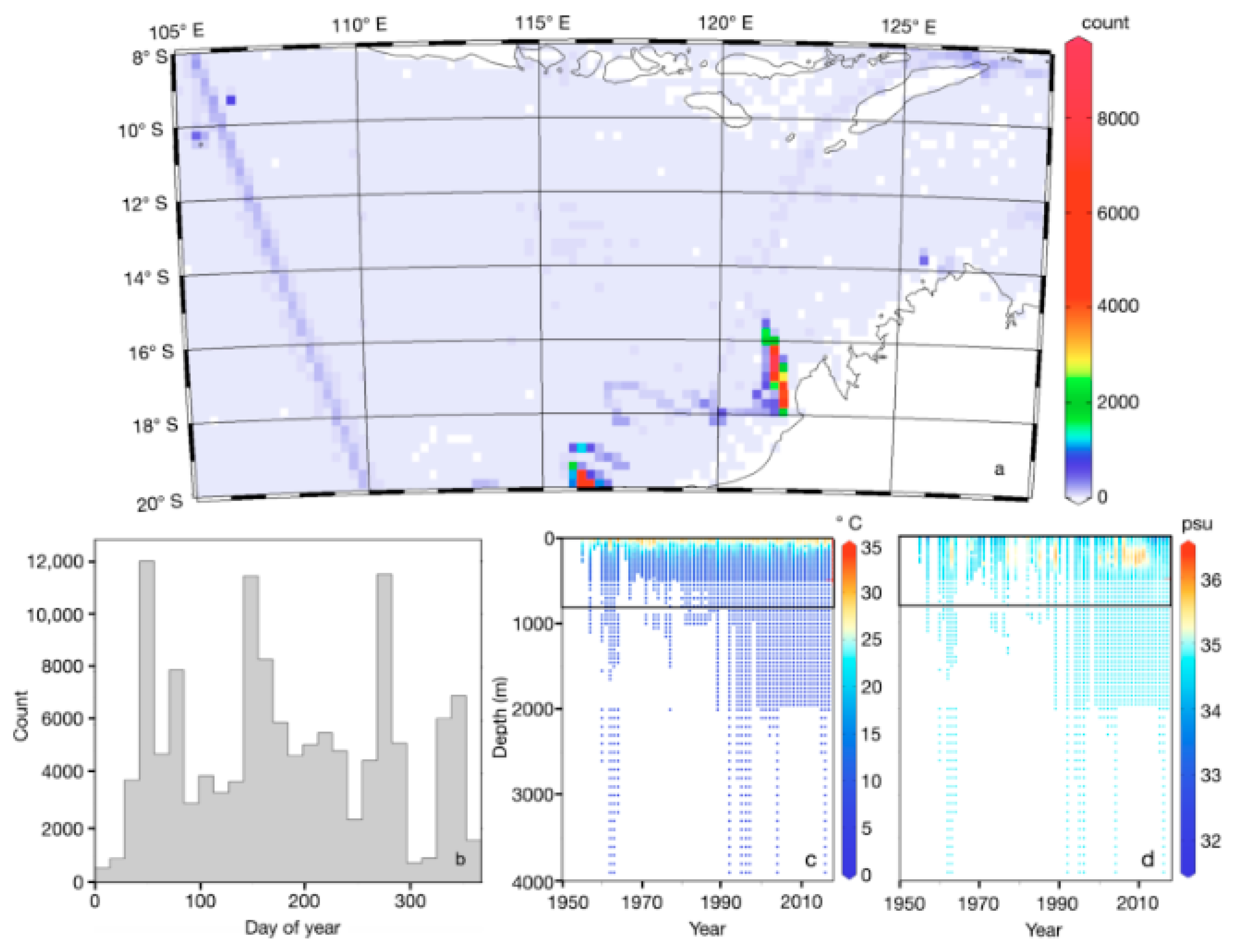
The area of interest for this study extends from 8° S to 20° S and 105° E to 129° E (Figure 1). This area has a complex circulation due to its interaction between the North and South Pacific Ocean, the Central Indian Ocean, and the Indonesia Seas. The ITF flows from the Pacific to the Indian Ocean through the Indonesia Seas (IS), mostly in the eastern sides. In the outflow, the ITF characteristics can be seen around 10° S to 20° S near the north of Australia. Several straits passed by the ITF include the Savu, Ombai, and Lombok Straits [7]. The annual average surface transport for the ITF is around 5–7 Sv (Sv ≡ 106 m3 s−1) [7], while the LC transport near West Australia is about 2.5 Sv [26]. Furthermore, both the ITF and Holloway Currents (HCs) are branches of surface currents originating from the Banda Sea through the Timor Sea.
As a result of the difference in sea surface elevation in the EIO waters, the surface currents flow from several straits in the southern part of the Indonesian archipelago, such as the Lombok Strait, with a speed of 2.6 Sv. Subsequently, from the Sumba Strait, it flows into the Indian Ocean through two branches, where one stream directly enters the Indian Ocean and the other flows through the Savu Strait. The ocean currents that flow in the eastern part originate from the Banda Sea and the Aru Sea, passing through the Ombai Strait in the western part of East Nusa Tenggara in the Timor Sea, with a velocity of 4.9 Sv [29]. Previous studies have suggested that the current originating from the Timor Sea flows directly towards 12° S and then turns towards the subtropics (black arrow) due to the convergence of currents from the Western Indian Ocean. The velocity of the surface ocean currents exiting the South Banda Basin, which joins the Timor Passage, is approximately 7.5 Sv [29]. However, other research indicates the existence of pathways that flow towards Western Australia, known as the Holloway Currents (HCs) [14]. In addition, in the south of Java, there is a current that flows annually called the South Java Currents (SJCs) [30]. This current strengthens during the Asian monsoon and experiences a decrease in speed during the Australian monsoon due to its interaction with the ITF in the Lombok Strait.

2.2. Datasets

The data used for analysis were the temperature and salinity, extracted from the World Ocean Database (WOD) 2018, which covered the study area. Both parameters were derived from the field measurement data. The data were first downloaded from the updated data for the global archive (https://www.ncei.noaa.gov/access/world-ocean-database-select/bin/dbsearch.pl) (accessed on 17 June 2023). The WOD was chosen as the data source, since it provides a wide range of in situ measurements, including physical, chemical, and biological oceanography [31]. Further, the accuracy level of the data generated by instruments in the WOD is very high, e.g., 0.2 °C for XBT [32]. The available datasets were mainly from the XBT instrument, with a total data casting of 252,136 data points from 1950 to 2018 (Table 1). The vertical data used were the standard level/depth, which means a depth below the sea surface at which water properties should be measured and reported. The data were then collected and analyzed from the surface to a depth of 800 m, based on the availability of data from the WOD 18 in the Eastern Indian Ocean (EIO). However, this depth already represented three different layers, i.e., mixed, thermocline, and deep layers.
The geographical distribution of the dataset revealed that the temperature and salinity data were distributed across all areas, with the number of datasets below 1000. However, in certain regions, particularly those adjacent to Western Australia, there was an abundance of datasets exceeding 1000, primarily sourced from glider data. Additionally, when observing the daily data distribution, it was evident that, from the first quarter to the third quarter, there were data points exceeding 10,000, except for the fourth quarter (Figure 2).
The highest temperature in the upper layer of the study region was recorded in August 1994 (32.4 °C), while the lowest temperature in the deep water was recorded in 2015 (1.2 °C). This condition coincided with the highest salinity in the upper layer recorded in August 1994 (36.1 psu), and the lowest salinity in the deep water recorded in 2008 (30.6 psu) (Table 2).
Temperature and salinity data were visualized on a monthly basis, which was separated into two main monsoons. The northwest monsoon (NWM) represents the data from December to February (DJF), and the southeast monsoon (SEM) represents the data from June to August (JJA).

2.3. Data Analysis

Before being analyzed, the raw data were filtered into good-quality data/flags. For this area, the outliers for temperature and salinity, which are outside −3 to 35 °C and 20 to 40 psu, respectively, were removed [33]. The weighted-average gridding interpolation method was used in scalar values, and XBT/MBT corrections were done according to NCEI Guidance and correction schemes (http://www.nodc.noaa.gov/OC5/XBT_BIAS/xbt_bias.html) (accessed on 9 October 2023) [34,35].
To identify the water mass, the T-S time (seasonal T-S) diagram plots were employed. The T-S time was provided by salinity and potential temperature using TEOS-10. In a T-S diagram, the potential temperature (on the vertical axis) is plotted versus the salinity (on the horizontal axis) and combined with the density for two seasons. The density values were calculated from each dataset using the equation of the state of the seawater. The T-S time diagram was employed to depict the simultaneous relationship between the temperature and salinity across different vertical depths and different seasons of the seawater column. Furthermore, water mass types were widely used to analyze the structure of the stratification and mixing in the water column [36]. In this study, the concepts and definitions were classified and defined the key properties of main water masses in the EIO based on WOD-18 data products by referring to previous findings (Table 3) [6,36].
Furthermore, the stability of the water column was analyzed based on the variable derivation of the Brunt-Väisälä Frequency (BVF), which can be calculated by the Equation [37,38,39]:
N = g ρ 0 p ( z ) ( z ) ,
where N represents a vertically displaced water parcel that oscillates (cycle/h); g is the acceleration due to gravity (9.8 m·s−2); ρ 0 is the average density of the measurement results (kg·m−3); z is the depth (positive upward). The N2 was acquired from the absolute salinity and conservative temperature values [40]. For N, a value greater than 0 indicates a stable layer, and a value smaller than 0 indicates an unstable layer. For additional analysis, three section transects were made at 8° S, 12° S, and 16° S to observe the dynamics of the temperature and salinity.

3. Results

3.1. Seasonal T-S Variation

There are distinct variations in temperature and salinity between the surface and the layers of water below in both seasonal conditions. In general, the surface temperature is elevated, accompanied by lower salinity levels, which contributes to the warmer conditions compared to the lower layer in both seasons. Furthermore, the warmer areas were observed at lower latitudes for both the surface of the waters and deep layers, with warmer areas in the deeper layers specifically situated in subtropical areas (Figure 3).
During the NWM season (Figure 3a), data showed a gradual decrease in temperature on the surface layer. The average temperature on the surface was warmer (27.5 °C) compared to the deep layer (10 °C; Figure 3e). On the surface, temperatures ranged from 25.0 to 27.5 °C, whereas cooler water temperatures were found in subtropical areas (16 to 20° S; Figure 3a). In some regions, such as the Bali Strait, southern Bali, the eastern part of southern Java, and the southern Savu Sea, warmer temperatures of approximately 28.5 °C were observed in comparison to the surrounding areas (Figure 3a). At the surface, higher salinity values (ranging between 34.5 and 35.0 psu) were located between 16 and 20° S (Figure 3a). Lower salinity levels, approximately 33.5 psu, were observed in various locations close to the Indonesian islands, including the southern Java, southern Bali and surrounding areas, as well as the Savu Sea (Figure 3a). At the mixed layer (Figure 3c), temperatures ranged between 15 and 21 °C. Regions with a temperature of 15 °C were recorded around the south of Java (9° S), and the warmest was in Northwest Australia and the far side of Southern Indonesia (18° S; Figure 3c). Closer to the subtropic area, the temperature became warmer (19 to 20 °C) compared to Java Island (15 to 19 °C; Figure 3c). At this particular depth, the salinity distribution in the waters near the Indonesian islands appeared to be quite uniform, with salinity values ranging between 34.0 and 34.5 psu. However, moving further south beyond the latitude of 16° S, a distinct change in the salinity pattern was evident (Figure 3c). The salinity values in this region ranged from 35 to 36 psu, showcasing a slightly higher concentration of salts compared to the waters near the Indonesian islands. Moreover, this increase in salinity appeared to be evenly distributed from the west to east regions.
At the deep layer (Figure 3e), temperatures were generally more homogeneous from the east to the west, with values ranging from 7.5 to 8.0 °C. The temperature difference between waters close to Indonesia and more distant waters was approximately 1 °C (Figure 3e). Colder regions were recorded in the Savu Sea, Lombok Strait, and its surroundings, with temperatures of around 7 °C. The highest temperature value at this depth was approximately 8 °C, located at the south of Java (Figure 3e). Within the latitudes from 12 to 16° S, the temperature remained relatively homogenous, ranging between 7.2 and 7.4 °C. Regarding the salinity conditions, the water with higher salinity values were primarily located in the subtropical regions (except for the deeper depths), where a higher salinity of 34.7 psu was observed at the south of Java Island, while lower salinity was recorded in the Savu Sea and the far side of western Australia (20° S; Figure 3e). In the central regions, the salinity hovered around 34.6 psu.
During the SEM (Figure 3b), the sea surface temperature ranged between 24.0 and 27.5 °C. The western part of the Indonesian archipelago was warmer (27.5 °C) compared to the eastern part (26 °C; Figure 3b). The temperature between latitudes of 12 and 16° S was almost homogeneous, with a value of 27.5 °C. Approaching the subtropical latitudes, the temperature became cooler again, ranging within 24.5–25 °C. There were no significant temperature differences observed between the western and eastern regions at this depth (Figure 3b). In contrast to the temperature, the salinity values highlighted significant variations, especially in regions close to Indonesia (Figure 3b). The southern waters of Java demonstrated elevated salinity levels of 34.5 psu, whereas the eastern waters of Indonesia displayed comparatively lower salinity values ranging between 33 and 34 psu (Figure 3b). Similar salinity patterns were also observed from the 12 to 16° S latitudes. Moving to higher latitudes, the salinity demonstrated an increasing trend, spanning from 34.5 to 36 psu, with the maximum salinity value recorded on the far side of Australia (Figure 3b).
In the mixed layer (Figure 3d), the sea surface temperature near Indonesian waters were observed to have a homogeneous level, ranging between 15.0 and 17.5 °C. Elevated temperature values were found around the Savu Sea, while lower values were located at the south of Java. As the region approached the 14° S latitude, the temperature elevated to 19–20 °C, and these values continued dominantly across the area from the western to the eastern waters adjacent to Australia (Figure 3d). Within the latitudes ranging from 14 to 20° S, higher temperature values were observed along the coast of Australia compared to the area in the western waters. In terms of the salinity, the values were homogeneous from the west to the east Indonesian waters, persisting at ~34.5 psu (Figure 3d). The salinity value remained relatively constant until the 14° S latitude. Beyond those points, the salinity levels increased to the range 35–36 psu, with the exception of coastal Australia, where the salinity remained approximately 34.5 psu (Figure 3d).
At the deep layer (Figure 3f), the sea surface temperatures exhibited a range between 7.2 and 8.0 °C. Moreover, the highest temperature values were observed in the waters situated to the south of Java, in contrast to the cooler temperatures present around the Savu Sea and the far side of Australia. The waters to the south of Bali had a temperature of approximately 7.4 °C. Within the latitudes from 12 to 16° S, the water temperatures ranged between 7.4 and 7.6 °C. Moving further south to latitudes of 18 to 20° S, the temperatures ranged from 7.2 to 7.8 °C, with the highest value found near the coast of Australia. Concurrently, the salinity values near Indonesian waters varied between the western and eastern parts (Figure 3f). In the western part (south of Java), the salinity was higher (34.7–34.8 psu) in comparison to the eastern part, with a maintained salinity value of 34.5 psu (Figure 3f). Within the latitudes from 12 to 16° S, the salinity was measured at approximately 34.6 psu and remained a consistent trend from east to west. In the higher latitudes (18 to 20° S), higher salinity values of 34.6 psu were evident in the eastern part, close to the waters of Australia, while the western part had a salinity of ~34.5 psu (Figure 3f).
Across different latitudinal sections during both the NWM and SEM, distinct temperature and salinity patterns within the water columns emerged. Vertically, the temperature and salinity profiles varied significantly along each transect. Generally, in both seasons, warmer temperatures were found at the surface and gradually decreased with depth. In contrast, below the thermocline, the temperature decreased slowly with increasing depth. Salinity profiles were more complex than the temperature profiles, where the values generally increased with the increasing depth (Figure 4).
During the NWM season, the surface temperature ranged from 25.0 to 28.5 °C at 8° S (Figure 4a). Regions characterized by lower temperatures were identified in the Lombok Strait, while warmer waters were observed in the Timor Sea (~27.8 °C; Figure 4a). Moving downward, the temperature values became colder, and the thermocline layer during the NWM started at a depth of 50 m (Figure 4a). In the deeper layer, the temperature became slightly homogenous, with values below 10 °C (Figure 4a). Furthermore, the surface salinity varied between 34.0 and 34.5 psu (Figure 4a). Lower salinity values were recorded around the longitude of 115° E, particularly near the Lombok Strait. As we moved downward, the salinity increased and exceeded 34.5 psu (Figure 4a). Within water depths between 400 and 800 m, the western part (105 to 112° E) exhibited a slightly higher salinity (34.7 psu) compared to the eastern part near Australia (34.5 psu).
At 12° S (Figure 4c), the surface temperature showed a warmer trend within the waters of the Savu Sea (30 °C) in contrast to its surrounding areas (Figure 4c). Moving to the deeper layers, the temperature gradually decreased to 17.5 °C at a depth of 200 m (Figure 4c). In the deep layer, the temperature started at 12.5 °C and continued to decline with increasing depth, reaching minimum at the 800 m depth (Figure 4c). Meanwhile, the surface salinity varied between the eastern and western parts. In the eastern part, low salinity values (34 psu) were observed around 122.5° E, which was close to the coast of Australia (Figure 4c). As depths increased to the range from 200 to 800 m, there was a salinity difference between the eastern and western parts (Figure 4c). The western part (105 to 115° E) had a salinity value of 34.7 psu, while the eastern part (near Australia) had a salinity value of 34.5 psu.
At 16° S (Figure 4e), the temperature ranged from 25.0 to 28.0 °C in the mixed layer, with warmer values located around 110° E. Moving to the deeper layers, the temperature decreased from 25.0 to 10.0 °C at a depth of 400 m (Figure 4e). In the deeper layers, the temperature appeared to be more uniform compared to the upper layers. There were no significant temperature differences documented between the eastern and western waters (Figure 4e). Regarding the salinity within the mixed layer, there was a minimal variation observed between the western and eastern parts. The surface salinity values ranged from 34 to 35 psu (Figure 4e). Lower salinity values were recorded within the regions between 105 and 110° E, and 115° E and 120.0 to 122.5° E. At depths ranging from 150 to 400 m, the salinity levels were higher in the western part (between 105.0 and 117.5° E; Figure 4e), with values ranging between 34.7 and 35.5 psu (Figure 4e). Meanwhile, in the western part, near the coast of Australia, the salinity remained consistent around 34.5 psu. In the deep layer (after 400 m), the salinity became more uniform, maintaining a value of approximately 34.7 psu.
During the SEM, the surface temperature at 8° S (Figure 4b) demonstrated a range from 25.0 to 27.5 °C. Regions with lower temperatures were found in the Savu Sea, while warmer regions were observed in the waters south of Java. Within the region of the Savu Sea region, the mixed layer’s depth was highlighted as deeper compared to its surrounding areas, reaching a maximum depth of approximately 150 m (Figure 4b). At depths below the mixed layer, the temperature profile reached 15.0 °C at a depth of 200 m. In the deep layers, the temperature demonstrated a higher homogeneity, with values below 10.0 °C. Regarding the salinity, the surface values ranged from 34 to 34.5 psu, where lower salinity values were found in the region around the Savu Sea (122.5° E; Figure 4b). At depths ranging from 200 to 800 m, there were significant differences in the salinity of the water column between the western and eastern parts. Between 105 and 115° E, the salinity reached its maximum peak value at 34.7 psu, whereas, in the eastern part, the salinity remained around 34.5 psu (Figure 4b).
At 12° S (Figure 4d), the temperature within the mixed layer demonstrated a range from 25.0 to 28.0 °C, with warmer values located around 105° E. Moving to the deeper layers, the temperature gradually decreased from 25.0 °C to 10.0 °C at a depth of 400 m. In the deeper layers (>400 m), the temperature appeared to be more uniform compared to the layers above, and there were no significant temperature differences between the eastern and western waters (Figure 4d). For the salinity profiles in the surface layers, the values ranged from 34 to 34.5 psu. Higher salinity values were observed near the coast of Australia (Figure 4d). At depths ranging from 150 to 800 m, the salinity reached its maximum between 105 and 117.5° E, with values ranging from 34.7 to 35.5 psu, and the highest value occurred at a depth of 400 m (Figure 4d). In the western part, near the coast of Australia, the salinity remained around 34.7 psu.
In the mixed layer at 16° S (Figure 4f), temperature variations were significantly observed between the western and eastern parts, with values ranging from 26.0 to 27.0 °C (Figure 4f). Warmer temperatures were observed around 110 to 120° E (Figure 4f). Moving to the deeper layers, the temperature decreased to 10.0 °C at a depth of 400 m. In the deeper layers, the temperature became more uniform compared to the layers above, and there were no significant temperature differences between the eastern and western waters (Figure 4f). Regarding the salinity profiles in the mixed layer, there were significant variation levels between the western and eastern parts. Surface salinity values ranged from 34 to 34.7 psu (Figure 4f). Lower salinity values were found between 105° E and 110° E. Specifically, around 115° E, the highest salinity value of 34.7 psu was observed. Within 100 to 400 m, the highest salinity values were identified between 105° E and 117° E, ranging from 34.7 to 35.5 psu, with lower salinity in the western part near the coast of Australia (Figure 4f). In the deep layer (below 400 m), the salinity became more uniform, with a value of ~34.5 psu.

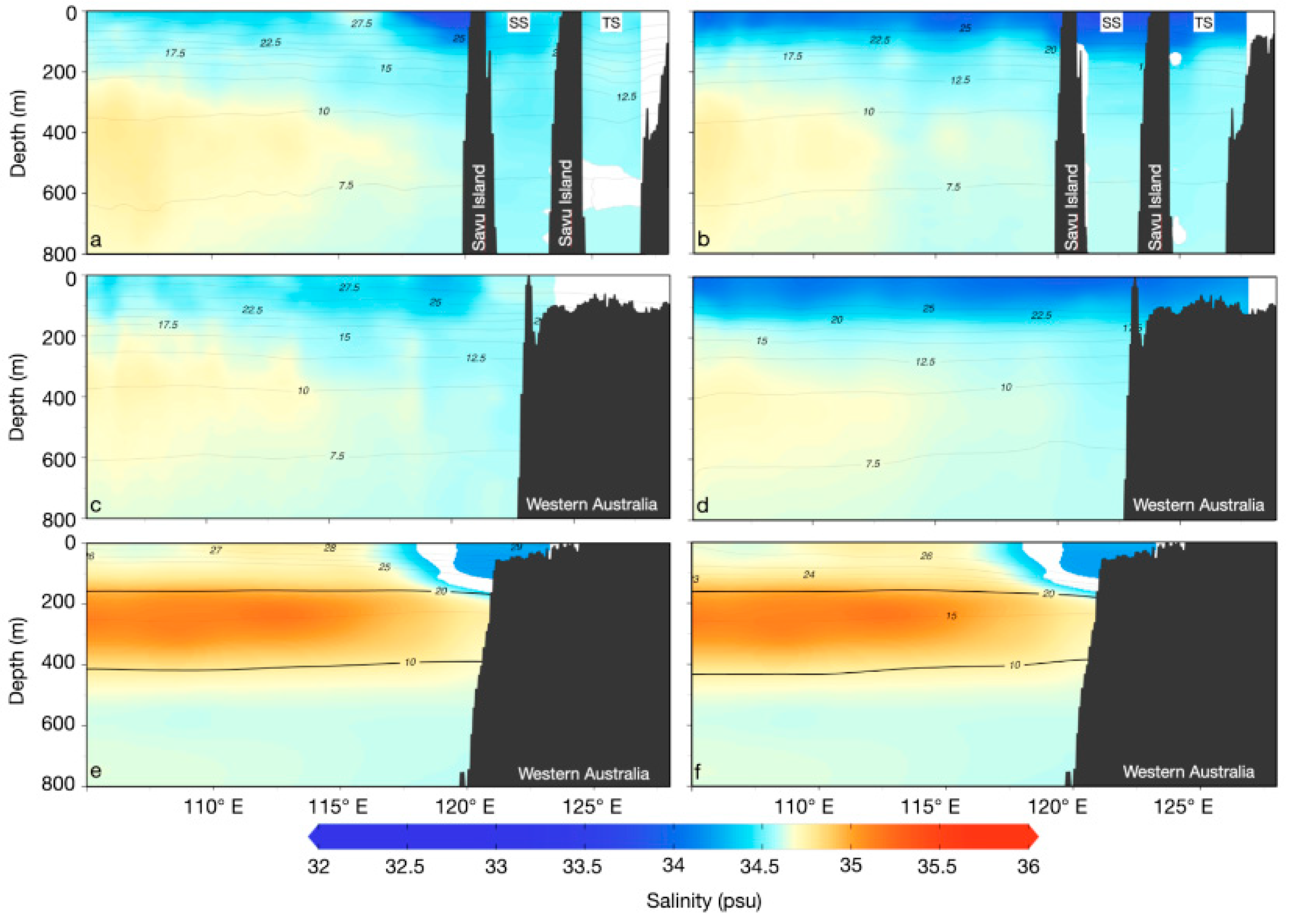
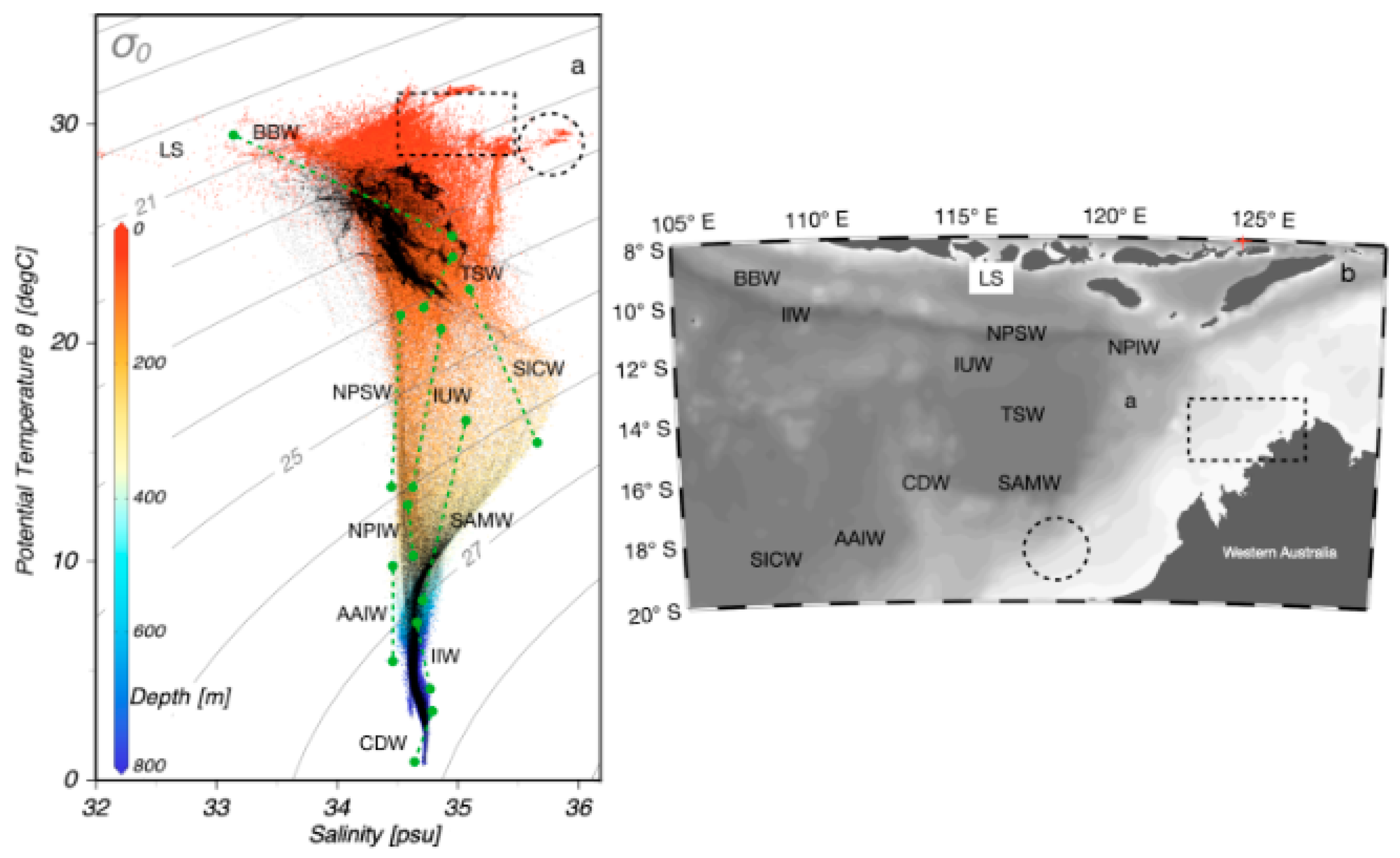
3.2. Water Mass Structures

In general, there were no significant differences in the types of water masses found between the two monsoon seasons, except for the Arabian Sea Water (ASW), which was not found during the northwest monsoon. Our result showed there were ten types of water mass classes distinguished in the study area. The upper layer of the water column was dominated by IUW, BBW, SICW, and TSW In the following layer, there were SAMW, NPIW, NPSW, AAIW, and IIW. In the bottom layer, there was CDW (Figure 5).
The salinity range observed during the NWM highlighted a wider span in comparison to the SEM (Figure 5), a distinction particularly observed at a depth of 200–250 m (Figure 5). In the surface layer, it was characterized with warm (25 to 32 °C) and low-salinity (32 to 35 psu) water. Water masses, such as Bengal Bay Water (BBW) and Arabian Sea Water (ASW), were found in the south of Java. The IUW water mass was found between 200 and 400 m, which was dominated by the water from Indonesia. This water mass was still visible up to a 150 m water depth. In the northern regions, various areas were identified as hosting North Pacific Intermediate Water (NPIW), including the strategically positioned Lombok Strait (115° E) and Ombai Strait (125° E). The NPSW is characterized by its subtropical origin, featuring warm temperatures, relatively low nutrient concentrations, and lower salinity compared to surrounding waters. In both monsoons, the TSW water mass was found at a depth of 150 m with a salinity value of around 35 psu. The SICW water mass was more saline compared to other water masses. The SICW had a salinity maximum of 35.1–35.9 psu and was located between 200 and 400 m, extending from 105 to 110° E. The IIW water mass was found at a depth of 600 m with a salinity value of around 34.6 psu and a temperature of 8.6 °C. Furthermore, the water masses in the deep layer also included the SAMW, which was recorded at a depth of 700 m. At the bottom layer (800 m), distinctive water masses were identified, such as the AAIW and CDW. The AAIW was identified at 16° S within the latitudes between 105 and 110° E.

3.3. Water Column Stability

The water column stability throughout the NWM and SEM across the three transects demonstrated significant variations from the surface down to the deep layers (Figure 6). In general, the unstable layer was found at the surface and deep layers (Figure 6). Furthermore, the stable layer was located at water depth ranging between 50 and 150 m, with BVF values of around 8 to 13 cycles/h (Figure 6).
During the NWM, at latitude 8° S (Figure 6a), in the surface, the BVF range was observed in the range from 3 cycles/h to 10 cycles/h. More stable areas were in the waters of the Savu Sea (120° E) and Timor Sea (125° E), while less-stable areas were observed south of Java (105° E), south of Bali (112° E), and the Lombok Strait (115° E). Furthermore, at a depth of 50 m to 250 m, the water column became more stable, with a value of 10 cycles/h. Between depths of 400 m and 800 m, the BVF value ranged from approximately two cycles/h to three cycles/h. At latitude 12° S (Figure 6c), the surface showed an unstable layer up to 30 m, with values ranging from two cycles/h to five cycles/h. A more stable layer was observed at a depth of about 50 m, with a value of ~10 cycles/h. At a depth of 200 m, the value was ~five cycles/h, and continued to decrease to a depth of 800 m, with a BVF value of two cycles/h. At latitude 16° S (Figure 6e), at the surface water, the BVF values ranged from two cycles/h to five cycles/h. As the depths increased from 30 m to 250 m, the water column became more stable, with a value of ~10 cycles/h. At the next depth (250 m to 800 m), the values were from two cycles/h to five cycles/h, with the unstable layer being in the deep layer.
During the SEM, at latitude 8° S (Figure 6b), in the surface, the BVF value was in the range from 3 cycles/h to 10 cycles/h. The more stable areas were in the waters of the Savu Sea and Lombok Strait, while the more unstable ones were south of Java, south of Bali, and the Timor Sea. Furthermore, at a depth from 50 m to 250 m, the water column became more stable, with a value of 10 cycles/h. From a depth of 400 m to 800 m, the value was about two cycles/h to three cycles/h. At latitude 12° S (Figure 6d), in the surface, characterized by an unstable layer up to 70 m, the BVF ranged from one cycle/h to five cycles/h. There was no significant difference from the eastern to the western areas. The more stable layer was at a depth of about 70 m, with a value of ~10 cycles/h. At a depth of 200 m, the BVF value was ~five cycles/h and continued to decrease to a depth of 800 m, with a value of two cycles/h. At latitude 16° S (Figure 6f), at the water level (up to 50 m), the BVF values ranged from one cycle/h to five cycles/h. Furthermore, at depths of 50 m to 250 m, the water column became more stable, with a value of ~10 cycles/h. At the next depth (250 m to 800 m), the BVF value was two cycles/h to five cycles/h, with the unstable layer being in the deep layer.

4. Discussion

The analysis of the temperature and salinity data from the WOD highlighted a general structure of the EIO characteristics. In general, warmer and low-salinity water existed in the lower latitude and surface waters. Due to regions mostly located in the tropical regions, the heat from the atmosphere influenced the surface layer directly. Along with that, a colder temperature and higher salinity existed in the subtropical area (Figure 3 and Figure 4). On the surface, some of the regions (Figure 3a) were characterized by lower salinity (~34 psu) and warmer temperatures (>24 °C), which were found near the ITF outflow. Water masses with lower salinity (34.5 psu) were clearly visible in the Lombok Strait during the NWM. Conversely, these low-salinity water masses were found in the Lombok Strait and Savu Sea during the SEM. This lower salinity present during both seasons (Figure 3a,b) suggested the presence of freshwater input originating from the Indonesian Seas [7]. However, the intensity of the SJV through the coastal Java Seas influenced the spreading of water masses to the Indian Ocean, especially from the Lombok Strait [30]. The new water mass formed during the transit through the Indonesian archipelago from the Pacific Ocean [41]. It was reported that the ITF had the strongest velocity in the SEM and influenced the spreading of the water mass. The water mass characteristics can reach up to 14° S near the Great Barrier Reef (GBR) of Northern Australia. The ITF transport in the SEM is faster compared to the NWM and confirms previous observations [7,33]. Furthermore, the river inputs from the islands in the Java Seas, Banda Seas, and its surroundings, as well as the presence of intense precipitation, influenced the mixing process in the Indonesian waters [33] and the interaction between the upper ocean and lower atmosphere [42,43]. During the NWM season, the thermocline started at a depth of 50 m, indicating a strong stratification in the upper layers of the ocean. This stratification was influenced by the seasonal wind patterns and vertical mixing processes [7]. During the SEM, winds originated from the Australian continent blew towards Asia, generating surface currents in the EIO to the Central Indian Ocean, and near Indonesian regions (Figure 3b). Our results showed a clear difference in the characteristics of the salinity and temperature between South Java and the straits in the eastern part. This phenomenon occurred due to the convergence between the SJV and ITF flowing through those straits [44].
Regarding the LC, previous observations had mentioned a correlation between this current system and the ITF. In this study, the LCs were observed at 16° S in shallow (<200 m) water, with a narrow band (~100 km wide) of warm (~29 °C) and lower-salinity (<34 psu) water (Figure 4d,e). The LC waters transferred water mass to the subpolar region via Western Australia. Furthermore, the LC was characterized by the water mass from the ITF and Central Indian Ocean [20], where it transported warm and low-salinity water. Moreover, both the LC and ITF demonstrated a strong seasonal pattern during the Australian winter (SEM) [45]. However, the current dataset may have limitations in providing detailed information about the dynamics between the Indonesian Throughflow, Holloway Currents, and Leeuwin Currents.
In between 8 and 14° S latitude (Figure 3c,d), the temperature and salinity values were more uniform along the 150 m transect. In this water column, the temperature was cooler in both seasons, with a range from 15 to 19 °C and a salinity value of 34.5 psu. This salinity characteristic was also evident in a previous study by [44]. Meanwhile, at latitudes from 16 to 20° S, the water mass was warmer (20 to 21 °C), with a salinity value of 34.9 psu that tended to decrease towards the east (Western Australia) due to input from the Central Indian Ocean. Additionally, at 600 m in the northern region, warmer water temperatures (7.8 to 8 °C) were found in south Java. In comparison, lower temperatures were found in the east (Savu Sea and its surroundings), with values extending between 7.0 and 7.2 °C. The presence of the warmer water in the west is believed to be caused by the input from the Indonesian Seas and shallow water in Western Australia.
At latitudes ranging from 12 to 18° S, the temperature and salinity values tended to be more homogenous. Specifically, at the 20° S latitude, the temperature and salinity values were lower in the west (~7.4 °C and 34.5 psu) due to input from the CDW. In the deepest waters, the temperature elevated toward the bottom entirely due to the high pressure that compressed the water and raised its temperature adiabatically (Figure 4).
The surface layer, also called the mixed layer, exists at the surface and is mainly mixed due to external forces, such as wind stress and tides [33]. The types of water masses in this region represent the branch of the global thermohaline circulation, as displayed in Figure 5. In the upper and deep layers near the Lombok Strait, the water mass profiles and characteristics signaled a signature of the ITF, with a salinity of about 34.5–34.7 psu [43]. The mixed layer in the NWM was shallower compared to the SEM (Figure 4) due to the wind blowing from Australia from June to August, forcing the surface water mass to move towards the Central Indian Ocean [2] (Figure 7).
The warm and low-salinity water was observed around the 200–300 m depth, which corresponded to the high-salinity core of the TSW. This type of water mass is typically formed in the winter season (around 30° S), reflecting the evaporation process, and was carried to the northern regions by the large-scale interior anticyclonic circulation. Below the SICW, a water mass identified as the SAMW occurred at 350–600 m (Figure 5). The AMW showed a minimum salinity (34.4 to 34.6 psu), indicating the presence of the AAIW along the western coast of Australia [46]. Furthermore, in line with the result from [47], this water mass was also observed near the coast of Australia (120° E; 16° S), which flows from the Antarctic. The SAMW is formed by deep winter convection at 40–50° S in the zone between the subtropical convergence and the subantarctic front to the south of Australia [48]. Below the SAMW and SICW, the presence of the AAIW with a salinity minimum (34.4–34.6 psu) was observed. Furthermore, the AAIW extends northward from the Antarctic polar front to latitudes of 10–15° S [47]. However, in the deep layer, the AAIW exists near 16° S. The AAIW is the main intermediate water in the South Atlantic Ocean, and this water mass formed in the Antarctic polar zone [49]. Moreover, the AAIW is modified by mixing with the IIW, which is carried to the CIO [48]
Furthermore, the stability of the surface water column during the SEM was deeper than the NWM (Figure 6). At 8° S (NWM), the thickness of the mixed layer is caused by the winds blowing from Australia towards Asia through Indonesia. Typically, these winds blow from June to August each year. The interaction between the winds and the surface waters causes the mixed layer to become thicker. Ocean currents from Western Indonesia, specifically the SJC, predominantly contribute to the significant gradient between the surface and the thermocline in the western part [50]. At latitudes between 12 and 16° S (SEM), the differences in thickness were due to surface equatorial currents that flow toward the Central Indian Ocean. This leads to an additional layer of thickness up to 50 m compared to the NWM. At latitude 16° S, the decrease in water heating and the inflow of water from Antarctica caused the middle to lower layers to have homogeneous temperatures and salinity levels. Therefore, there was no significant difference between the depths of 50 and 800 m, suggesting the stability value was almost similar, which is a different observation compared to transects of 8 and 12° S in the whole water column.

5. Future Challenges

The World Ocean Database provides much information about water mass dynamics and stability from 0 to 800 m in the EIO. However, based on Figure 2c and Figure 3a, the available data (1950–2018) are insufficient to analyze the dynamics of water masses, especially from 800 m to the deeper layers. Additionally, the current dataset may have limitations in providing detailed information about the dynamics between the ITF, HC, and LC. Therefore, to enhance our understanding of these complex circulations, future research should consider observing coastal areas, including Northwestern Australia and the Timor Sea regions.
In the era of global warming, long-term observational data are required to enhance our understanding of the complexities and variations in water mass behavior within this depth range. The deep-water layers are increasingly being impacted by global warming, experiencing changes in temperature and circulation patterns [51]. Previous findings have stated that various regions (the Atlantic, Pacific, and Arctic Oceans), particularly in deep water, have already been influenced by global warming [52,53,54]. The Eastern Indian Ocean (EIO) is recognized for its rich biodiversity, notably featuring coral reefs and marine megafauna. Several publications have stated that ocean temperature and salinity changes have influenced the ecosystem in the context of climate change, emphasizing the need for continued research to mitigate the impacts on marine life and global climate systems [55].

6. Conclusions

In situ data (68 years) from the WOD 18 have shown water column dynamics in the EIO areas. The study of temperature, salinity, and water column stability was undertaken to understand the water mass characteristics in this region. Using the temperature and salinity parameters as a proxy, the unique characteristics between water column layers have been clearly revealed. The warmer and less-saline waters were located near Indonesia and correlated with the inputs from the Indonesia Seas. Moving towards the subtropical regions, the temperature tended to decrease, while the salinity was likely to increase. Furthermore, the T–S seasonal diagram was the best approach to portray the type of water masses over the transects in this study. The water mass in the Eastern Indian Ocean (EIO) comes from several sources, including the Pacific, Indian, and Arctic Oceans. Ten types of water masses exist in the EIO region, including IUW, BBW, ASW, TSW, SAMW, SICW, AAIW, IIW, and CDW, while the BVF value of the surface water for the SEM was thicker compared to the NWM.

Author Contributions

N.P.P.: conceptualization, writing—original draft preparation, and visualization. M.F.A.: supervision, writing—review and editing, and methodology. W.S.P.: formal analysis, writing—review and editing, and validation. S.: investigation and resources. Z.Z.: writing—review and editing, supervision, and validation. All authors have read and agreed to the published version of the manuscript.

Funding

This research was funded by Universitas Padjadjaran and the Institute of Oceanography and Environment (INOS), University Malaysia Terengganu.

Institutional Review Board Statement

Not applicable.

Informed Consent Statement

Not applicable.

Data Availability Statement

Data in this region are already enhanced and available on request. The raw data can be downloaded from the NOAA Atlantic Oceanographic and Meteorological Laboratory (AOML), and is publicly available through the NOAA National Centers for Environmental Information World Ocean Database (https://www.ncei.noaa.gov/access/world-ocean-database-select/bin/dbsearch.pl).

Acknowledgments

The authors thank N.H. for the important data information about the Indonesia Seas. We would like to express our gratitude to Y.K., B.P. and M.H.I. for their assistance in enhancing the quality of this paper. Additionally, we extend our appreciation to the INOS staffs, Komitmen Research Group (KGR) and Jack Don’t Swim (JDS) for their fruitful discussions.

Conflicts of Interest

The authors declare no conflict of interest.

References

  1. Kämpf, J.; Chapman, P. Upwelling Systems of the World: A Scientific Journey to the Most Productive Marine Ecosystems; Springer Science and Business Media LLC: Dordrecht, The Netherlands, 2016. [Google Scholar] [CrossRef]
  2. Utamy, R.M.; Purba, N.P.; Pranowo, W.S.; Suherman, H. The Pattern of South Equatorial Current and Primary Productivity in South Java Seas Rizky. In Proceedings of the 2015 5th International Conference on Environment Science and Biotechnology (ICESB 2015), Jinju, Republic of Korea, 9–10 November 2015; Volume 51, pp. 139–142. [Google Scholar] [CrossRef]
  3. Tussadiah, A.; Syamsuddin, M.L.; Pranowo, W.S.; Purba, N.P.; Riyantini, I. Eddy Vertical Structure in Southern Java Indian Ocean: Identification using Automated Eddies Detection. Int. J. Sci. Res. 2016, 5, 967–971. [Google Scholar]
  4. Sprintall, J.; Gordon, A.L.; Wijffels, S.E.; Feng, M.; Hu, S.; Koch-Larrouy, A.; Phillips, H.; Nugroho, D.; Napitu, A.; Pujiana, K.; et al. Detecting change in the Indonesian seas. Front. Mar. Sci. 2019, 6, 257. [Google Scholar] [CrossRef]
  5. Fan, W.; Jian, Z.; Chu, Z.; Dang, H.; Wang, Y.; Bassinot, F.; Han, X.; Bian, Y. Variability of the Indonesian Throughflow in the Makassar Strait over the Last 30 ka. Sci. Rep. 2018, 8, 5678. [Google Scholar] [CrossRef] [PubMed]
  6. Yuliardi, A.Y.; Atmadipoera, A.S.; Harsono, G.; Natih, N.M.N.; Ando, K. Analysis of characteristics and turbulent mixing of seawater mass in lombok strait. Ilmu Kelaut. 2021, 26, 95–109. [Google Scholar] [CrossRef]
  7. Atmadipoera, A.; Molcard, R.; Madec, G.; Wijffels, S.; Sprintall, J.; Koch-Larrouy, A.; Jaya, I.; Supangat, A. Characteristics and variability of the Indonesian throughflow water at the outflow straits. Deep. Sea Res. Part I Oceanogr. Res. Pap. 2009, 56, 1942–1954. [Google Scholar] [CrossRef]
  8. Song, Q.; Gordon, A.L.; Visbeck, M. Spreading of the Indonesian throughflow in the Indian Ocean. J. Phys. Oceanogr. 2004, 34, 772–792. [Google Scholar] [CrossRef]
  9. Sprintall, J.; Wijffels, S.E.; Molcard, R.; Jaya, I. Direct estimates of the Indonesian throughflow entering the Indian ocean: 2004–2006. J. Geophys. Res. Oceans 2009, 114, 2004–2006. [Google Scholar] [CrossRef]
  10. Sani, I.Y.; Atmadipoera, A.S.; Purwandana, A.; Syamsudin, F. Transformation and mixing of North Pacific Water Mass in Sangihe-Talaud in August 2019. In IOP Conference Series: Earth and Environmental Science; IOP Publishing Ltd.: Bristol, UK, 2021; Volume 944, p. 012053. [Google Scholar] [CrossRef]
  11. Feng, M.; Zhang, N.; Liu, Q.; Wijffels, S. The Indonesian throughflow, its variability and centennial change. Geosci. Lett. 2018, 5, 3. [Google Scholar] [CrossRef]
  12. Woo, M.; Pattiaratchi, C. Hydrography and water masses off the western Australian coast. Deep. Sea Res. Part I Oceanogr. Res. Pap. 2008, 55, 1090–1104. [Google Scholar] [CrossRef]
  13. Tillinger, D.; Gordon, A.L. Fifty years of the Indonesian throughflow. J. Clim. 2009, 22, 6342–6355. [Google Scholar] [CrossRef]
  14. D’Adamo, N.; Fandry, C.; Buchan, S.; Domingues, C. Northern sources of the Leeuwin Current and the ‘Holloway Current’ on the North West Shelf. J. R. Soc. West. Aust. 2009, 92, 53–66. [Google Scholar]
  15. Nof, D.; Pichevin, T.; Sprintall, J. ‘Teddies’ and the origin of the Leeuwin current. J. Phys. Oceanogr. 2002, 32, 2571–2588. [Google Scholar] [CrossRef]
  16. Wijffels, S.; Sprintall, J.; Fieux, M.; Bray, N. The JADE and WOCE I10/IR6 Throughflow sections in the southeast indian ocean. Part 1: Water mass distribution and variability. Deep. Sea Res. Part II Top. Stud. Oceanogr. 2002, 49, 1341–1362. [Google Scholar] [CrossRef]
  17. Auer, G.; De Vleeschouwer, D.; Smith, R.A.; Bogus, K.; Groeneveld, J.; Grunert, P.; Castañeda, I.S.; Petrick, B.; Christensen, B.; Fulthorpe, C.; et al. Timing and Pacing of Indonesian Throughflow Restriction and Its Connection to Late Pliocene Climate Shifts. Paleoceanogr. Paleoclimatol. 2019, 34, 635–657. [Google Scholar] [CrossRef]
  18. Feng, X.; Liu, H.L.; Wang, F.C.; Yu, Y.Q.; Yuan, D.L. Indonesian Throughflow in an eddy-resolving ocean model. Chin. Sci. Bull. 2013, 58, 4504–4514. [Google Scholar] [CrossRef]
  19. Silveira, T.M.; Carapuço, M.M.; Miranda, J.M. The Ever-Changing and Challenging Role of Ocean Observation: From Local Initiatives to an Oceanwide Collaborative Effort. Front. Mar. Sci. 2022, 8, 778452. [Google Scholar] [CrossRef]
  20. Makarim, S.; Sprintall, J.; Liu, Z.; Yu, W.; Santoso, A.; Yan, X.-H.; Susanto, R.D. Previously unidentified Indonesian Throughflow pathways and freshening in the Indian Ocean during recent decades. Sci. Rep. 2019, 9, 7364. [Google Scholar] [CrossRef]
  21. Levitus, S.; Antonov, J.I.; Baranova, O.K.; Boyer, T.P.; Coleman, C.L.; Garcia, H.E.; Grodsky, A.I.; Johnson, D.R.; Locarnini, R.A.; Mishonov, A.V.; et al. The world ocean database. Data Sci. J. 2013, 12, WDS229–WDS234. [Google Scholar] [CrossRef]
  22. Zweng, M.M.; Boyer, T.P.; Baranova, O.K.; Reagan, J.R.; Seidov, D.; Smolyar, I.V. An inventory of Arctic Ocean data in the World Ocean Database. Earth Syst. Sci. Data 2018, 10, 677–687. [Google Scholar] [CrossRef]
  23. Johari, A.; Akhir, M.F. Exploring Thermocline and Water Masses Variability in Southern South Cina Sea from The World Ocean Datbase (WOD). Acta Oceanol. Sin. 2019, 38, 38–47. [Google Scholar] [CrossRef]
  24. Chu, P.C.; Margolina, T.; Rodriguez, D.A.; Fan, C.; Ivanov, L.M. Spatial and temporal variability of the California Current identified from the synoptic monthly gridded World Ocean Database (WOD). Deep. Sea Res. Part II Top. Stud. Oceanogr. 2018, 151, 37–48. [Google Scholar] [CrossRef]
  25. Purwandana, A.; Cuypers, Y.; Bouruet-Aubertot, P.; Nagai, T.; Hibiya, T.; Atmadipoera, A.S. Spatial structure of turbulent mixing inferred from historical CTD datasets in the Indonesian seas. Prog. Oceanogr. 2020, 184, 102312. [Google Scholar] [CrossRef]
  26. Lambert, E.; Le Bars, D.; De Ruijter, W.P.M. The connection of the Indonesian Throughflow, South Indian Ocean Countercurrent and the Leeuwin Current. Ocean. Sci. 2016, 12, 771–780. [Google Scholar] [CrossRef]
  27. Tintoré, J.; Pinardi, N.; Álvarez-Fanjul, E.; Aguiar, E.; Álvarez-Berastegui, D.; Bajo, M.; Balbin, R.; Bozzano, R.; Nardelli, B.B.; Cardin, V.; et al. Challenges for Sustained Observing and Forecasting Systems in the Mediterranean Sea. Front. Mar. Sci. 2019, 6, 568. [Google Scholar] [CrossRef]
  28. Domingues, C.M.; Maltrud, M.E.; Wijffels, S.E.; Church, J.A.; Tomczak, M. Simulated Lagrangian pathways between the Leeuwin Current System and the upper-ocean circulation of the southeast Indian Ocean. Deep. Sea Res. Part II Top. Stud. Oceanogr. 2007, 54, 797–817. [Google Scholar] [CrossRef]
  29. Gordon, A.L. Oceanography of the Indonesian Seas and Their Throughflow. Oceanography 2005, 18, 14–27. [Google Scholar] [CrossRef]
  30. Utari, P.A.; Setiabudidaya, D.; Khakim, M.Y.N.; Iskandar, I. Dynamics of the South Java Coastal Current revealed by RAMA observing network. Terr. Atmos. Ocean. Sci. 2019, 30, 235–245. [Google Scholar] [CrossRef]
  31. Boyer, T.P.; Baranova, O.K.; Coleman, C.; Garcia, H.E.; Grodsky, A.; Locarnini, R.A.; Mishonov, A.V.; Paver, C.R.; Reagan, J.R.; Seidov, D.; et al. NOAA Atlas NESDIS 87. World Ocean Database 2018, 2018, 1–207. [Google Scholar]
  32. Parks, J.; Bringas, F.; Cowley, R.; Hanstein, C.; Krummel, L.; Sprintall, J.; Cheng, L.; Cirano, M.; Cruz, S.; Goes, M.; et al. XBT operational best practices for quality assurance. Front. Mar. Sci. 2022, 9, 991760. [Google Scholar] [CrossRef]
  33. Purba, N.P.; Pranowo, W.S.; Ndah, A.B.; Nanlohy, P. Seasonal variability of temperature, salinity, and surface currents at 0° latitude section of Indonesia seas. Reg. Stud. Mar. Sci. 2021, 44, 101772. [Google Scholar] [CrossRef]
  34. Cheng, L.; Zhu, J.; Cowley, R.; Boyer, T.; Wijffels, S. Time, probe type, and temperature variable bias corrections to historical expendable bathythermograph observations. J. Atmos. Ocean. Technol. 2014, 31, 1793–1825. [Google Scholar] [CrossRef]
  35. Cheng, L.; Luo, H.; Boyer, T.; Cowley, R.; Abraham, J.; Gouretski, V.; Reseghetti, F.; Zhu, J. How well can we correct systematic errors in historical XBT data? J. Atmos. Ocean. Technol. 2018, 35, 1103–1125. [Google Scholar] [CrossRef]
  36. Emery, W.J. Oceanographic Topics: Water Types and Water Masses. In Encyclopedia of Atmospheric Sciences, 2nd ed.; Elsevier: Amsterdam, The Netherlands, 2015; pp. 329–337. [Google Scholar] [CrossRef]
  37. Schlitzer, R. Ocean Data View. 2022. Available online: https://odv.awi.de (accessed on 17 June 2023).
  38. Emery, W.J.; Lee, W.G.; Magaard, L. Geographic and Seasonal Distributions of Brunt–Väisälä Frequency and Rossby Radii in the North Pacific and North Atlantic. J. Phys. Oceanogr. 1984, 14, 294–317. [Google Scholar] [CrossRef]
  39. Ferreres, E.; Soler, M.R.; Terradellas, E. Analysis of turbulent exchange and coherent structures in the stable atmospheric boundary layer based on tower observations. Dyn. Atmos. Ocean. 2013, 64, 62–78. [Google Scholar] [CrossRef]
  40. Jackett, D.R.; McDougall, T.J.; Feistel, R.; Wright, D.G.; Griffies, S.M. Algorithms for density, potential temperature, conservative temperature, and the freezing temperature of seawater. J. Atmos. Ocean. Technol. 2006, 23, 1709–1728. [Google Scholar] [CrossRef]
  41. Tomczak, M.; Godfrey, J.S. Regional Oceanography: The Indian Ocean. In Regional Oceanography; Pergamon Press: London, UK, 1994; pp. 193–220. [Google Scholar] [CrossRef]
  42. Gordon, A.L.; Sprintall, J.; Van Aken, H.; Susanto, D.; Wijffels, S.; Molcard, R.; Ffield, A.; Pranowo, W.; Wirasantosa, S. The Indonesian throughflow during 2004–2006 as observed by the INSTANT program. Dyn. Atmos. Ocean. 2010, 50, 115–128. [Google Scholar] [CrossRef]
  43. Katavouta, A.; Polton, J.A.; Harle, J.D.; Holt, J.T. Effect of Tides on the Indonesian Seas Circulation and Their Role on the Volume, Heat and Salt Transports of the Indonesian Throughflow. J. Geophys. Res. Oceans 2022, 127, e2022JC018524. [Google Scholar] [CrossRef]
  44. Nuber, S.; Rae, J.W.; Zhang, X.; Andersen, M.B.; Dumont, M.D.; Mithan, H.T.; Sun, Y.; De Boer, B.; Hall, I.R.; Barker, S. Indian Ocean salinity build-up primes deglacial ocean circulation recovery Access options. Nature 2023, 617, 306–311. [Google Scholar] [CrossRef]
  45. Spooner, M.I.; De Deckker, P.; Barrows, T.T.; Fifield, L.K. The behaviour of the Leeuwin Current offshore NW Australia during the last five glacial-interglacial cycles. Glob. Planet. Chang. 2011, 75, 119–132. [Google Scholar] [CrossRef]
  46. Woo, M.; Pattiaratchi, M.; Feng, C. Hydrography and water masses in the south-eastern Indian Ocean. Tech. Rep. 2007, 2, 1–36. [Google Scholar] [CrossRef]
  47. Warren, B.A. Transindian Hydrographic Section At Lat. 18 °S: Property Distributions and Circulation in The South Indian Ocean. Deep. Sea Res. A 1981, 28, 759–788. [Google Scholar] [CrossRef]
  48. Fieux, M.; Molcard, R.; Morrow, R. Water properties and transport of the Leeuwin Current and Eddies off Western Australia. Deep. Sea Res. Part I Oceanogr. Res. Pap. 2005, 52, 1617–1635. [Google Scholar] [CrossRef]
  49. Álvarez, M.; Brea, S.; Mercier, H.; Álvarez-Salgado, X.A. Mineralization of biogenic materials in the water masses of the South Atlantic Ocean. I: Assessment and results of an optimum multiparameter analysis. Prog. Oceanogr. 2014, 123, 1–23. [Google Scholar] [CrossRef]
  50. Sprintall, J.; Chong, J.; Syamsudin, F.; Morawitz, W.; Hautala, S.; Bray, N.; Wijffels, S. Dynamics of the South Java Current in the Indo-Australian Basin. Geophys. Res. Lett. 1999, 26, 2493–2496. [Google Scholar] [CrossRef]
  51. Levin, L.A. IPCC and the Deep Sea: A Case for Deeper Knowledge. Front. Clim. 2021, 3, 720755. [Google Scholar] [CrossRef]
  52. Zhou, S.; Meijers, A.J.S.; Meredith, M.P.; Abrahamsen, E.P.; Holland, P.R.; Silvano, A.; Sallée, J.-B.; Østerhus, S. Slowdown of Antarctic Bottom Water export driven by climatic wind and sea-ice changes. Nat. Clim. Chang. 2023, 13, 701–709. [Google Scholar] [CrossRef]
  53. Messias, M.J.; Mercier, H. The redistribution of anthropogenic excess heat is a key driver of warming in the North Atlantic. Commun. Earth Environ. 2022, 3, 118. [Google Scholar] [CrossRef]
  54. Chidichimo, M.P.; Perez, R.C.; Speich, S.; Kersalé, M.; Sprintall, J.; Dong, S.; Lamont, T.; Sato, O.T.; Chereskin, T.K.; Hummels, R.; et al. Energetic overturning flows, dynamic interocean exchanges, and ocean warming observed in the South Atlantic. Commun. Earth Environ. 2023, 4, 10. [Google Scholar] [CrossRef]
  55. Gusviga, B.H.; Subiyanto; Faizal, I.; Yusri, S.; Sari, S.K.; Purba, N.P. Occurrence and Prediction of Coral Bleaching Based on Ocean Surface Temperature Anomalies and Global Warming in Indonesian Waters. IOP Conf. Ser. Earth Environ. Sci. 2021, 750, 012032. [Google Scholar] [CrossRef]
Figure 1. Map of the EIO showing a schematic upper-ocean circulation, adapted from several authors [14,17,27,28], and the locations of stations sampling from the WOD 2018 (green dots). The TS, SS, and LS denote the Timor Sea, Savu Strait, and Lombok Strait, respectively. The blue arrow represents the South Java Currents (SJCs). The red arrow represents the Indonesian Throughflow (ITF) merging with South Equatorial Currents (SECs) flowing into the Central Indian Ocean. Water masses from the ITF–SEC flow towards the Southern Ocean, as indicated by the black arrows, and join with the Eastern Gyral Currents (EGCs) (yellow arrow). The pink dashed arrow represents the Holloway Currents (HCs) and continues flowing to South Australia and merging with the Leeuwin Currents (LCs) (green arrow). The bathymetric data are provided by the ETOPO1 1 min dataset.
Atmosphere 15 00001 g001
Figure 2. Data distribution of temperature and salinity from 1950 to 2018: (a) Station distribution plots, (b) season data count histogram, (c) temperature average, and (d) temperature average. Black boxes represent specific data used for the analysis from 0 to 800 m that covered the mixed, thermocline, and deep layers.
Atmosphere 15 00001 g002
Figure 3. Horizontal temperature (line) overlayed with salinity (color) during the NWM (left panels) and SEM (right panels) at three different depths: (a,b) 50 m, (c,d) 150 m, and (e,f) 600 m. White areas represent regions for which no data have been recorded, and light gray areas represent shallow/coastal areas.
Atmosphere 15 00001 g003
Figure 4. Seasonal cross-sections of temperature (isotherm) and salinity (color) along the latitudes of 8° S (a,b), 12° S (c,d), and 16° S (e,f) during the NWM (left panels) and SEM (right panels). White areas represent regions for which no data were recorded.
Atmosphere 15 00001 g004
Figure 5. Temperature–Salinity–Season diagram: (a) Dot colors represent the NWM and black dots represent the SEM; (b) Distribution of the key properties in the EIO region. Dotted circles represent water mass near 18° S and dotted boxes represent water mass in shallow water near 125° E.
Atmosphere 15 00001 g005
Figure 6. The stability of water (BVF) between the NWM and SEM along the latitudes of 8° S (a,b), 12° S (c,d), and 16° S (e,f) during the NWM (left panels) and SEM (right panels). White areas represent regions for which no data were recorded.
Atmosphere 15 00001 g006
Figure 7. Schematic of water mass formation in the EIO overlayed with the vertical salinity profile. The white line represents the pathway.
Atmosphere 15 00001 g007
Table 1. Datasets from the World Ocean Database (WOD), including the OSD (ocean station data), CTD (conductivity temperature and depth), XBT (expendable bathythermograph), MBT (mechanical bathythermograph), PFLs (profiling floats), MRBs (moored buoys), SUR (surface-only thermosalinograph), and GLD (glider data).
Casts/Cruises
InstrumentOSDCTDXBTMBTPFLsMRBsSURGLD
Data count25,90012,71266,65341,67947,25654,645431286
Table 2. Data statistics with the moving average method.
MinMaxMeanStandard Dev.
Temperature (°C)1.16032.42527.3402.546
Salinity (psu)30.61336.11234.4830.297
Table 3. Water mass types in the EIO based on previous findings.
No.Water MassAbbreviationT-S Characteristics
Temp. (°C)Sali. (psu)
1Indonesian Upper Water [6]IUW8.0–23.034.4–35.0
2Bengal Bay Water [6]BBW25.0–29.028.0–35.0
3Indonesian Intermediate Water [6]IIW3.5–5.534.6–34.7
4Antarctic Intermediate Water [6]AAIW4.5–8.534.4–34.6
5Tropical Surface Water [6]TSW22.0–24.534.7–35.1
6Subantarctic Mode Water [6]SAMW8.5–12.034.6–35.1
7Circumpolar Deep Water [6]CDW1.0–2.034.6–34.7
8South Indian Central Water [6]SICW8.0–25.034.6–35.8
9North Pacific Intermediate Water [36]NPIW8.8–11.334.4–34.5
10North Pacific South Water [36]NPSW14.2–21.534.4–34.5
Disclaimer/Publisher’s Note: The statements, opinions and data contained in all publications are solely those of the individual author(s) and contributor(s) and not of MDPI and/or the editor(s). MDPI and/or the editor(s) disclaim responsibility for any injury to people or property resulting from any ideas, methods, instructions or products referred to in the content.

