
Dynamic and Thermodynamic Drivers of Severe Sub-Hourly Precipitation Events in Mainland Portugal

1
Centre for the Research and Technology of Agro-Environmental and Biological Sciences, CITAB, Universidade de Trás-os-Montes e Alto Douro, UTAD, 5000-801 Vila Real, Portugal
2
Institute for Innovation, Capacity Building, and Sustainability of Agri-Food Production (Inov4Agro), 5000-801 Vila Real, Portugal
3
Instituto Português do Mar e da Atmosfera, Divisão de Meteorologia Aeronáutica, Rua C do Aeroporto, 1749-077 Lisboa, Portugal
*
Author to whom correspondence should be addressed.
Atmosphere 2023, 14(9), 1443; https://doi.org/10.3390/atmos14091443
Submission received: 10 August 2023
/
Revised: 12 September 2023
/
Accepted: 14 September 2023
/
Published: 16 September 2023
(This article belongs to the Special Issue High-Impact Weather Events: Dynamics, Variability and Predictability)
Abstract
:Sub-hourly heavy precipitation events (SHHPs) associated with regional low-pressure (RegL) systems in Portugal are a natural hazard that may have significant socioeconomic implications, namely in agriculture. Therefore, in this paper, their dynamic and thermodynamic drivers are analysed. Three weather stations were used to isolate SHHPs from 2000 to 2022. Higher precipitation variability is found in southern Portugal, with a higher ratio of extreme events on fewer rainy days. This study shows that these SHHP events are associated with low-pressure systems located just to the west of the Iberian Peninsula. These systems exhibit a cold core, particularly strong at mid-levels, and a positive vorticity anomaly, which is stronger in the upper troposphere, extending downward to low levels. These conditions drive differential positive vorticity advection and, therefore, rising motion to the east of the low-pressure systems. Moreover, at low levels, these systems promote moisture advection over western Iberia, also generating instability conditions, which are assessed by instability indices (Convective available potential energy, the Total-Totals index, and the K-index). The combination of these conditions drives heavy precipitation events. Lastly, the total column cloud ice water revealed higher values for the heavier precipitation events, suggesting that it may be a useful predictor of such events.
1. Introduction
Heavy precipitation events may lead to floods [1,2,3,4] and landslides [5]. These can cause fatalities [6] and significant damage to crops, vehicles, infrastructure, and buildings, having a detrimental impact on ecosystems, society, and the economy [7]. The impact of severe precipitation events can be particularly severe in urban areas, causing flash floods and flooding and endangering many lives and properties. These events, and, in particular, short-duration (sub-hourly) events, are commonly caused by deep convective storms [1,8,9,10,11,12] that are meso-gamma (2–20 km) systems. Although most of the operational numerical weather prediction (NWP) models at the National Weather Centres typically run at a grid spacing of 2 to 15 km, the effective resolution of these models can be 6–10 times the grid spacing [13]. This explains the difficulty of using such models to adequately resolve these mesoscale systems and, thus, to predict heavy precipitation events [14,15]. For the above reasons, it is of paramount importance to understand the physical drivers of heavy precipitation events, especially short-range events, which are less predictable.
In Portugal, more specifically, a considerable decrease in precipitation is projected as a result of climate change, except in winter, while heavy precipitation is expected to increase [14]. Climatologically, the spatial distribution of precipitation over mainland Portugal is strongly affected by terrain characteristics [16,17], mainly in the northwestern Atlantic-facing region, where annual average totals exceed 2000 mm, decreasing southeastwards, reaching annual precipitation values that do not exceed 400 mm. In addition to the strong spatial gradients in the mean climate values, precipitation in Portugal is also highly seasonal, with a strong contrast between the dry season (roughly the summer half of the year), with average monthly precipitation values typically not exceeding 20 mm, and the winter wet season, with average monthly precipitation values greater than 100 mm [10]. These are typical features of temperate warm Mediterranean-type climates (the Csa and Csb types in the Köppen–Geiger classification) [18].
During the summer, atmospheric conditions in mainland Portugal are often strongly influenced by the Azores High [19] and the Iberian thermal low [20]. These systems favour northwesterly/northerly flows over coastal areas of mainland Portugal and northeasterly flows over inland areas of mainland Portugal, which result in relatively cool and moist maritime air masses over coastal areas and warm and dry continental air masses over inland areas. In turn, during the winter, the large-scale circulation is strongly driven by the position and intensity of the mid-latitude eddy-driven jet stream. When displaced equatowards southerly direction, the IP is affected by westerly winds carrying Atlantic humid and unsettled air masses, thus triggering the occurrence of precipitation, particularly in the Atlantic-facing mountainous regions of the northwestern IP. Frontal systems, associated with the Atlantic lows, are the main precipitation-generating mechanisms. However, during winter, mainland Portugal can also be affected by a strengthened northeastwardly shifted Azores high-pressure system, leading to northeasterly/easterly fluxes of relatively cold and dry continental air masses [21]. The phase and strength of the North Atlantic Oscillation (NAO), as well as the position and intensity of the eddy-driven mid-latitude jet stream and storm track in the North Atlantic, are highly relevant for precipitation in mainland Portugal [22,23]. Despite these very broad characteristics, precipitation in the western IP can also be driven by other mechanisms, such as regional cut-off low systems, which may also trigger severe precipitation events [24].
Most studies on severe precipitation events in Portugal have been based on monthly or daily timescales (e.g., [25,26]). Recently, Santos and Belo Pereira [10] analysed sub-hourly heavy precipitation (SHHP) events in mainland Portugal for the period from 2000 to 2020. This analysis revealed that two main synoptic-scale weather types generate these events. The first type mostly reflects cold front passages, associated with remote lows (centred in the Bay of Biscay or south of the British Isles). The second type is a regional low-pressure system (RegL), with a bimodal distribution in its occurrences, with two clear maxima (April–May, and September–October) [16]. These latter regional systems are less thoroughly studied and understood and more difficult to forecast, thus requiring further dedicated research. The present study analyses in greater depth the dynamic and thermodynamic drivers of SHHP events associated with RegL systems in Portugal, thus contributing to a better understanding of these systems.
Atmospheric instability, high moisture content in the low to mid-levels, and a source of lift are known to provide a favourable environment for triggering heavy precipitation [27]. Atmospheric instability can be assessed according to various indices [28]. In our study, we analyse the convective available potential energy (CAPE), convective inhibition (CIN), the total totals index (TT-index), and K-index. These parameters, particularly the K-index, are useful predictors of heavy precipitation [28,29,30]. We also analyse the dew point temperature as an indicator of moisture. Bearing in mind that convective storms usually generate abundant ice particles through strong updrafts [5] and that the melting of these ice particles can quickly produce heavy precipitation, we also examine the total column cloud ice water and total column cloud liquid water. Furthermore, it is well-known that the presence of upper-level troughs and cut-off lows [31] settle a favourable dynamical environment for heavy precipitation formation [24,32]. Accordingly, our study assesses the three-dimensional structure of geopotential, potential temperature, vorticity, and omega vertical velocity. Hence, the main objective of the present study is to analyse the dynamic and thermodynamic drivers of sub-hourly heavy precipitation events under the influence of regional low-pressure systems in Portugal, over the period from 2000–2022. For this purpose, three representative weather stations were used to identify these events.
2. Materials and Methods
2.1. Observational Data
This study uses observations from operational automated weather stations (WSs), maintained by the Portuguese Weather Service (Instituto Português do Mar e da Atmosfera, IPMA) for the period 2000–2022 (23 years), with a 10 min resolution. Preliminary quality checks of the data and the removal of erroneous or inconsistent values are routinely carried out by the IPMA. In this study, data quality was double-checked and only weather stations without inconsistencies were finally selected. Furthermore, both hourly and daily precipitation records were removed from the analysis if a single 10 min interval was missing. All weather stations with a percentage of missing values on the daily timescale higher than 20% were discarded from the analysis. As a result, we obtained a network of 34 WSs (Figure 1 and Table S1).
Despite the high density and uniformity of the meteorological network in Portugal [10], for the sake of succinctness, this study focused on three WSs (Figure 1a) that are representative of the different climatic regions of mainland Portugal [33]. The Viana do Castelo (VC) station was chosen to represent the northernmost region of Portugal, a region typically characterised by high precipitation and a stronger Atlantic influence. In turn, in the central region, Castelo Branco (CB) was selected. It is located southeast of the Lousã–Estrela Mountain Range, being less exposed to Atlantic weather systems and more strongly influenced by convective systems formed in western Spain. Last, in the southern region, the Faro (F) station was selected to represent the southernmost conditions, which are less strongly influenced by maritime polar air masses and more strongly affected by maritime tropical air masses or by Mediterranean or North African systems’ air masses. The above-mentioned spatial representativeness of these three WSs is illustrated by the maps of the Pearson product–moment correlation coefficient between the daily precipitation in each of the three main WSs and the 31 remaining WSs (Figure 1d).
The aforementioned WSs provide 10 min records of different atmospheric variables, including 10 min total precipitation (mm), 10 min averages of air temperature (°C), pressure (hPa), relative humidity (%), wind speed (m s−1) and direction (°), the wind gust (m s−1), and gust direction (°).
2.2. ERA5 Reanalysis Data
The fifth generation of atmospheric reanalysis products produced by the European Centre for Medium-Range Weather Forecasts (ERA5), which benefits from decades of developments in data assimilation, core dynamics, and model physics [34], is used to categorise events according to large-scale environment, and is also used for the calculation of hourly composites for different variables and thermodynamic indices.
The analysis blends heterogeneous observational and NWP model information through data assimilation, where the model information is provided by a short forecast initiated from a previous cycle [34,35]. When the data assimilation approach is carried out for past data covering a long period (e.g., one or more decades) using a consistent system, the output is referred to as “reanalysis”, such as ERA5. In ERA5, the assimilation system uses a 12 h window in which observations are used from 0900 to 2100 UTC and from 2100 to 0900 UTC of the next day. The resulting analysis fields follow the time evolution within the window and are stored hourly [34].
ERA5 reanalysis was used; it is defined over a 0.25° latitude × 0.25° longitude grid, corresponding to a spatial resolution of approximately 20 to 30 km. Data were retrieved from the Copernicus Climate Change Service (C3S, https://climate.copernicus.eu/, accessed on 18 May 2023) [36,37] Climate Data Store platform, for the Euro-Atlantic geographical sector (30–60° N, 30° W–10° E) and over the period from 2000 to 2022 with an hourly resolution.
The analysed variables comprise the mean sea level pressure (MSLP), 10 m zonal (u) and meridional (v) wind components, 2 m temperature (T2), 2 m dew point temperature (Td), total precipitation (TP), convective precipitation (CP), total column of water vapour (TCWV), total column cloud ice water (TCCIW), and total column cloud liquid water (TCCLW). At different isobaric levels (975, 850, 700, 500, and 250 hPa), the geopotential, temperature (T), omega vertical velocity (VV), and vertical relative vorticity (VORT) were analysed. Furthermore, the convective available potential energy (CAPE), convective inhibition (CIN), K-index, and total totals (TT-index) instability indices were also retrieved.
2.3. Instability Indices and Potential Temperature
Thermodynamic instability is a key ingredient in the development of deep moist convection and heavy precipitation [8,16,30,38,39]. Several indices have been applied to diagnose this instability, namely, the lifted index (LI), CAPE, CIN, K-index, and TT-index, among others [38,40]. CAPE assesses the energy available to a rising cloud parcel and indicates the maximum potential vertical velocity in a thunderstorm [41]. It is calculated by integrating the difference between the parcel’s temperature and the ambient temperature from the free convection level (FCL) to the neutral buoyancy level [42]. CAPE has become very popular in recent decades [39,42,43,44,45,46,47] and is widely applied in forecasting convective storms.
In ERA5, for computational efficiency [48], CAPE is calculated by applying the following approximate mathematical formulation:
where Zp is a given model level, is the environmental saturated equivalent potential temperature, and is the equivalent potential temperature of the parcel:
where , , and are, respectively, the temperature, specific humidity, and pressure of the parcel lifted from a model level , is the dry air constant, is the latent heat of vaporisation and is the specific heat capacity of daytime air at a constant pressure. It is assumed that is conserved during a pseudo-adiabatic ascent and all condensate is removed as soon as it forms.
It is important to note that the presence of CAPE may not be sufficient to guarantee the development of a deep convection. For example, in the presence of significant CIN, for convection to occur, a source of lift may be required for an air parcel to reach the LFC. In other words, CIN is the network per unit mass required to lift a negative buoyant air parcel from the surface to the LFC [42]. In ERA5, it is calculated as follows:
These indices can be computed using a surface parcel (the surface-based method), the most unstable parcel, corresponding to the most unstable level in the lower troposphere (most unstable), or a parcel with the mean mixing ratio and potential temperature of the lowest layer close to the surface (most commonly, the lowest 500 m or 1 km), known as the mixed-layer method [43,49]. The most unstable version has proven to be advantageous, especially for elevated convection [43]. In ERA5, CAPE is computed for parcels departing from each model level up to 350 hPa. For parcels ascending from the lowest 60 hPa layer, mixed-layer values are used for 30 hPa deep layers, to avoid using a parcel lifted from the surface. The maximum CAPE from all the parcels is retained, corresponding to the most unstable CAPE. Entrainment and detrainment are not considered.
The K-index is an indicator of atmospheric instability that includes the 850–500 hPa thermal lapse rate, low-level moisture, and the mid-tropospheric saturation deficit [40]:
where is the air temperature, is the dew point temperature, and the subscripts refer to the respective pressure level (hPa). According to the ECMWF [50], isolated thunderstorms and scattered thunderstorms are likely when the K-index exceeds 20 °C and 30 °C, respectively.
The Total-Totals index is an indicator of atmospheric instability that includes the 850–500 hPa thermal lapse rate and low-level moisture [28]:
According to the ECMWF [50], thunderstorms are likely when the TT-index exceeds 44 °C.
As described by Equations (1) and (3), CAPE and CIN computation is achieved via an integral over one layer. However, it is based on the adiabatic lifting of a parcel, and, therefore, their values are very sensitive to temperature and humidity uncertainties at low levels. In addition, the CAPE and CIN values can vary significantly depending on the choice of the lifted parcel [43,49]. The TT-index and the K-index, which are based on the differences in some variables at different pressure levels, avoid this drawback, but their values can also be misleading, mostly during the nighttime when inversion layers are more frequent [51]. In addition, previous studies have shown that CAPE is poorly correlated with the TT-index and the K-index, while it is strongly correlated with other instability indices, such as the LI [40,52]. Thus, the use of the selected indices provides a complementary overview of thermodynamic instability.
In addition to the variables mentioned above, the potential temperature () for the referred pressure levels was also calculated. By definition, is the temperature that an air parcel would have if it was brought dry adiabatically to the reference pressure , commonly 1000 hPa [53], thus:
2.4. Categorisation of Sub-Hourly Precipitation
According to [10], precipitation events were identified considering the 99th percentile of the total 10 min precipitation for the selected WS. For precipitation events less than one hour apart, only the event with the highest total precipitation was considered. The selected events were then categorised according to the type of large-scale environment that was at their genesis.
A meridional pressure gradient index (MPG) was used to categorise the hour fields, defined as the difference between the MSLP at 40° N and the MSLP at 50° N, as well as the zonal mean within the belt at 15–5° W, i.e., [MSLP40°N-MSLP50°N]15–5°W. These two latitude parallels clearly distinguish the two main types of weather systems that cause precipitation in Portugal [19,54]: remote low-pressure systems, located to the north or northwest of Portugal, and regional low-pressure systems near the Iberian Peninsula. Thus, remote low-pressure systems are associated with positive MPG index values, whereas regional low-pressure systems are linked to negative MPG index values.
As previously mentioned, only regional low-pressure systems are used herein. To better identify the atmospheric variables that underlie heavy precipitation events, four classes based on the amount of accumulated precipitation that occurs in 10 min were considered: C0: precipitation < 0.1 mm/10 min; C1: 0.1 ≤ precipitation < 0.5 mm/10 min; C2: 0.5 ≤ precipitation < 5 mm/10 min; C3: precipitation ≥ 5 mm/10 min.
2.5. Composites
To evaluate the role of the different large-scale atmospheric forcing factors for the different precipitation classes, defined in the previous section, hourly composites were calculated for different variables and thermodynamical indices, as well as the corresponding anomalies corrected by the hourly long-term means.
In addition to an analysis of the composites for the different precipitation classes under consideration, a more detailed characterisation was carried out for class C3 (precipitation ≥ 5 mm/10 min), focusing on the 10 m u and v wind components, the 2 m temperature, the 2 m dew point temperature, the temperature, the omega-vertical velocity, and vorticity. Their composites were calculated and subtracted from the long-term hourly mean, removing seasonality from the original dataset (composites), thus keeping the anomalies for the different variables. To avoid adding noisy high-frequency variability to the analysis, these long-term averages were smoothed out using a Lanczos low-pass filter [55], with coefficients of 500 and a 30-day cut-off frequency, parameters that have previously been tested [16].
3. Results
3.1. Observational Data and Precipitation Classes
The distribution of the number of events for the different WSs and precipitation classes under study, for the period 2000 to 2022, is presented in Figure 1b,c and Table S2, with over 25,000 events identified. As expected, a greater number of events is observed for class C0 (when compared to the other classes); for VC, a total of 6248 events were observed, followed by CB, with 6153 events, and F, with 5747 events.
From Figure 1b, a decreasing tendency in the number of identified events is apparent as we approach class C3, a class associated with SHHP events, with a higher number of events at VC for precipitation classes C1 and C2 when compared to the CB and F stations. Regarding class C3, F recorded the maximum number of events of SHHP, with 75, followed by VC and CB, with 60 and 51 events, respectively. In Figure 1c, the percentage of recorded events over the total number of precipitation records is shown (VC–9558 events; CB–7653 events; F–7544 events). Unlike the observations for the total number of events for class C0, the percentage for C0 is the highest in F, with more than 75% of the identified events not registering precipitation (precipitation < 0.1 mm/10 min), indicating a greater number of hours without precipitation in the southernmost region, compared to the central and northern regions. As for the CB and VC stations, the percentage of events without precipitation is 72.8% and 65.4%, respectively. Concerning classes C1 and C2, the VC records a higher percentage of events, followed by CB and F. The percentage of events referring to class C3 is higher at F, with 1% of the events identified being categorised as SHHP. VC and CB have the same percentage of SHHPs, with only 0.6%. Although the southernmost region has a higher percentage of hours without precipitation, these outcomes hint at a greater relevance of extreme precipitation events in F than in VC and CB, which is in agreement with previous studies [33].
Figure 2 shows the 50th and 99th percentiles (p50 and p99) for ERA5 TP (Figure 2a–c,g–i) and CP (Figure 2d–f,j–l) for the highest precipitation class, C3, and by WS. Regarding the medians (p50), the maxima of both total precipitation and convective precipitation are located close to the corresponding weather station. Convective precipitation also contributes to the total precipitation. It is also worth mentioning that the precipitation core has a significant extension over maritime areas in VC and F, whereas, in CB, the core is mostly located over land areas of the Iberian Peninsula. It is relevant to note that, for half of the SHHP events (>5 mm/10 min), ERA5 displays hourly accumulated precipitation of less than 5 mm. When considering the 99th percentile (p99), similar conclusions can be drawn, but showing very localized mesoscale cores, with values ranging from 10 to 15 mm. When comparing hourly observations with ERA5 reanalysis (Figure 2m–o), it is clear that ERA5 strongly underestimates precipitation, mostly for precipitation above 10 mm, in line with [56].
3.2. Synoptic Atmospheric Dynamics
The synoptic atmospheric conditions for the defined precipitation classes are represented by the composites of the MSLP and geopotential at 500 hPa (Z500) in Figure 3. These composites correspond to the average of all-time fields identified for each of the precipitation classes defined in the previous section.
The appearance of a prominent Azores anticyclone that stretches towards the British Isles can be observed in Figure 3a–c for C0 (no precipitation). The southwesterly migration of the Azores anticyclone is observable in the other classes, with the extent of the migration being more prominent in cases of heavier precipitation regimes.
For C1 and C2, at MSLP, a relatively weak low-pressure system is perceptible, with a core centred in the NW of the Iberian Peninsula (Figure 3d–i). As the severity of precipitation events increases, the low-pressure centre becomes deeper. For instance, for C3 events in VC, the MSLP at the cyclone centre is below 1005 hPa. In addition, as the location of the phenomena shifts southwards, the low-pressure centres also migrate southwards.
At 500 hPa, for C0 events, isohypses reveal a weak ridge and near-zonal circulation consistently with westerlies, with values varying between 5700 and 5750 gpm over mainland Portugal. For C1 and C2 events, troughs are noticeable over the surface lows. These troughs become more intense for C3 events. In particular, for events at Faro, a closed circulation is visible (in the 5550 gpm isohypse), in the middle levels, west of the Iberian Peninsula, with the low at the surface (Figure 3l). The corresponding anomalies of the fields in Figure 3 are shown in Figure S1.
For a better understanding of the underlying mechanisms of SHHP events, anomalies of large-scale dynamical and thermodynamical conditions were analysed for MSLP, T500 hPa, T2, Td, and 10 m u and v wind components for class C3 (Figure 4). The MSLP anomalies (Figure 4a–c) show more significant negative values for C3 events in VC and F, of −12.0 hPa and −11.0 hPa, respectively. As stated previously, the southward displacement of the low-pressure core is clear, keeping the low centre located to the northwest of the corresponding WS. Additionally, the 500 hPa temperature (T500 hPa) (Figure 4d–f) presents a negative anomaly in all situations, a cold core between −5 °C and −4 °C, with this being more intense for events in VC and F. A visible radial horizontal gradient can be observed towards the periphery of the core, as the central part presents lower values.
Concerning the anomalies of T2 (Figure 4g–i), for the VC and F events, negative anomalies are observed over nearly the whole of mainland Portugal, with values varying between −2.0 °C and −0.5 °C. A positive T2 anomaly is displayed in northeastern Iberia (Figure 4g), extending to the southern region of France and the maritime area of the Bay of Biscay, with values ranging between +0.5 °C and +2.5 °C. A positive anomaly is shown over the entire extension of the continental land (Figure 4h), being more significant in North Africa and Southern France, with values reaching +4.0 °C. In Portugal, there is a more significant positive anomaly along the western coast, with values around +2.0 °C, decreasing slightly to +1.0 °C in the inner areas. A negative vertical thermal gradient is present when analysing the temperature at the surface and 500 hPa. This gradient promotes conditions of instability.
Regarding Td and W, VC events (Figure 4j) show a positive anomaly over the Iberian Peninsula, extending to the Bay of Biscay and the Balearic Islands. In turn, negative Td values are found over the Azores, with anomalies ranging from −3.0 °C to −1.5 °C. The wind vector fields for the three region scenarios (Figure 4j–l) show typical low-pressure system patterns, with cyclonic circulation, with the low system shifting southward relative to each corresponding region. This type of circulation leads to a greater advection of Atlantic air masses, which are typically more humid, towards the Iberian Peninsula, causing an increase in the amount of water vapour available in the mainland region (cf. Figure S2). For F events, a pattern identical to that described for VC is clear; however, the Td anomaly is more intense in the Iberian region (up to +4 °C). This can be explained by the location of the low-pressure system, which advects tropical maritime air masses; these are typically more unstable and humid. Finally, for CB events, a positive anomaly in the Iberian Peninsula region is still observed, and it is more intense in the southern region.
For a more complete analysis of the systems that promote the SHHP events in mainland Portugal, a three-dimensional analysis was carried out. For this purpose, the anomalies of geopotential, potential temperature, temperature, vorticity, and omega vertical velocity, for the pressure levels of 975, 850, 700, 500, and 250 hPa, were analysed. The geopotential anomalies are presented in Figure 5.
This figure reveals the presence of a negative geopotential anomaly throughout the vertical extension of the troposphere, evidencing a low-pressure system that is more pronounced in upper and middle levels (250 hPa to 500 hPa) and weaker at low levels (975 hPa). Despite an identical trend being verified for the events recorded at the three stations, the presence of a more intense anomaly for the VC and F events is noteworthy when compared to CB, with anomalies lower than −200 gpm. As the reference station is located further south, this represents a clear southwards displacement of the low-pressure core, though the core always remains to the northwest of the reference station.
In the region of negative geopotential anomalies associated with low-pressure systems, the potential temperature also reveals a negative anomaly in the middle and lower troposphere (Figure 6), with values ranging from −3 to 5 °C, for SHHP events in the three locations; this phenomenon is slightly weaker for CB events. These anomalies are consistent with the establishment of a cold core (Figure S3) that is more pronounced at mid-levels and for events in VC and F, with anomalies reaching −4.5 °C and −6.0 °C, respectively, for VC and F events. At 250 hPa, above the cold core, there is a weak positive potential temperature anomaly, consistent with a positive temperature anomaly, suggesting the presence of subsidence near the tropopause.
Still related to the dynamics of SHHP events formation, Figure 7 shows the anomaly for vorticity and omega vertical velocity for VC. The results referring to CB and F are presented in the Supplementary Materials (Figures S4 and S5). The representation of these variables was achieved from both the meridional and zonal cross-sections, sections that cross the absolute minimum in the MSLP composites (cf. Figure S6). Figure 7a represents the meridional cross-sections (north–south axis), while Figure 7b represents the zonal section (east–west axis).
As expected, in the region of the negative geopotential anomaly, a positive vorticity anomaly is found throughout the troposphere (Figure 7a,b), forming a vertical vorticity tube; maximum values and the horizontal extension are at the upper levels, mainly above 650 hPa, with vorticity values ranging between +0.25 × 10⁻⁴ and +2.00 × 10⁻⁴ s−1. Additionally, the maximum value occurs in the central part of the tube, reflecting a stronger circulation near the low-pressure core. For CB and F (Figures S4 and S5), a similar vorticity structure is also observed, differing only in terms of its location, at lower latitudes, and closer to the corresponding weather station.
The meridional cross-section (Figure 7a) for the events in VC shows a weak upward motion (−0.15 Pa s−1 to −0.06 Pa s−1 southward and northward of the vorticity maxima anomaly). Moreover, the zonal cross-section reveals a stronger rising motion (up to −0.28 Pa s−1) east of the low-pressure centre (also identified by the maximum positive vorticity anomaly), affecting mainland Portugal and, therefore, contributing to the occurrence of heavy precipitation. Similar patterns are displayed for the SHHP events at CB and F (Figures S4 and S5). The upward motion in this region is significantly driven by the differential positive vorticity advection [57] and the isentropic gliding mechanism generated by southerly winds on the eastern side of the cyclone [58,59]. Eastwards of the low-pressure system, the positive vorticity advection is higher at the upper levels than at low levels, as the vorticity anomaly is stronger at the upper levels.
The analysis of the former synoptic conditions suggests that SHHP events associated with RegL systems in mainland Portugal are associated with well-defined thermodynamic and dynamic structures, such as cut-off lows. These systems generally feature closed circulations in the middle and upper troposphere, though they do not need to have a corresponding low in the lower levels, developed from a deep trough in the westerlies [31,60,61].
3.3. Atmospheric Instability Indices
The instability indices are now analysed. The composites for CAPE, the TT-index, the K-index, and CIN for C3 are presented in Figure 8. Similar composites for C1 and C2 are found in Figures S7–S9.
It is possible to identify quite distinct patterns for the different situations under consideration (Figure 8a–c). Regarding the composites calculated for VC, and focusing our analysis on mainland Portugal, it is possible to verify higher values of CAPE in the coastal regions, especially in the northwest, with CAPE values ranging between 150 J kg−1 and 200 J kg−1. Concerning the highest TT-index values, these are in line with the highest CAPE values, with values exceeding 48 °C. As for CB events, there is an increase in CAPE values throughout mainland Portugal, particularly in the central and coastal regions, with CAPE values > 350 J kg−1. The TT-index also displays higher values in the central region, exceeding 48 °C. For F events, higher CAPE and TT-index values are found in the southernmost region of mainland Portugal, with the maximum occurring near F, ranging from 200 J kg−1 to 250 J kg−1 for CAPE, and with a TT-index exceeding 48 °C. It is worth noting that, for the weaker precipitation events (C1 and C2), CAPE presents lower values (<150 J kg−1). For these events, the TT-index also reaches lower values, below 46 °C and 48 °C, respectively, for C1 and C2 events (Figure S7). Figure 8g–i shows that heavy precipitation events are associated with low values of CIN (<50 J kg−1) near the location of the events. For the other classes of events, there is a noticeable increase in CIN values (Figure S8), reaching maximum values (>250 J kg−1) for the C0 events (no rain).
The spatial patterns of the K-index (Figure 8d–f) are consistent with the CAPE and TT-index patterns. Higher K-index values also occur in the northern coastal region for VC (Figure 8d), with values ranging between 28 and 30 °C, extending to the entire territory for CB (Figure 8e), mostly along the central and northern coastlines. As for F (Figure 8f), higher values are observed in the central and southern regions, particularly in the south, with K-index values ranging from 24 to 28 °C. For the weaker precipitation events, the K-index presents lower values, below 22 °C and 26 °C, respectively, for C1 and C2 events (Figure S9). This analysis of the instability indicators shows a clear relationship between SHHP events and unstable atmospheric conditions. Moreover, the values of instability indicators for SHHP events are in line with those found in previous studies [29].
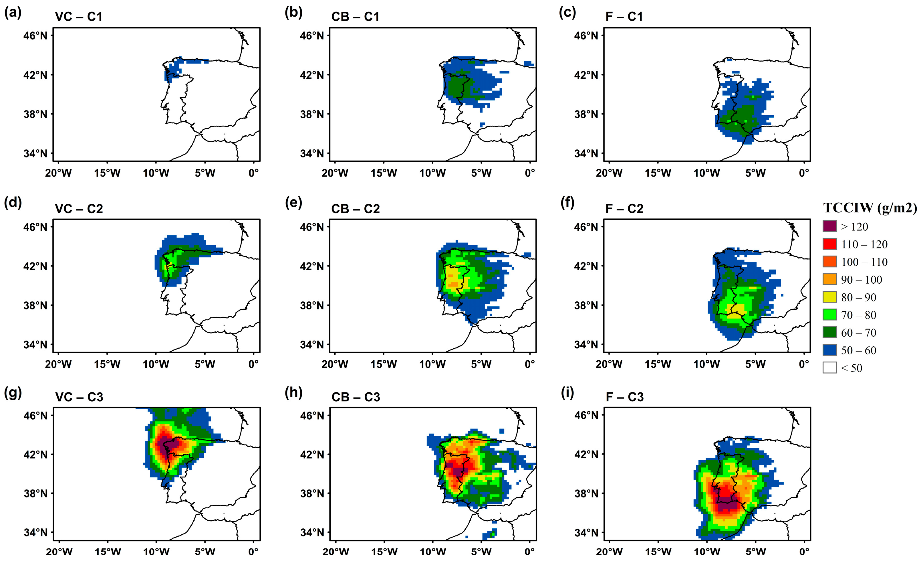
Ice particles comprise a large fraction of convective cloud systems, and ice melting is a key process in the precipitation associated with these systems [62]. Therefore, an analysis of ice cloud formation was performed for the precipitation classes C1, C2, and C3 (Figure 9). Figure 9 clearly shows a relationship between the amount of cloud ice and the amount of precipitation. For C1 events, the lowest values of TTCIW are observed, reaching up to 60 g m−2 for VC, and 70 g m−2 for CB and F. For class C2, an increase in the TCCIW for the three WSs is noticeable, with values reaching 100 g m−2 in CB, and 90 g m−2 for VC and F. Finally, for class C3 (SHHP events), the highest values of TCCIW are visible in VC, concentrated in northwest IP, exceeding 120 g m−2. For CB, the level of ice formation is higher in the northern and central regions, with the maxima in the central region; meanwhile, for F events, there is a higher concentration of TCCIW in the southern region of Portugal, with values higher than 120 g m−2. These results show that the presence of a greater amount of cloud ice is associated with SHHP events.
Relatively to the TCCLW (Figure S10), high values (>250 g m−2) are found for both C2 and C3 events, close to the corresponding meteorological station. For the C3 events in the southern region, the values of TCCLW are higher than for the other classes. Moreover, for C1 events, the amount of cloud liquid water is lower (TCCLW < 200 g m−2).
4. Discussion
This study aims to identify the main dynamic and thermodynamic drivers of the SHHP events associated with regional low-pressure systems. This objective is achieved by analysing the patterns of various atmospheric variables, based on ERA5 reanalysis, for the SHHP events. However, despite improvements in data assimilation systems and NWP models in recent years, several challenges remain. These issues comprise the treatment of model bias, background-error statistics, satellite observation operators, representativeness errors of observations, model processes, and 4D-Var tangent-linear physics, among others [35,63]. Moreover, the resolution of ERA5 is insufficient to resolve the convective scale. These limitations can explain the underestimation of heavy precipitation at sub-hourly scales found in our study. At daily scales, Hénin et al. [56] also documented the underestimation of ERA5 heavy precipitation.
Previous studies have shown that several ingredients must be combined to generate deep convection and heavy precipitation. These ingredients comprise buoyant instability, high moisture content in the low or middle troposphere, and a source of lift [64,65]. Our study confirms the presence of all these ingredients (see, for instance, Figure S11). However, their relative contributions are difficult to assess, particularly considering that we are studying a large number of events. This analysis might be more feasible for isolated events, an area that lies outside of the scope of the present study. It is also interesting to note that previous studies state that synoptic-scale upward motion contributes to the destabilization of the atmosphere but may be too weak to trigger deep convection [64,65]. According to these authors, other sources of lift must be present, specifically, due to mesoscale processes, such as orographic forcing, differential heating, gust fronts, or convergence lines associated with the sea breeze. However, ERA5 is not suitable for assessing these sources of lift. Therefore, in the future, it is important to explore other NWP models, namely, non-hydrostatic limited-area models with grid spacing of the order of 1.5–2.5 km.
5. Conclusions
Multiple studies have been carried out in mainland Portugal with the aim of understanding, quantifying, and previewing different extreme precipitation events [19,25,26,66,67,68]. However, these studies present a view of the mechanisms that may be behind the genesis of this type of event at synoptic and global scales. Furthermore, most studies supporting these results are based on monthly or daily time scales. As such, there is a gap in terms of studies on smaller and shorter scales. Recently, Santos and Belo Pereira [10] analysed sub-hourly heavy precipitation (SHHP) events in mainland Portugal for the period from 2000 to 2020, revealing two main synoptic-scale weather types generating heavy precipitation events. The present study examines in greater depth the dynamic and thermodynamic drivers of sub-hourly precipitation extremes linked to regional low-pressure systems in mainland Portugal, following the sequence of a previous study [10].
Our study reveals that southern Portugal exhibits higher variability in sub-hourly precipitation, with a higher ratio of extreme events on fewer rainy days. The analysis of the various drivers indicates that these SHHP events are associated with low-pressure systems located just to the west of the Iberian Peninsula. These systems are characterised by a positive vorticity core, which is stronger in the upper troposphere and extends downward to low levels. These systems depict a cold core, with higher intensity in the middle troposphere, suggesting that some of these events may be associated with cut-off lows. However, this hypothesis should be validated in a future study, using the criteria defined by Nieto et al. [31].
These systems promote positive vorticity advection in the upper and middle levels (increasing with height), thereby favouring rising motion to the east of the low systems (over western Iberia). Moreover, at low levels, these low-pressure systems promote moisture advection from the Atlantic towards western Iberia (Figure S2), highlighted by the positive anomalies of 2 m dew point temperatures. The cold core in middle levels and low-level moisture advection favour unstable conditions, which were confirmed by the instability indices (CAPE, TT, K-index). Moreover, these events are associated with low CIN values in comparison to other situations. This suggests that a weak or moderate upward motion may be enough to trigger convection. The combination of these conditions promotes the development of deep convective clouds and heavy precipitation. Finally, the total column cloud ice water reveals higher values for heavier precipitation events, suggesting that it may be a useful predictor of heavy precipitation events. The results also showed that the position of these low-pressure systems modulates the region where these heavy precipitation events would occur. All of the aforementioned driving factors for the occurrence of SHHPs tend to act coherently and synergistically.
Although the CAPE values associated with SHHP events appear to be modest (<350 J kg−1), it is important to highlight that, in ERA5, the virtual temperature correction [69] is not applied, which may lead to some underestimation. In the near future, other versions of CAPE and CIN will be tested, namely, mixed-layer and most unstable versions using the virtual potential temperature instead of the equivalent potential temperature, to account for the virtual temperature correction, as used in the current operational version of the ECMWF analyses and forecasts.
SHHP events represent a significant natural hazard, frequently causing significant losses over a wide range of natural systems and socioeconomic sectors in Portugal, such as in agriculture (e.g., viticulture). This study provides a preliminary identification of the main dynamic and thermodynamic drivers of the SHHP events associated with RegL systems, also providing a systematised and comprehensive assessment of the forcing atmospheric conditions, thus paving the way for future improvements in operational forecasts and a resultant risk reduction. In forthcoming research, forecasts of numerical weather prediction (NWP) models can be used for case study events, with the aim of contributing to the optimisation of current forecasts.
Supplementary Materials
The following supporting information can be downloaded at: https://www.mdpi.com/article/10.3390/atmos14091443/s1, Table S1. List of the 34 selected weather stations (WSs) in mainland Portugal. Their codes and names are shown. The corresponding percentages of missing values on the daily timescale precipitation over the recording period are also provided. Table S2. Number and percentage of events recorded in each station and by precipitation class. Figure S1. Composites of hourly anomalies of MSLP (in hPa) (shading) and Z500 (in gpm) (contour lines represented in green, with a spacing of 25 gpm) for (a–c) C1, (d–f) C2, and (g–i) C3. Figure S2. Hourly composites of total column water vapour (TCWV, shading in mm) for precipitation classes (a–c) C0, (d–f) C1, (g–i) C2, and (j–l) C3 in each WS (VC, CB, and F). Figure S3. Composites of hourly anomalies of temperature anomalies (in °C) for precipitation class C3 (SHHP events), at different vertical levels, and for (a) VC, (b) CB, and (c) F. Figure S4. (a) Meridional and (b) zonal cross-sections of relative vorticity composites of hourly anomalies (shading in s−1) and omega vertical velocity (contours in Pa s−1, positive/negative values in solid/dashed lines) for class C3 and CB. Figure S5. (a) Meridional and (b) zonal cross-sections of relative vorticity composites of hourly anomalies (shading in s−1) and omega vertical velocity (contours in Pa s−1, positive/negative values in solid/dashed lines) for class C3 and F. Figure S6. Hourly composites of MSLP (shading in hPa) and position of meridional and zonal cross-sections (white dashed lines) for precipitation class C3 (SHHP events), for (a) VC, (b) CB, and (c) F. Figure S7. Hourly composites of CAPE (shading in J kg−1) and Total-Totals index (blue contours in °C, 2 °C spacing), for (a–c) C0, (d–f) C1, (g–i) C2 (j–l), and C3 in each WS (VC, CB, and F). Figure S8. Hourly composites of convective inhibition (CIN, shading in J kg−1) for precipitation classes (a–c) C0, (d–f) C1, (g–i) C2, and (j–l) C3 in each WS (VC, CB, and F). Figure S9. Hourly composites of K-index (shading in °C) for (a–c) C0, (d–f) C1, (g–i) C2 (j–l), and C3 in each WS (VC, CB, and F). Figure S10. Hourly composites of total column cloud liquid water, TCCLW (shading in g m−2) for precipitation classes (a–c) C1, (d–f) C2, and (g–i) C3 in each WS (VC, CB, and F). Figure S11. Boxplots of (a) CAPE (in J kg−1), (b) CIN (in J kg−1), (c) K-index (in °C), (d) TT-index (in °C), (e) TCWV (in mm), and (f) vertical velocity 700 hPa (in Pa s−1) for precipitation events C3 in each WS (VC, CB, and F).
Author Contributions
Conceptualization, J.A.S., M.B.-P. and J.C.; methodology, J.A.S. and J.C.; software, J.C. and A.F.; validation, all authors; formal analysis, all authors; investigation, all authors; resources, J.A.S.; data curation, J.C.; writing—original draft preparation, J.C.; writing—review and editing, all authors; visualization, all authors; supervision, J.A.S. and A.F.; project administration, J.A.S.; funding acquisition, J.A.S. All authors have read and agreed to the published version of the manuscript.
Funding
Vine & Wine Portugal—Driving Sustainable Growth Through Smart Innovation, PRR & NextGeneration EU, Agendas Mobilizadoras para a Reindustrialização, Contract Nb. C644866286-011.
Institutional Review Board Statement
Not applicable.
Informed Consent Statement
Not applicable.
Data Availability Statement
Data are available upon request.
Acknowledgments
This work is supported by National Funds from FCT—the Portuguese Foundation for Science and Technology, under the project UIDB/04033/2020 and LA/P/0126/2020. We also would like to thank the editor and the three anonymous reviewers for their very useful contributions.
Conflicts of Interest
The authors declare no conflict of interest.
References
- Nielsen, E.R.; Schumacher, R.S. Dynamical insights into extreme short-term precipitation associated with supercells and mesovortices. J. Atmos. Sci. 2018, 75, 2983–3009. [Google Scholar] [CrossRef]
- Fragoso, M.; Trigo, R.M.; Pinto, J.G.; Lopes, S.; Lopes, A.; Ulbrich, S.; Magro, C. The 20 February 2010 Madeira flash-floods: Synoptic analysis and extreme rainfall assessment. Nat. Hazards Earth Syst. Sci. 2012, 12, 715–730. [Google Scholar] [CrossRef]
- Fernández-Nóvoa, D.; González-Cao, J.; Figueira, J.R.; Catita, C.; García-Feal, O.; Gómez-Gesteira, M.; Trigo, R.M. Numerical simulation of the deadliest flood event of Portugal: Unravelling the causes of the disaster. Sci. Total Environ. 2023, 896, 165092. [Google Scholar] [CrossRef] [PubMed]
- Trigo, R.M.; Ramos, C.; Pereira, S.S.; Ramos, A.M.; Zêzere, J.L.; Liberato, M.L.R. The deadliest storm of the 20th century striking Portugal: Flood impacts and atmospheric circulation. J. Hydrol. 2016, 541, 597–610. [Google Scholar] [CrossRef]
- Deierling, W.; Petersen, W.A.; Latham, J.; Ellis, S.; Christian, H.J. The relationship between lightning activity and ice fluxes in thunderstorms. J. Geophys. Res. Atmos. 2008, 113, D15210. [Google Scholar] [CrossRef]
- Petrucci, O.; Aceto, L.; Bianchi, C.; Bigot, V.; Brázdil, R.; Pereira, S.; Kahraman, A.; Kiliç, Ö.; Kotroni, V.; Llasat, M.C.; et al. Flood fatalities in Europe, 1980-2018: Variability, features, and lessons to learn. Water 2019, 11, 1682. [Google Scholar] [CrossRef]
- Gaume, E.; Bain, V.; Bernardara, P.; Newinger, O.; Barbuc, M.; Bateman, A.; Blaškovičová, L.; Blöschl, G.; Borga, M.; Dumitrescu, A.; et al. A compilation of data on European flash floods. J. Hydrol. 2009, 367, 70–78. [Google Scholar] [CrossRef]
- Rochette, S.M.; Moore, J.T. Initiation of an elevated mesoscale convective system associated with heavy rainfall. Weather Forecast. 1996, 11, 443–457. [Google Scholar] [CrossRef]
- Mahale, V.N.; Zhang, G.; Xue, M. Characterization of the 14 June 2011 Norman, Oklahoma, downburst through dual-polarization radar observations and hydrometeor classification. J. Appl. Meteorol. Climatol. 2016, 55, 2635–2655. [Google Scholar] [CrossRef]
- Santos, J.A.; Belo-Pereira, M. Sub-Hourly Precipitation Extremes in Mainland Portugal and Their Driving Mechanisms. Climate 2022, 10, 28. [Google Scholar] [CrossRef]
- Mathias, L.; Ermert, V.; Kelemen, F.D.; Ludwig, P.; Pinto, J.G. Synoptic analysis and hindcast of an intense bow echo in western Europe: The 9 June 2014 storm. Weather Forecast. 2017, 32, 1121–1141. [Google Scholar] [CrossRef]
- Pinto, P.; Belo-Pereira, M. Damaging convective and non-convective winds in Southwestern Iberia during windstorm xola. Atmosphere 2020, 11, 692. [Google Scholar] [CrossRef]
- Skamarock, W.C. Evaluating mesoscale NWP models using kinetic energy spectra. Mon. Weather Rev. 2004, 132, 3019–3032. [Google Scholar] [CrossRef]
- Pereira, S.C.; Carvalho, D.; Rocha, A. Temperature and precipitation extremes over the iberian peninsula under climate change scenarios: A review. Climate 2021, 9, 139. [Google Scholar] [CrossRef]
- North, R.; Trueman, M.; Mittermaier, M.; Rodwell, M.J. An assessment of the SEEPS and SEDI metrics for the verification of 6h forecast precipitation accumulations. Meteorol. Appl. 2013, 20, 164–175. [Google Scholar] [CrossRef]
- Santos, J.A.; Belo-Pereira, M. A comprehensive analysis of hail events in Portugal: Climatology and consistency with atmospheric circulation. Int. J. Climatol. 2019, 39, 188–205. [Google Scholar] [CrossRef]
- Sousa, J.F.; Fragoso, M.; Mendes, S.; Corte-Real, J.; Santos, J.A. Statistical-dynamical modeling of the cloud-to-ground lightning activity in Portugal. Atmos. Res. 2013, 132–133, 46–64. [Google Scholar] [CrossRef]
- Peel, M.C.; Finlayson, B.L.; McMahon, T.A. Updated world map of the Köppen-Geiger climate classification. Hydrol. Earth Syst. Sci. 2007, 11, 1633–1644. [Google Scholar] [CrossRef]
- Trıgo, R.M.; Da Câmara, C.C. Circulation weather types and their influence on the precipitatıon regime in Portugal. Int. J. Climatol. 2000, 20, 1559–1581. [Google Scholar] [CrossRef]
- Hoinka, K.P.; De Castro, M. The Iberian Peninsula thermal low. Q. J. R. Meteorol. Soc. 2003, 129, 1491–1511. [Google Scholar] [CrossRef]
- Amorim Ferreira, H. Characterisation of air masses over Portugal. In Memórias do Serviço Meteorológico 35; Serviço Meteorologico de Angola: Lisbon, Portugal, 1954. [Google Scholar]
- Woollings, T.; Pinto, J.G.; Santos, J.A. Dynamical evolution of North Atlantic ridges and Poleward Jet stream displacements. J. Atmos. Sci. 2011, 68, 954–963. [Google Scholar] [CrossRef]
- Santos, J.A.; Woollings, T.; Pinto, J.G. Are the winters 2010 and 2012 archetypes exhibiting extreme opposite behavior of the north atlantic jet stream. Mon. Weather Rev. 2013, 141, 3626–3640. [Google Scholar] [CrossRef]
- Nieto, R.; Gimeno, L.; Añel, J.A.; De la Torre, L.; Gallego, D.; Barriopedro, D.; Gallego, M.; Gordillo, A.; Redaño, A.; Delgado, G. Analysis of the precipitation and cloudiness associated with COLs occurrence in the Iberian Peninsula. Meteorol. Atmos. Phys. 2007, 96, 103–119. [Google Scholar] [CrossRef]
- Belo-Pereira, M.; Dutra, E.; Viterbo, P. Evaluation of global precipitation data sets over the Iberian Peninsula. J. Geophys. Res. Atmos. 2011, 116, D20101. [Google Scholar] [CrossRef]
- Soares, P.M.M.; Cardoso, R.M.; Miranda, P.M.A.; de Medeiros, J.; Belo-Pereira, M.; Espirito-Santo, F. WRF high resolution dynamical downscaling of ERA-Interim for Portugal. Clim. Dyn. 2012, 39, 2497–2522. [Google Scholar] [CrossRef]
- Van Delden, A. The synoptic setting of thunderstorms in Western Europe. Atmos. Res. 2001, 56, 89–110. [Google Scholar] [CrossRef]
- Peppler, R.A.; Lamb, P.J. Tropospheric Static Stability and Central North American Growing Season Rainfall. Mon. Weather Rev. 1989, 117, 1156–1180. [Google Scholar] [CrossRef]
- Meyer, J.; Neuper, M.; Mathias, L.; Zehe, E.; Pfister, L. Atmospheric conditions favouring extreme precipitation and flash floods in temperate regions of Europe. Hydrol. Earth Syst. Sci. 2022, 26, 6163–6183. [Google Scholar] [CrossRef]
- Junker, N.W.; Schneider, R.S.; Fauver, S.L. A study of heavy rainfall events during the great midwest flood of 1993. Weather Forecast. 1999, 14, 701–712. [Google Scholar] [CrossRef]
- Nieto, R.; Gimeno, L.; de La Torre, L.; Ribera, P.; Gallego, D.; García-Herrera, R.; García, J.A.; Nuñez, M.; Redaño, A.; Lorente, J. Climatological features of cutoff low systems in the Northern Hemisphere. J. Clim. 2005, 18, 3085–3103. [Google Scholar] [CrossRef]
- Ferreira, R.N. Cut-off lows and extreme precipitation in eastern spain: Current and future climate. Atmosphere 2021, 12, 835. [Google Scholar] [CrossRef]
- Santos, M.; Fragoso, M.; Santos, J.A. Regionalization and susceptibility assessment to daily precipitation extremes in mainland Portugal. Appl. Geogr. 2017, 86, 128–138. [Google Scholar] [CrossRef]
- Hersbach, H.; Bell, B.; Berrisford, P.; Hirahara, S.; Horányi, A.; Muñoz-Sabater, J.; Nicolas, J.; Peubey, C.; Radu, R.; Schepers, D.; et al. The ERA5 global reanalysis. Q. J. R. Meteorol. Soc. 2020, 146, 1999–2049. [Google Scholar] [CrossRef]
- Hacker, J.; Draper, C.; Madaus, L. Challenges and opportunities for data assimilation in mountainous environments. Atmosphere 2018, 9, 127. [Google Scholar] [CrossRef]
- Hersbach, H.; Bell, B.; Berrisford, P.; Biavati, G.; Horányi, A.; Muñoz Sabater, J.; Nicolas, J.; Peubey, C.; Radu, R.; Rozum, I.; et al. ERA5 Hourly Data on Single Levels from 1940 to Present. Available online: https://cds.climate.copernicus.eu/cdsapp#!/dataset/reanalysis-era5-single-levels?tab=overview (accessed on 18 May 2023).
- Hersbach, H.; Bell, B.; Berrisford, P.; Biavati, G.; Horányi, A.; Muñoz Sabater, J.; Nicolas, J.; Peubey, C.; Radu, R.; Rozum, I.; et al. ERA5 Hourly Data on Pressure Levels from 1940 to Present. Available online: https://cds.climate.copernicus.eu/cdsapp#!/dataset/reanalysis-era5-pressure-levels?tab=overview (accessed on 18 May 2023).
- Kunz, M. The skill of convective parameters and indices to predict isolated and severe thunderstorms. Nat. Hazards Earth Syst. Sci. 2007, 7, 327–342. [Google Scholar] [CrossRef]
- Belo-Pereira, M.; Andrade, C.; Pinto, P. A long-lived tornado on 7 December 2010 in mainland Portugal. Atmos. Res. 2017, 185, 202–215. [Google Scholar] [CrossRef]
- DeRubertis, D. Recent trends in four common stability indices derived from US radiosonde observations. J. Clim. 2006, 19, 309–323. [Google Scholar] [CrossRef]
- Kirkpatrick, C.; McCaul, E.W.; Cohen, C. Variability of updraft and downdraft characteristics in a large parameter space study of convective storms. Mon. Weather Rev. 2009, 137, 1550–1561. [Google Scholar] [CrossRef]
- Bluestein, H.B.; Jain, M.H. Formation of mesoscale lines of pirecipitation: Severe squall lines in Oklahoma during the spring. J. Atmos. Sci. 1985, 42, 1711–1732. [Google Scholar] [CrossRef]
- Rochette, S.M.; Moore, J.T.; Market, P.S. The importance of parcel choice in elevated CAPE computations. Natl. Wea. Dig. 1999, 23, 20–32. [Google Scholar]
- Blanchard, D.O. Assessing the vertical distribution of convective available potential energy. Weather Forecast. 1998, 13, 870–877. [Google Scholar] [CrossRef]
- López, L.; Marcos, J.L.; Sanchez, J.L.; Castro, A.; Fraile, R. CAPE values and hailstorms on northwestern Spain. Atmos. Res. 2001, 56, 147–160. [Google Scholar] [CrossRef]
- Kaltenböck, R.; Diendorfer, G.; Dotzek, N. Evaluation of thunderstorm indices from ECMWF analyses, lightning data and severe storm reports. Atmos. Res. 2009, 93, 381–396. [Google Scholar] [CrossRef]
- González-Rojí, S.J.; Carreno-Madinabeitia, S.; Sáenz, J.; Ibarra-Berastegi, G. Changes in the simulation of instability indices over the Iberian Peninsula due to the use of 3DVAR data assimilation. Hydrol. Earth Syst. Sci. Discuss. 2020, 2020, 1–25. [Google Scholar]
- Groenemeijer, P.; Púčik, T.; Tsonevsky, I.; Bechtold, P. An Overview of Convective Available Potential Energy and Convective Inhibition Provided by NWP Models for Operational Forecasting; ECMWF Technical Memoranda; ECMWF: Reading, UK, 2019; pp. 1–19. [Google Scholar]
- Lock, N.A.; Houston, A.L. Empirical examination of the factors regulating thunderstorm initiation. Mon. Weather Rev. 2014, 142, 240–258. [Google Scholar] [CrossRef]
- Owens, R.; Hewson, T. ECMWF Forecast User Guide; ECMWF: Reading, UK, 2018. [Google Scholar]
- Siedlecki, M. Selected instability indices in Europe. Theor. Appl. Climatol. 2009, 96, 85–94. [Google Scholar] [CrossRef]
- Iturrioz, I.; Hernández, E.; Ribera, P.; Queralt, S. Instability and its relation to precipitation over the Eastern Iberian Peninsula. Adv. Geosci. 2007, 10, 45–50. [Google Scholar] [CrossRef]
- Letestu, S. International Meteorological Tables; World Meteor Organization: Geneva, Switzerland, 1966. [Google Scholar]
- Santos, J.A.; Corte-Real, J.; Leite, S.M. Weather regimes and their connection to the winter rainfall in Portugal. Int. J. Climatol. 2005, 25, 33–50. [Google Scholar] [CrossRef]
- Yun, B.I.; Rim, K.S. Construction of Lanczos type filters for the Fourier series approximation. Appl. Numer. Math. 2009, 59, 280–300. [Google Scholar] [CrossRef]
- Hénin, R.; Liberato, M.L.R.; Ramos, A.M.; Gouveia, C.M. Assessing the use of satellite-based estimates and high-resolution precipitation datasets for the study of extreme precipitation events over the Iberian Peninsula. Water 2018, 10, 1688. [Google Scholar] [CrossRef]
- Durran, D.R.; Snellman, L.W. The diagnosis of synoptic-scale vertical motion in an operational environment. Weather Forecast. 1987, 2, 17–31. [Google Scholar] [CrossRef]
- Hoskins, B.; Pedder, M.; Jones, D.W. The omega equation and potential vorticity. Q. J. R. Meteorol. Soc. A J. Atmos. Sci. Appl. Meteorol. Phys. Oceanogr. 2003, 129, 3277–3303. [Google Scholar] [CrossRef]
- He, C. Future Drying Subtropical East Asia in Winter: Mechanism and Observational Constraint. J. Clim. 2023, 36, 2985–2998. [Google Scholar] [CrossRef]
- Palmén, E.; Newton, C.W. Atmospheric Circulation Systems: Their Structure and Physical Interpretation; Academic Press: Cambridge, MA, USA, 1969; ISBN 0125445504. [Google Scholar]
- Winkler, R.; Zwatz-Meise, V. Manual of Synoptic Satellite Meteorology; Concept. Model. Vers. 6; 2001. Available online: http://www.zamg.ac.at/docu/Manual/SatManu/main.htm (accessed on 23 July 2023).
- Bringi, V.N.; Chandrasekar, V. Polarimetric Doppler Weather Radar: Principles and Applications; Cambridge University Press: Cambridge, UK, 2001; ISBN 0521623847. [Google Scholar]
- Hu, G.; Dance, S.L.; Bannister, R.N.; Chipilski, H.G.; Guillet, O.; Macpherson, B.; Weissmann, M.; Yussouf, N. Progress, challenges, and future steps in data assimilation for convection-permitting numerical weather prediction: Report on the virtual meeting held on 10 and 12 November 2021. Atmos. Sci. Lett. 2023, 24, e1130. [Google Scholar] [CrossRef]
- McNulty, R.P. Severe and convective weather: A central region forecasting challenge. Weather Forecast. 1995, 10, 187–202. [Google Scholar] [CrossRef]
- Doswell, C.A.; Brooks, H.E.; Maddox, R.A. Flash flood forecasting: An ingredients-based methodology. Weather Forecast. 1996, 11, 560–581. [Google Scholar] [CrossRef]
- Ramos, A.M.; Trigo, R.M.; Liberato, M.L.R. A ranking of high-resolution daily precipitation extreme events for the Iberian Peninsula. Atmos. Sci. Lett. 2014, 15, 328–334. [Google Scholar] [CrossRef]
- Durao, R.M.; Pereira, M.J.; Costa, A.C.; Delgado, J.; Del Barrio, G.; Soares, A. Spatial–temporal dynamics of precipitation extremes in southern Portugal: A geostatistical assessment study. Int. J. Climatol. 2010, 30, 1526–1537. [Google Scholar] [CrossRef]
- Santos, M.; Fonseca, A.; Fragoso, M.; Santos, J.A. Recent and future changes of precipitation extremes in mainland Portugal. Theor. Appl. Climatol. 2019, 137, 1305–1319. [Google Scholar] [CrossRef]
- Doswell, C.A., III; Rasmussen, E.N. The effect of neglecting the virtual temperature correction on CAPE calculations. Weather Forecast. 1994, 9, 625–629. [Google Scholar] [CrossRef]
Figure 1.
(a) Hypsometric map of mainland Portugal (elevation in m), with three weather stations (VC, CB, and F) with sub-hourly data (timescale of 10 min, 2000–2022) used in the calculation of the different classes of precipitation (C0–3). (b) Bar chart of the number of events recorded in each station and by precipitation class. (c) Bar chart of the percentage of events over the total number of precipitation records in each station and by precipitation class. (d) Spatial distribution of the Pearson correlation coefficients between daily precipitation in the three main weather stations (VC, CB, and F), excluding days without precipitation, and the remaining weather stations (see legend).
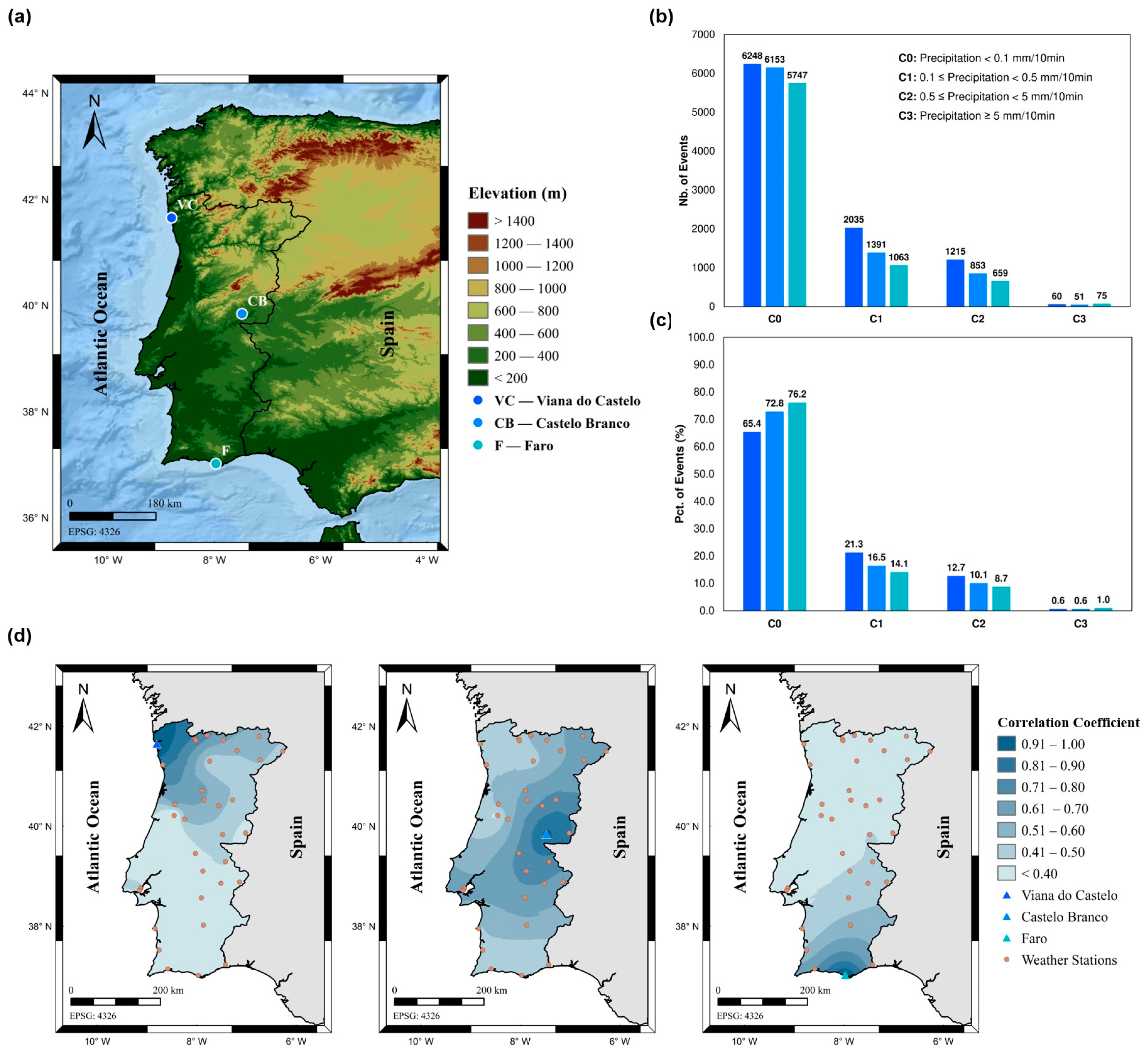
Figure 2.
The 50th and 99th percentile (p50 and p99) of hourly ERA5: (a–c) total precipitation for p50, (d–f) convective precipitation for p50, (g–i) total precipitation for p99, (j–l) convective precipitation for p99, for the SHHP events (C3 class) in each WS (VC, CB, and F), and (m–o) quantile–quantile plot for all events of the precipitation (hourly) in each WS (VC, CB, and F); black line: reference line; red dotted line: tendency; blue dots: precipitation data (ERA5 vs. OBS).
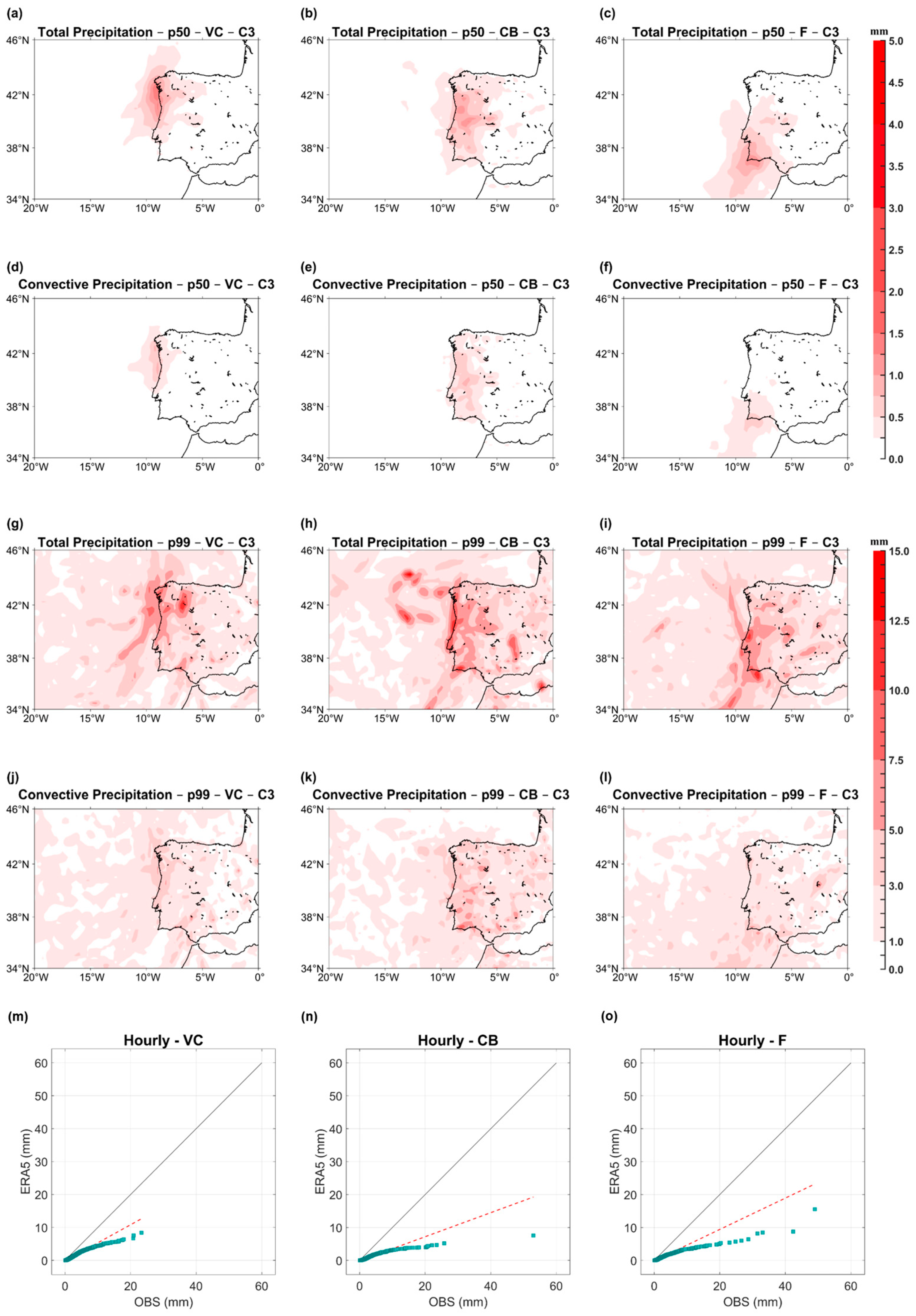
Figure 3.
Hourly composites of MSLP (in hPa) (shading) and Z500 (in gpm) (contour lines represented in blue, with a spacing of 50 gpm) for (a–c) C0, (d–f) C1, (g–i) C2 (j–l), and C3.
Figure 3.
Hourly composites of MSLP (in hPa) (shading) and Z500 (in gpm) (contour lines represented in blue, with a spacing of 50 gpm) for (a–c) C0, (d–f) C1, (g–i) C2 (j–l), and C3.
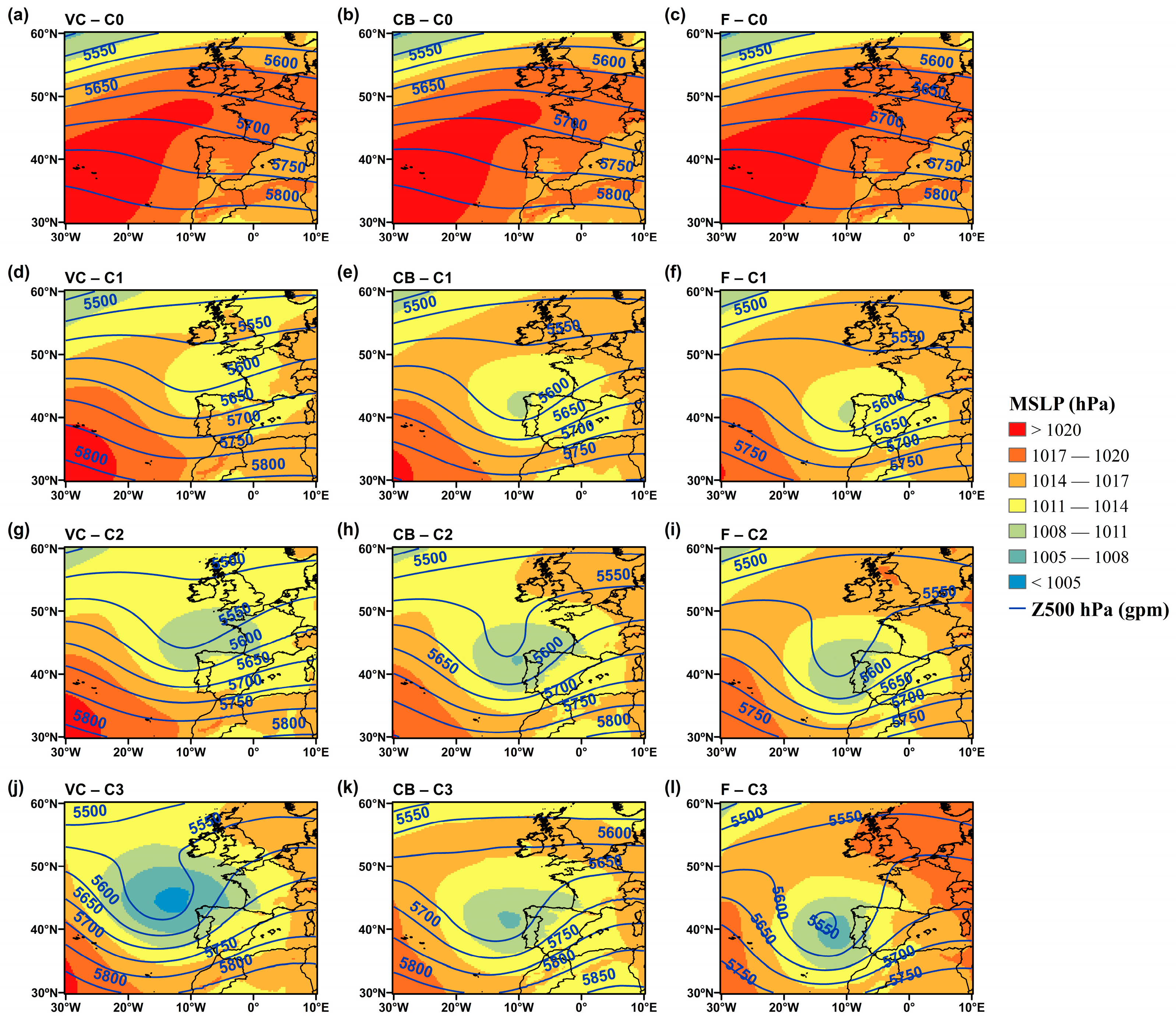
Figure 4.
Composites of hourly anomalies of (a–c) MSLP (in hPa), (d–f) temperature 500 hPa (in °C), (g–i) 2 m temperature (in °C), (j–l) 2 m dew point temperature (shading in °C), and 10 m wind vector (black arrows in m s−1) for the SHHP events (C3 precipitation class) in the three selected WSs (VC, CB, and F).
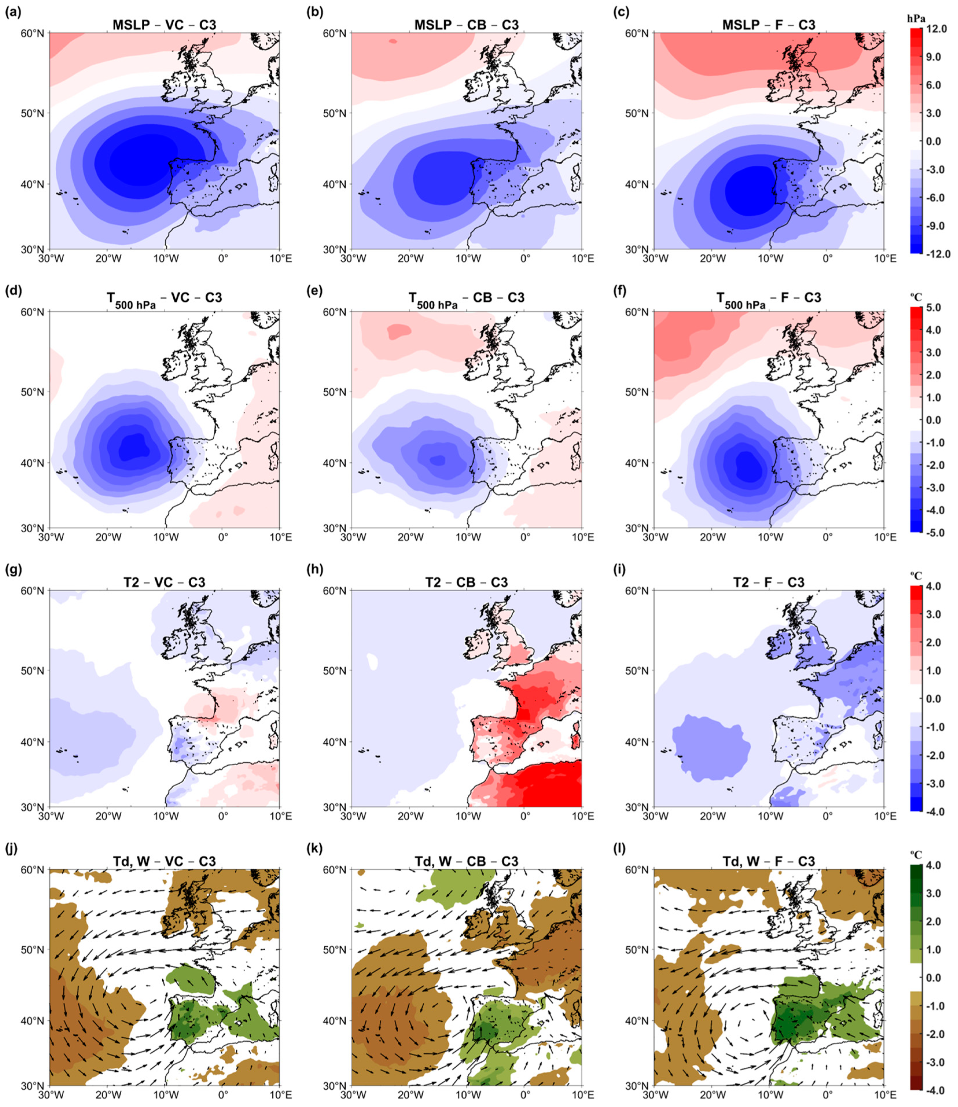
Figure 5.
Composites of hourly anomalies of geopotential anomalies (in gpm) for precipitation class C3 (SHHP events), at different vertical pressure levels, and for (a) VC, (b) CB, and (c) F.
Figure 5.
Composites of hourly anomalies of geopotential anomalies (in gpm) for precipitation class C3 (SHHP events), at different vertical pressure levels, and for (a) VC, (b) CB, and (c) F.

Figure 6.
Composites of hourly anomalies of the potential temperature anomaly (in °C) for precipitation class C3 (SHHP events), at different vertical levels, and for (a) VC, (b) CB, and (c) F.
Figure 6.
Composites of hourly anomalies of the potential temperature anomaly (in °C) for precipitation class C3 (SHHP events), at different vertical levels, and for (a) VC, (b) CB, and (c) F.
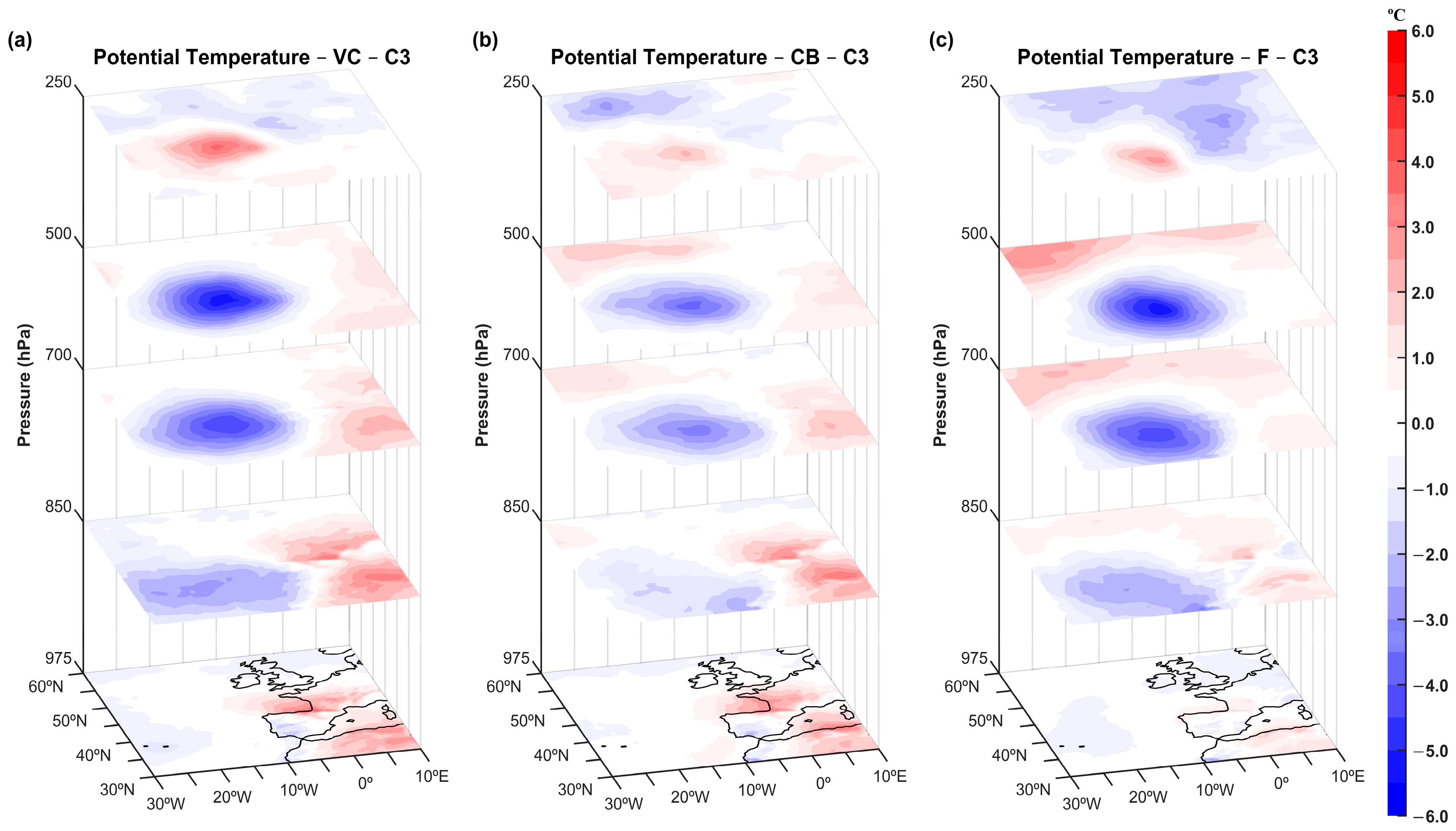
Figure 7.
(a) Meridional and (b) zonal cross-sections of the relative vorticity composites of hourly anomalies (shading in s−1) and omega vertical velocity (contours in Pa s−1, positive/negative values in solid/dashed lines, respectively) for class C3 and VC.
Figure 7.
(a) Meridional and (b) zonal cross-sections of the relative vorticity composites of hourly anomalies (shading in s−1) and omega vertical velocity (contours in Pa s−1, positive/negative values in solid/dashed lines, respectively) for class C3 and VC.

Figure 8.
Composites of hourly atmospheric instability indices: (a–c) CAPE (shading in J kg−1) and the total totals index (blue contours in °C, 2 °C spacing), (d–f) the K-index (in °C). and (g–i) CIN (in J kg−1) for SHHP events (C3) in each WS (VC, CB, and F).
Figure 8.
Composites of hourly atmospheric instability indices: (a–c) CAPE (shading in J kg−1) and the total totals index (blue contours in °C, 2 °C spacing), (d–f) the K-index (in °C). and (g–i) CIN (in J kg−1) for SHHP events (C3) in each WS (VC, CB, and F).
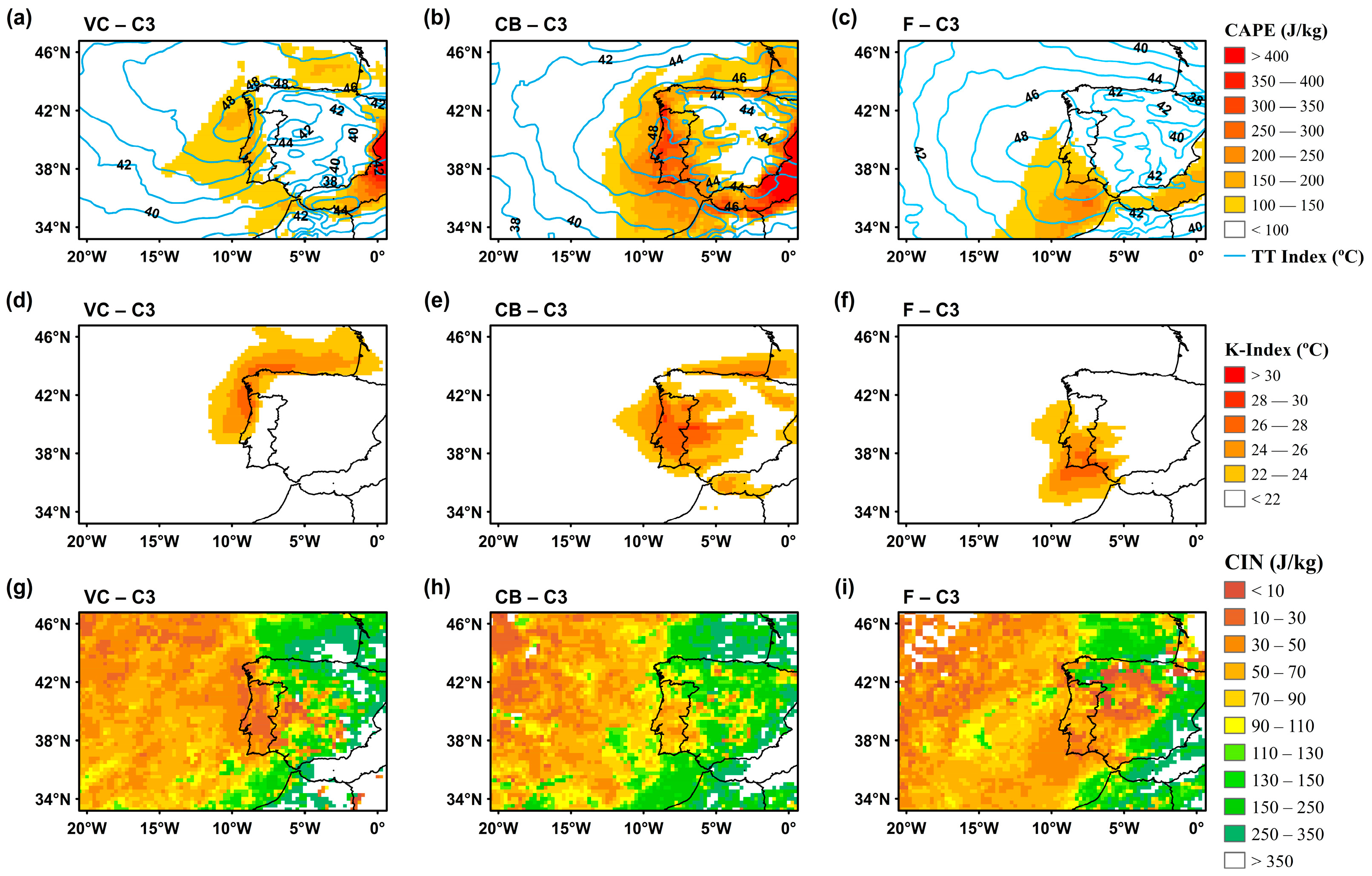
Figure 9.
Hourly composites of total column cloud ice water, TCCIW (shading in g m−2) for precipitation classes (a–c) C1, (d–f) C2, and (g–i) C3 in each WS (VC, CB, and F).
Figure 9.
Hourly composites of total column cloud ice water, TCCIW (shading in g m−2) for precipitation classes (a–c) C1, (d–f) C2, and (g–i) C3 in each WS (VC, CB, and F).
Disclaimer/Publisher’s Note: The statements, opinions and data contained in all publications are solely those of the individual author(s) and contributor(s) and not of MDPI and/or the editor(s). MDPI and/or the editor(s) disclaim responsibility for any injury to people or property resulting from any ideas, methods, instructions or products referred to in the content. |
© 2023 by the authors. Licensee MDPI, Basel, Switzerland. This article is an open access article distributed under the terms and conditions of the Creative Commons Attribution (CC BY) license (https://creativecommons.org/licenses/by/4.0/).
Share and Cite
MDPI and ACS Style
Cruz, J.; Belo-Pereira, M.; Fonseca, A.; Santos, J.A. Dynamic and Thermodynamic Drivers of Severe Sub-Hourly Precipitation Events in Mainland Portugal. Atmosphere 2023, 14, 1443. https://doi.org/10.3390/atmos14091443
AMA Style
Cruz J, Belo-Pereira M, Fonseca A, Santos JA. Dynamic and Thermodynamic Drivers of Severe Sub-Hourly Precipitation Events in Mainland Portugal. Atmosphere. 2023; 14(9):1443. https://doi.org/10.3390/atmos14091443
Chicago/Turabian StyleCruz, José, Margarida Belo-Pereira, André Fonseca, and João A. Santos. 2023. "Dynamic and Thermodynamic Drivers of Severe Sub-Hourly Precipitation Events in Mainland Portugal" Atmosphere 14, no. 9: 1443. https://doi.org/10.3390/atmos14091443
Note that from the first issue of 2016, this journal uses article numbers instead of page numbers. See further details here.