Radial Basis Function Method for Predicting the Evolution of Aerosol Size Distributions for Coagulation Problems

Abstract

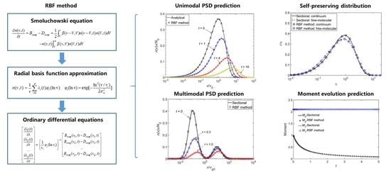
The dynamic evolution of particle size distributions (PSDs) during coagulation is of great importance in many atmospheric and engineering applications. To date, various numerical methods have been developed for solving the general dynamic equation under different scenarios. In this study, a radial basis function (RBF) method was proposed to solve particle coagulation evolution. This method uses a Gaussian function as the basis function to approximate the size distribution function. The original governing equation was then converted to ordinary differential equations (ODEs), along with numerical quadratures. The RBF method was compared with the analytical solutions and sectional method to validate its accuracy. The comparison results showed that the RBF method provided almost accurate predictions of the PSDs for different coagulation kernels. This method was also verified to be reliable in predicting the self-preserving distributions reached over long periods and for describing the temporal evolution of moments. For multimodal coagulation, the RBF method also accurately predicted the temporal evolution of a bimodal distribution owing to scavenging effects. Moreover, the computational times of the RBF method for these cases were usually of the order of seconds. Thus, the RBF method is verified as a reliable and efficient tool for predicting PSD evolution during coagulation.

1. Introduction

The population balance equation (PBE), also known as the general dynamic equation, plays an important role in describing the evolution of particle size distributions for various atmospheric and engineering applications, including the airborne transmission of COVID-19 [1], atmospheric aerosol formation and transport [2,3,4], combustion-generated nanoparticles [5,6], polymerization and crystallization processes [7,8], and nuclear radioactive aerosols [9]. The basic form of the population balance equation originates from the Smoluchowski equation, which describes the temporal evolution of a continuous particle size distribution (PSD) caused by coagulation [10]. Because of complex integral–differential characteristics, various numerical methods have been proposed to solve the PBE. The numerical methods can be categorized into the sectional method [11,12], method of moments [13,14,15], stochastic method [16,17,18], and spectral method [19,20]. These methods are based on different principles and exhibit different accuracies and efficiencies. Detailed comparisons are provided in previous studies [21,22].

Among the existing numerical methods, many assume that the PSD can be described by a specific distribution function, and the parameters of this predefined distribution can be solved using moment equations. The typical distribution patterns include the well-known log-normal distribution [23], the improved log-skew normal distribution [24], the modal aerosol approach [25], and weighted sum of number density functions with a log-normal kernel, gamma kernel, or beta kernel [26,27]. Although these methods achieve moment closure and well predict moments, they generally lack accuracy and stability in predicting the size distribution evolution. This is mainly because the PSD information is missing when transforming the PBE into a finite set of moment equations [28]. Moreover, the predefined distributions are not sufficiently flexible to represent the unsolved particle size distribution.

In recent years, radial basis functions (RBFs) have been extensively applied in solving complex numerical problems involving ordinary differential equations (ODEs), partial differential equations (PDEs), and integral equations [29,30,31]. Moreover, RBFs are popular kernel functions used in neural networks and have many applications in predicting atmospheric pollutant concentrations [32,33,34,35]. The basic principle of RBFs is their superior ability to approximate continuous functions. Therefore, in a previous study, RBFs were adopted to solve the PBE for particle coagulation [36]. The number density function was approximated using two-dimensional Gaussian radial basis functions with volume and time as the variables, which provided an accurate description of PSDs over a period of time but were limited to predicting long time-period, self-preserving distributions. Subsequently, Alzyod and Charton [37] proposed a meshless radial basis method to solve the PBE for particle growth, nucleation, coagulation, and breakage. They used multiquadric basis functions and transformed the PBE into ODEs, and, in another study, proposed an adaptive radial basis method to model the hydrodynamic behavior of liquid–liquid dispersions [38]. However, these method formulations are difficult to use and validations of the method are only for simple coagulation cases, which cannot guarantee the accuracy of the method for more general coagulation problems. Therefore, the RBF methods proposed in previous studies are incomplete and need further improvements and more sufficient validations.

This study further develops a reliable and robust RBF method to solve the PBE for coagulation and provides an adequate validation of the method under various possible coagulation situations. Section 2 presents the theory and numerical details of the method. The governing equations were derived based on the radial basis function approximation. The integral terms were obtained using the Gaussian quadrature, along with mathematical treatments that decreased the quadrature error. The final derived equations are a set of ODEs that can be easily solved using commercial ODE solvers. Section 3 validates the RBF method for various coagulation cases, including constant kernel and sum kernel coagulations, realistic Brownian coagulation in the continuum and free-molecular regimes, self-preserving distributions, and multimodal coagulation. The predictions obtained using the RBF method were compared with the analytical solutions and those obtained using a sectional method to validate its accuracy and efficiency. Finally, Section 4 summarizes the content of this study.

2. Materials and Methods

A radial basis function (RBF) is a function whose value changes with the distance from a center point. Typical radial basis functions are the Gaussian, multiquadric, and inverse multiquadric functions. In this section, the theory and numerical procedures of the radial basis function method are presented in detail.

2.1. Governing Equations

For particle coagulation, the governing PBE to describe the time evolution of particle size distributions is expressed in the following integral–differential form:

$$\begin{array}{c}\frac{\partial n(v,t)}{\partial t}=B_{coag}-D_{coag}=\frac{1}{2}{\displaystyle {\int }_0^v\beta (v-\overline{v},\overline{v})}n(v-\overline{v},t)n(\overline{v},t)d\overline{v}\\ -n(v,t){\displaystyle {\int }_0^{\infty }\beta (v,\overline{v})}n(\overline{v},t)d\overline{v}\end{array}$$

(1)

where $n(v,t)$ is the number density function for the particle volume $v$ at time $t$, $B_{coag}$ is the birth term of particles with volume $v$ caused by coagulation, $D_{coag}$ is the death term of particles with volume $v$ caused by coagulation, and $\beta (v,\overline{v})$ is the coagulation kernel for two particles with volumes $v$ and $\overline{v}$, respectively.

The principle of the RBF method is to approximate the number density function $n(v,t)$ using the weighted sum of the radial basis functions. In our previous study [36], both volume $v$ and time $t$ were regarded as the input variables into the two-dimensional Gaussian functions, thereby complicating the solving process. A convenient approach is to use only a one-dimensional Gaussian function for volume $v$ and to make the coefficients time-variant, which can be expressed as follows:

$$n(v,t)=\frac{1}{v}{\displaystyle \sum _{i=1}^p{\lambda }_i(t){\phi }_i(\ln v)}$$

(2)

$${\phi }_i(\ln v)=\exp [-\frac{{\ln }^2(v/v_i)}{2{\sigma }_{vi}^2}]$$

(3)

where ${\lambda }_i(t)$ is the i-th coefficient that changes with time $t$, ${\phi }_i$ is the i-th Gaussian kernel located at the center point $v_i$, and ${\sigma }_{vi}$ is the standard deviation of the i-th Gaussian kernel. It should be noted that the logarithmic transformation from $v$ to $\ln v$ is used in Equations (2) and (3) because aerosol particle sizes are usually distributed on logarithmic scales rather than on linear scales.

In addition to the normal RBF approximations, Equations (2) and (3) also have physical implications. The Gaussian function coupled with the logarithmic transformation is equivalent to the widely used log-normal distribution. Thus, the approximation of $n(v,t)$ in Equations (2) and (3) can be interpreted as the superposition of many log-normal sub-distributions, which is also consistent with the idea of a previous study [39]. Each sub-distribution represents a flexible component; therefore, all sub-distributions have the ability to approximate distributions of any shape.

Substituting Equation (2) into Equation (1) and calculating the derivative yields:

$$\frac{\partial n(v,t)}{\partial t}=\frac{1}{v}{\displaystyle \sum _{i=1}^p\frac{\partial {\lambda }_i(t)}{\partial t}{\phi }_i(\ln v)}=B_{coag}(v,t)-D_{coag}(v,t)$$

(4)

According to the collocation method principle, for any given point $v$, Equation (4) is automatically satisfied. For simplicity and realizability, the collocation points are set to be the same as the center points of the Gaussian kernels. In this case, Equation (4) is transformed into the following p equations:

$$\frac{1}{v_j}{\displaystyle \sum _{i=1}^p\frac{\partial {\lambda }_i(t)}{\partial t}{\phi }_i(\ln v_j)}=B_{coag}(v_j,t)-D_{coag}(v_j,t)$$

(5)

where $j=1,2,\dots ,p$.

Using the matrix representation for Equation (5) leads to the following governing equations for the coefficients ${\lambda }_i(t)$:

$$\left[\begin{array}{c}\frac{\partial {\lambda }_1(t)}{\partial t}\\ \frac{\partial {\lambda }_2(t)}{\partial t}\\ \dots \\ \frac{\partial {\lambda }_p(t)}{\partial t}\end{array}\right]={\left\{\frac{1}{v_i}{\phi }_j(\ln v_i)\right\}}^{-1}\left[\begin{array}{c}{B}_{coag}(v_1,t)-D_{coag}(v_1,t)\\ B_{coag}(v_2,t)-D_{coag}(v_2,t)\\ \dots \\ B_{coag}(v_p,t)-D_{coag}(v_p,t)\end{array}\right]$$

(6)

In Equation (6), the left array represents the time derivatives of ${\lambda }_i(t)$, the first term on the right-hand side is a constant matrix that depends only on the kernel function and selected center points, and the second term is an array of coagulation integrals. The calculations for these integrals are presented in Section 2.2.

The initial conditions for Equation (6) is simply substituting $t=0$ into Equation (2) and using the initial size distribution, as follows:

$$n(v,0)=\frac{1}{v}{\displaystyle \sum _{i=1}^p{\lambda }_i(0){\phi }_i(\ln v)}$$

(7)

By applying the same procedure as that for Equation (6), the initial values of ${\lambda }_i(0)$ can be calculated as follows:

$$\left[\begin{array}{c}{\lambda }_1(0)\\ {\lambda }_2(0)\\ \dots \\ {\lambda }_p(0)\end{array}\right]={\left\{\frac{1}{v_i}{\phi }_j(\ln v_i)\right\}}^{-1}\left[\begin{array}{c}n(v_1,0)\\ n(v_2,0)\\ \dots \\ n(v_p,0)\end{array}\right]$$

(8)

Thus, Equation (6), together with the initial conditions in Equation (8), constitutes the governing equations for ${\lambda }_i(t)$, which is relatively concise compared with the original PBE.

2.2. Quadrature Approximation

For the governing Equation (6), the remaining issue is to calculate the complex integrals for the birth term $B_{coag}$ and death term $D_{coag}$. In our previous study [36], $B_{coag}$ and $D_{coag}$ were calculated using the Gauss–Legendre quadrature and Gauss–Laguerre quadrature, respectively; however, the two quadratures may not accurately predict long-term coagulation, because the integral error increases with time in the long-term. To address this problem, this study adopts special mathematical treatments for the integrals, and the quadrature accuracy can be guaranteed even for long time-period, self-preserving predictions, as illustrated in Section 3.3.

For the birth term $B_{coag}$, the integral domain of $[0,v]$ should be transformed into [–1, 1] to satisfy the Gauss–Legendre quadrature. To achieve this, the transformation $\overline{v}=(u+1)v/2$ is used, and the original integral becomes:

$$\begin{array}{l}{B}_{coag}(v,t)=\frac{1}{2}{\displaystyle {\int }_0^v\beta (v-\overline{v},\overline{v})}n(v-\overline{v},t)n(\overline{v},t)d\overline{v}\\ =\frac{v}{4}{\displaystyle {\int }_{-1}^1\beta (\frac{v}{2}-\frac{v}{2}u,\frac{v}{2}+\frac{v}{2}u)}n(\frac{v}{2}-\frac{v}{2}u,t)n(\frac{v}{2}+\frac{v}{2}u,t)du\end{array}$$

(9)

Applying the Gauss–Legendre quadrature to Equation (9) yields the following final quadrature formula for $B_{coag}$:

$$B_{coag}(v,t)=\frac{v}{4}{\displaystyle \sum _{k=1}^s{w}_k\beta (\frac{v}{2}-\frac{v}{2}{u}_k,\frac{v}{2}+\frac{v}{2}{u}_k)n(\frac{v}{2}-\frac{v}{2}{u}_k,t)n(\frac{v}{2}+\frac{v}{2}{u}_k,t)}$$

(10)

where $u_k$ and $w_k$ are the nodes and weights of the Gauss-Legendre quadrature, respectively, and $s$ is the number of Gauss-Legendre quadrature points. Calculations of the nodes and weights for the quadrature are provided in the literature [40].

For the death term $D_{coag}$, the previous Gauss–Laguerre quadrature is not suitable for long-term coagulation calculations. Thus, the infinite integral interval [0, ∞] is first truncated into a finite interval $[v_{\min },v_{\max }]$, which has a negligible impact on the integral results. Here, $v_{\min }$ is the smallest volume, and $v_{\max }$ is the largest volume of the computation domain. Because the entire particle volume range is relatively large in actual situations, the integral should be calculated under logarithmic scales to decrease the quadrature error; therefore:

$$\begin{array}{l}{D}_{coag}(v,t)=n(v,t){\displaystyle {\int }_{v_{\min }}^{v_{\max }}\beta (v,\overline{v})}n(\overline{v},t)d\overline{v}\\ =n(v,t){\displaystyle {\int }_{\ln v_{\min }}^{\ln v_{\max }}\beta (v,e^x)}n(e^x,t)e^{x}dx(x=\ln \overline{v})\end{array}$$

(11)

To satisfy the Gauss–Legendre quadrature rule, the above integral interval $[\ln v_{\min },\ln v_{\max }]$ is transformed into [–1, 1] using the relation $x=u\ln b+\ln a$, where $a=\sqrt{v_{\max }{v}_{\min }}$ and $b=\sqrt{v_{\max }/v_{\min }}$. Equation (11) then becomes:

$$D_{coag}(v,t)=n(v,t)\ln b{\displaystyle \sum _{k=1}^s{w}_k\beta (v,a{b}^{u_k})n(a{b}^{u_k},t)}a{b}^{u_k}$$

(12)

In Equation (12), the values of $n(a{b}^{u_k},t)$ can be calculated by substituting the obtained coefficients of ${\lambda }_i(t)$ into Equation (2).

According to Equations (10) and (12), the coagulation integrals $B_{coag}$ and $D_{coag}$ can be calculated conveniently using the Gauss–Legendre quadrature. The quadrature calculation only involves multiplications and additions that can be further integrated into the matrix computation, which can considerably decrease the numerical costs.

2.3. Numerical Procedures

Based on the RBF approximation in Section 2.1 and the quadrature calculation in Section 2.2, the original PBE is simplified into the ODEs of the coefficients ${\lambda }_i(t)$, which can be easily calculated using commercial ODE solvers. Numerically, there are two steps involved in solving the temporal evolution of an initial PSD for a given coagulation kernel.

The first step is to define numerical parameters for the calculations. The range of the particle volume $v$ is denoted as $[v_{\min },v_{\max }]$, and the range of the physical time is denoted as $[0,t_{\max }]$. The selection of the center points in Equation (2) is the same as that used in our previous study [36]. Thus, the center points are set to be equally distributed in logarithmic scales and can be expressed as follows:

$$\ln v_i=\frac{i-1}{p-1}(\ln v_{\max }-\ln v_{\min })+\ln v_{\min }(i=1,2,\dots ,p)$$

(13)

where $p$ is the total number of center points.

The collocation points are the same as the center points defined in Equation (13). The standard deviation ${\sigma }_{vi}$ of each Gaussian function is taken as twice the distance between the neighboring center points. Detailed reasons for this setting are provided in a previous study [41]. Since the center points are equally distributed, all Gaussian functions share the same standard deviation, which is calculated as follows:

$${\sigma }_{vi}=\frac{2(\ln v_{\max }-\ln v_{\min })}{p-1}$$

(14)

The second step is to use an ODE solver to calculate the temporal evolution of the coefficients ${\lambda }_i(t)$ based on Equations (6) and (8). Before running the numerical program, the initial condition should be determined. The initial coefficient ${\lambda }_i(0)$ can be computed from the initial PSD $n(v,0)$ based on Equation (8). This process is concise and robust for any continuous PSD.

The quadrature approximations for any given coagulation kernel were calculated using Equations (10) and (12), respectively. The number of quadrature points was determined by the desired accuracy for the numerical problem. All the program codes were implemented in MATLAB R2018b on a personal computer with an Intel Core i7-6700 CPU and 16 G RAM. The calculations were mainly performed using a matrix computation to achieve a fast computing efficiency. The ODE45 solver was used, which implements a Runge–Kutta method with a variable time step for efficient computation. Thus, the number of the time steps changes according to the actual condition of the numerical problem to be solved. All the codes and models will be open-sourced at a later stage.

3. Results

To validate the RBF method, a thorough analysis including seven different numerical cases is presented in this section. The detailed expressions of the coagulation kernel functions and the initial size distributions of these cases are presented in

Table 1. Numerical cases for the validation of the RBF method.

Number	Cases	Kernel Function $\mathit{\beta }(\mathit{v},\overline{\mathit{v}})$	Initial Distribution
1	Constant kernel coagulation	$K$	$n_{init}(v)=\frac{N_0}{v_0}\exp (-\frac{v}{v_0})$
2	Sum kernel coagulation	$K(v+\overline{v})$	Same as Case 1
3	Brownian coagulation (continuum regime)	$K(v^{1/3}+{\overline{v}}^{1/3})(1/v^{1/3}+1/{\overline{v}}^{1/3})$	$n_{init}(v)=\frac{N_0}{3\sqrt{2\pi }v\ln {\sigma }_0}\exp [-\frac{{\ln }^2(v/v_{g0})}{18{\ln }^2{\sigma }_0}]$
4	Brownian coagulation (free-molecular regime)	$K{(v^{1/3}+{\overline{v}}^{1/3})}^2{(1/v+1/\overline{v})}^{1/2}$	Same as Case 3
5	Self-preserving distribution (continuum regime)	$K(v^{1/3}+{\overline{v}}^{1/3})(1/v^{1/3}+1/{\overline{v}}^{1/3})$	Same as Case 3
6	Self-preserving distribution (free-molecular regime)	$K{(v^{1/3}+{\overline{v}}^{1/3})}^2{(1/v+1/\overline{v})}^{1/2}$	Same as Case 3
7	Bimodal coagulation	$K(v^{1/3}+{\overline{v}}^{1/3})(1/v^{1/3}+1/{\overline{v}}^{1/3})$	$\begin{array}{c}{n}_{init}(v)=\frac{N_{10}}{3\sqrt{2\pi }v\ln {\sigma }_{10}}\exp [-\frac{{\ln }^2(v/v_{g10})}{18{\ln }^2{\sigma }_{10}}]+\\ \frac{N_{20}}{3\sqrt{2\pi }v\ln {\sigma }_{20}}\exp [-\frac{{\ln }^2(v/v_{g20})}{18{\ln }^2{\sigma }_{20}}]\end{array}$

.

• Cases 1 and 2 were constant kernel and sum kernel coagulations, respectively. These two cases were chosen because they can be analytically solved according to a study by Ramabhadran et al. [42]. The initial distribution was a normalized exponential distribution with $N_0=1$ and $v_0=1$. For Cases 1 and 2, the RBF method was compared with the analytical solutions to validate its accuracy.
• Cases 3 and 4 were Brownian coagulations under continuum and free-molecular regimes, respectively. The two coagulation kernels were selected because they are widely used to describe submicron particle coagulation dynamics. The initial size distribution was a normalized log-normal distribution with $N_0=1$, $v_{g0}=1$, and ${\sigma }_0=1.5$. As there are no accurate analytical solutions for Brownian coagulation, a highly reliable sectional method was used as a benchmark model [12]. The sectional code, using a sectional spacing factor of 1.05, was already verified in our previous study [24]. Thus, the RBF method was compared with the sectional method for Cases 3 and 4.
• Cases 5 and 6 were used to verify the self-preserving predictions of the RBF method for Brownian coagulation under the continuum and free-molecular regimes. Because self-preserving distributions indicate a long-term asymptotic behavior, the two cases were selected to verify the accuracy of the RBF method for long-term coagulation simulation. The initial distribution was the same as those in Cases 3 and 4. Reliable predictions of the self-preserving distribution were obtained using the sectional method with a sectional spacing factor of 1.05.
• Case 7 was a bimodal particle coagulation, which was more complex than the above unimodal cases. Bimodal size distributions are common in actual situations and were selected for complete validation. The initial size distribution was a combination of two normalized log-normal sub-distributions, with the parameters $N_{10}=0.8$, $v_{g10}=0.1$, and ${\sigma }_{10}=1.3$, while $N_{20}=0.2$, $v_{g20}=10$, and ${\sigma }_{20}=1.3$. In this case, the RBF method was again compared with the sectional method to validate its accuracy.

The numerical settings for these cases are listed in

Table 2. Numerical settings of the RBF method for different cases.

Cases	Volume Domain	Physical Time	Number of Center Points	Number of Quadrature Points
1	[10−3, 102]	[0, 10]	26 (5 × 5 + 1)	20
2	[10−3, 102]	[0, 1]	26 (5 × 5 + 1)	20
3	[10−2, 103]	[0, 5]	26 (5 × 5 + 1)	25
4	[10−2, 103]	[0, 2]	26 (5 × 5 + 1)	25
5	[10−2, 105]	[0, 1000]	36 (5 × 7 + 1)	60
6	[10−2, 105]	[0, 100]	36 (5 × 7 + 1)	60
7	[10−3, 104]	[0, 1]	36 (5 × 7 + 1)	60

. The particle volume domain depends on the minimum volume $v_{\min }$ and maximum volume $v_{\max }$. The minimum volume $v_{\min }$ is determined from the truncated smallest volume of the initial size distribution. The maximum volume $v_{\max }$ is determined to ensure that the particle volume does not exceed the upper limit at a given coagulation time. Setting a very large value for the $v_{\max }$ is feasible, but this increases the computational costs and is not recommended. The physical time $t_{\max }$ is determined by the demand for the numerical problem. Five center points are generally sufficient to cover a unit logarithmic interval; therefore, the number of center points was set to $p=5(\ln v_{\max }-\ln v_{\min })+1$. The larger the number of center points, the higher the accuracy and computational costs. The number of quadrature points varies under different situations because the quadrature accuracy depends on the coagulation kernel and numerical case. In the following sections, the validation results of the RBF method for seven numerical cases are presented.

3.1. Constant Kernel and Sum Kernel Coagulation

Figure 1 shows a comparison of the RBF method and the analytical solution for predicting the temporal evolution of the PSD for the constant kernel coagulation (Case 1) and sum kernel coagulation (Case 2). As coagulation proceeds, the PSD becomes shorter and shifts to the right side. The reason for this is that the particle number concentration decreases and the average particle size increases as particles collide and coagulate to form bigger particles. At different coagulation times, the predictions of the RBF method were the same as the results of the analytical solutions, meaning that the RBF method could almost accurately predict the temporal evolution of the PSDs for the two cases. In addition, the present RBF method could provide an explicit formula of the number density function from Equation (2). Therefore, the RBF method has similar accuracy and features as analytical methods.

To further quantify the error between the predictions of the RBF method and the results of the analytical solutions, the root mean square error (RMSE) was used in this study to describe the deviation, which is expressed as follows:

$$E=\sqrt{\frac{1}{p}{\displaystyle \sum _{i=1}^p{[v_i{n}_{RBF}(v_i,t)-v_i{n}_{Analytical}(v_i,t)]}^2}}$$

(15)

According to Equation (15), the RMSE value represents the average deviation of the RBF method predictions from the analytical solutions within a given range.

Based on Equation (15), Figure 2 shows the temporal evolution of the RMSE values for constant kernel coagulation (Case 1) and sum kernel coagulation (Case 2). For Case 1, the maximum RMSE value over the entire coagulation time was 5.61 × 10⁻⁵. This is a considerably small value, which again proves the accuracy of the RBF method compared with the analytical solutions. Moreover, the RMSE values in Figure 2a decreased with time, indicating that the RBF method maintained a high accuracy during the entire coagulation process. For Case 2, the maximum RMSE value was 3.42 × 10⁻⁵ (Figure 2b), which is also considerably small compared to the absolute values in Figure 1b. The RMSE curve first increased with the coagulation time and then gradually plateaued. This indicates that the RBF method also maintained a high accuracy during the sum kernel coagulation. From the above comparisons, the RBF method can provide almost the same predictions as can the analytical solutions for constant kernel and sum kernel coagulations.

3.2. Brownian Coagulation under the Continuum and Free-Molecular Regimes

Figure 3 shows a comparison of the RBF and the sectional methods for predicting the temporal evolution of the PSD for Brownian coagulation under the continuum (Case 3) and free-molecular (Case 4) regimes. The evolution patterns of the PSDs in Figure 3 are similar to those in Figure 1 as the result of particle coagulation. At different coagulation times, high consistency was observed between the predictions of the RBF method and those of the sectional method under both cases. Thus, the RBF method can accurately predict the temporal evolution of the PSD for actual Brownian coagulation problems.

In addition to predicting the size distribution evolution, the moments of the particles are of great interest in many situations. For the present RBF method, the k-th moment $M_k$ can be directly obtained by integrating Equations (2) and (3) from 0 to ∞, as follows:

$$M_k(t)={\displaystyle {\int }_0^{\infty }n(v,t)v^{k}dv}={\displaystyle \sum _{i=1}^p{\lambda }_i(t)\sqrt{2\pi }}{\sigma }_v{v}_i^k\exp (-k^2{\sigma }_v^2/2)$$

(16)

Thus, the RBF method can also be used to predict moments of arbitrary order based on the obtained coefficients ${\lambda }_i(t)$.

Based on Equation (16), Figure 4 further compares the temporal evolution of the first two moments, $M_0$ and $M_1$, predicted using the RBF and the sectional methods for Cases 3 and 4, respectively. $M_0$ is the total particle number concentration and $M_1$ is the total particle volume. Because particle coagulation means that two particles collide to form one larger particle, the particle concentration should decrease during coagulation, while the particle volume remains constant. This is highly consistent with the results in Figure 4, which show that the $M_0-t$ curves decrease with time and $M_1-t$ curves remain horizontal. The predictions of $M_0$ and $M_1$ using the RBF method are highly consistent with the results of the sectional method. This indicates that the RBF method can provide accurate predictions of the temporal evolution of the first two moments. Thus, the RBF method can also be used as a benchmark for predicting the moment evolution for Brownian coagulation in the continuum and free-molecular regimes.

In addition to the continuum and free-molecular regimes, atmospheric PSDs also cover the intermediate transition regime. As for the transition regime, the mathematical expression of the coagulation kernel is more complicated [23]. Since the RBF method directly uses numerical quadrature for the coagulation integrals, the solution process does not depend on the specific form of the coagulation kernel, as shown in Equations (10) and (12). Thus, the present RBF method can be easily extended to solve the transition regime and even more complicated coagulation regimes.

3.3. Self-Preserving Distributions

Particles undergoing Brownian coagulation finally reach a self-preserving state, indicating a long-term asymptotic behavior. Self-preserving distributions are important characteristics that need to be correctly predicted. In our previous study [36], the two-dimensional RBF method lacked the ability to predict the self-preserving distribution, owing to the RBF approximation for both the volume $v$ and time $t$. For the present RBF method, only the volume $v$ is pre-discretized, and the time $t$ is driven by the time stepping of ODEs, allowing the RBF method to predict self-preserving distributions.

A self-preserving distribution is normally expressed using the dimensionless particle volume $\eta$ and dimensionless number density function $\psi$, as follows:

$$\eta =\frac{v}{v_{avg}}=\frac{Nv}{V}$$

(17)

$$\psi =\frac{n{v}_{avg}}{N}=\frac{nV}{N^2}$$

(18)

where $v_{avg}$ is the mean particle volume calculated as $v_{avg}=V/N=M_1/M_0$ ($V$ is the total particle volume, and $N$ is the total particle number concentration). The values of the first two moments can be calculated using Equation (16).

Figure 5 compares the self-preserving distributions predicted using the RBF and the sectional methods for Brownian coagulation under the continuum (Case 5) and free-molecular (Case 6) regimes. The self-preserving distribution curves were obtained by applying the transformation in Equations (17) and (18) for the number density function over the long-term coagulation. The entire physical times were set to 1000 and 100 for Cases 5 and 6, respectively, which is regarded as approaching the long-term limit (Table 2). For both the continuum and free-molecular regimes, the RBF method provided almost the same predictions for the self-preserving distribution compared with the results obtained using the sectional method. Thus, the present RBF method is verified to be reliable in predicting long-term coagulation behavior and is not limited by the physical coagulation time.

3.4. Multimodal Coagulation

Previous studies have focused only on unimodal particle coagulation problems. In many actual situations, particle sizes are described by bimodal or multimodal distributions [25]. Thus, the RBF method must be validated for multimodal particle coagulation. Here, a bimodal coagulation case (Case 7) was selected as a representative, and a detailed description of this case is provided at the beginning of Section 3.

Figure 6 shows the temporal evolution of an initial bimodal distribution predicted using the RBF and sectional methods for Brownian coagulation under the continuum regime. The peak of the smaller particles rapidly decreased, and the peak of the larger particles gradually shifted to the right. The evolution results indicate that smaller particles were scavenged by larger particles due to intra-particle coagulation. At different coagulation times ($t$ = 0, 0.3, and 1.0), the RBF method provided almost the same predictions of PSDs as did the sectional method, and differences between the two methods were difficult to identify. Thus, the present RBF method can accurately predict bimodal coagulation evolution.

For cases of more than two modes, the RBF method can be smoothly extended be-cause RBFs have been proved to have the best approximation ability to any continuous functions [43]; therefore, the RBF method should not be limited by the number of modes of an initial size distribution.

3.5. Computational Time

In addition to the accuracy of the RBF method, computational speeds are very important when evaluating numerical methods.

Table 3. Computational times of the RBF method and sectional method for different numerical cases.

Cases	Computational Time RBF Method	Computational Time Sectional Method
1	0.22 s	-
2	0.19 s	-
3	0.31 s	92 s
4	0.29 s	200 s
5	2.2 s	7434 s
6	3.9 s	3079 s
7	0.70 s	72 s

lists the computational times of the RBF method and sectional method for the different numerical cases. For Cases 1 and 2, the computational times of the sectional method are not listed because the two cases were analytically solved as discussed in Section 3.1. From this table, the computational times of the RBF method were less than one second or just a few seconds, which were at least 100 times smaller than those of the sectional method. Thus, the RBF method was highly efficient for the tested cases compared to the sectional method. Based on an in-depth analysis, the computational costs of the RBF method resulted mainly from two factors. One was the numerical solution of the ODEs, and the other was the quadrature calculation. This indicates that the computational time increases with an increase in the number of center points and quadrature points. In addition, the range of the physical time significantly and greatly affects the computational time.

4. Conclusions

This study presents a reliable and robust radial basis function (RBF) method for predicting the evolution of particle size distributions during coagulation. The basic idea of the RBF method is to approximate the number density function $n(v,t)$ using the weighted sum of the radial basis functions with the coefficients ${\lambda }_i(t)$. The Gaussian function serves as the basis function and is distributed evenly in a logarithmic volume space. The governing equations were derived based on the RBF approximation, after which the original PBE was transformed into the simple ODEs of ${\lambda }_i(t)$. The integral terms were obtained using the Gauss–Legendre quadrature and could be efficiently calculated using a matrix. Thus, the RBF method solves the number density function by using ODEs and numerical quadratures.

Subsequently, the accuracy and efficiency of the RBF method was validated under various numerical cases. These cases covered many key issues in this field and could either be analytically solved (Cases 1 and 2) or numerically solved using a highly reliable sectional method (Cases 3–7). The comparison results show that the RBF method can provide nearly the same predictions as can analytical solutions for constant kernel and sum kernel coagulations. For realistic Brownian coagulation, the RBF method can accurately predict the temporal evolution of PSDs as well as the moments of particles. Moreover, the RBF method provides almost accurate predictions of the self-preserving distributions for Brownian coagulation; therefore, it is verified to be reliable for long-term coagulation simulations. In addition to unimodal cases, the RBF method can also solve bimodal coagulation problems, and the predictions are highly consistent with the results of the sectional method. The computational time of the RBF method is typically of the order of seconds for all cases, meaning that the RBF method is numerically efficient.

Based on these validations, the RBF method has a high accuracy and has a high computational efficiency. It directly provides a continuous number density function through an explicit formula, which has features similar to those of analytical solutions. Thus, the proposed method can be used as a reference method for aerosol coagulation simulations. Future work should focus on extending and validating the RBF method for more complex particle dynamics, including nucleation, coagulation, and surface growth.

References

- Dhawan, S.; Biswas, P. Aerosol dynamics model for estimating the risk from short-range airborne transmission and inhalation of expiratory droplets of SARS-CoV-2. Environ. Sci. Technol. 2021, 55, 8987–8999. [Google Scholar] [CrossRef] [PubMed]
- Cai, R.; Chandra, I.; Yang, D.; Yao, L.; Fu, Y.; Li, X.; Lu, Y.; Luo, L.; Hao, J.; Ma, Y.; et al. Estimating the influence of transport on aerosol size distributions during new particle formation events. Atmos. Chem. Phys. 2018, 18, 16587–16599. [Google Scholar] [CrossRef] [Green Version]
- Kurppa, M.; Hellsten, A.; Roldin, P.; Kokkola, H.; Tonttila, J.; Auvinen, M.; Kent, C.; Kumar, P.; Maronga, B.; Järvi, L. Implementation of the sectional aerosol module SALSA2.0 into the PALM model system 6.0: Model development and first evaluation. Geosci. Model Dev. 2019, 12, 1403–1422. [Google Scholar] [CrossRef] [Green Version]
- Barth, E. PlanetCARMA: A new framework for studying the microphysics of planetary atmospheres. Atmosphere 2020, 11, 1064. [Google Scholar] [CrossRef]
- Wei, J.; Ren, Y.; Zhang, Y.; Shi, B.; Li, S. Effects of temperature-time history on the flame synthesis of nanoparticles in a swirl-stabilized tubular burner with two feeding modes. J. Aerosol Sci. 2019, 133, 72–82. [Google Scholar] [CrossRef]
- Kholghy, M.R.; Kelesidis, G.A. Surface growth, coagulation and oxidation of soot by a monodisperse population balance model. Combust. Flame 2021, 227, 456–463. [Google Scholar] [CrossRef]
- Xie, L.; Liu, Q.; Luo, Z.-H. A multiscale CFD-PBM coupled model for the kinetics and liquid–liquid dispersion behavior in a suspension polymerization stirred tank. Chem. Eng. Res. Des. 2018, 130, 1–17. [Google Scholar] [CrossRef]
- Muthancheri, I.; Long, B.; Ryan, K.M.; Padrela, L.; Ramachandran, R. Development and validation of a two-dimensional population balance model for a supercritical CO2 antisolvent batch crystallization process. Adv. Powder Technol. 2020, 31, 3191–3204. [Google Scholar] [CrossRef]
- De La Torre Aguilar, F.; Loyalka, S.K. Simulation of multiple-component charged aerosol evolution. Nucl. Sci. Eng. 2020, 194, 373–404. [Google Scholar] [CrossRef]
- Friedlander, S.K. Smoke, Dust, and Haze: Fundamentals of Aerosol Dynamics, 2nd ed.; Oxford University Press: New York, NY, USA, 2000. [Google Scholar]
- Landgrebe, J.D.; Pratsinis, S.E. A discrete-sectional model for particulate production by gas-phase chemical-reaction and aerosol coagulation in the free-molecular regime. J. Colloid Interface Sci. 1990, 139, 63–86. [Google Scholar] [CrossRef]
- Gelbard, F.; Tambour, Y.; Seinfeld, J.H. Sectional representations for simulating aerosol dynamics. J. Colloid Interface Sci. 1980, 76, 541–556. [Google Scholar] [CrossRef]
- Marchisio, D.L.; Vigil, R.D.; Fox, R.O. Quadrature method of moments for aggregation-breakage processes. J. Colloid Interface Sci. 2003, 258, 322–334. [Google Scholar] [CrossRef]
- Yu, M.Z.; Lin, J.Z.; Chan, T.L. A new moment method for solving the coagulation equation for particles in Brownian motion. Aerosol Sci. Technol. 2008, 42, 705–713. [Google Scholar] [CrossRef]
- McGraw, R. Description of aerosol dynamics by the quadrature method of moments. Aerosol Sci. Technol. 1997, 27, 255–265. [Google Scholar] [CrossRef]
- Lin, Y.; Lee, K.; Matsoukas, T. Solution of the population balance equation using constant-number Monte Carlo. Chem. Eng. Sci. 2002, 57, 2241–2252. [Google Scholar] [CrossRef]
- Patterson, R.I.A.; Wagner, W.; Kraft, M. Stochastic weighted particle methods for population balance equations. J. Comput. Phys. 2011, 230, 7456–7472. [Google Scholar] [CrossRef]
- Liu, H.; Shao, J.; Jiang, W.; Liu, X. Numerical modeling of droplet aerosol coagulation, condensation/evaporation and deposition processes. Atmosphere 2022, 13, 326. [Google Scholar] [CrossRef]
- Arias-Zugasti, M. Application of orthogonal collocation in aerosol science: Fast calculation of the coagulation tensor. J. Aerosol Sci. 2006, 37, 1356–1369. [Google Scholar] [CrossRef]
- Arias-Zugasti, M. Adaptive orthogonal collocation for aerosol dynamics under coagulation. J. Aerosol Sci. 2012, 50, 57–74. [Google Scholar] [CrossRef]
- Zhang, H.; Sharma, G.; Dhawan, S.; Dhanraj, D.; Li, Z.; Biswas, P. Comparison of discrete, discrete-sectional, modal and moment models for aerosol dynamics simulations. Aerosol Sci. Technol. 2020, 54, 739–760. [Google Scholar] [CrossRef]
- Li, D.; Li, Z.; Gao, Z. Quadrature-based moment methods for the population balance equation: An algorithm review. Chin. J. Chem. Eng. 2019, 27, 483–500. [Google Scholar] [CrossRef]
- Otto, E.; Fissan, H.; Park, S.H.; Lee, K.W. The log-normal size distribution theory of Brownian aerosol coagulation for the entire particle size range: Part II-Analytical solution using Dahneke’s coagulation kernel. J. Aerosol Sci. 1999, 30, 17–34. [Google Scholar] [CrossRef]
- Wang, K.; Yu, S.; Peng, W. A novel moment method using the log skew normal distribution for particle coagulation. J. Aerosol Sci. 2019, 134, 95–108. [Google Scholar] [CrossRef]
- Whitby, E.R.; McMurry, P.H. Modal aerosol dynamics modeling. Aerosol Sci. Technol. 1997, 27, 673–688. [Google Scholar] [CrossRef]
- Yuan, C.; Laurent, F.; Fox, R.O. An extended quadrature method of moments for population balance equations. J. Aerosol Sci. 2012, 51, 1–23. [Google Scholar] [CrossRef] [Green Version]
- Pigou, M.; Morchain, J.; Fede, P.; Penet, M.I.; Laronze, G. New developments of the extended quadrature method of moments to solve population balance equations. J. Comput. Phys. 2018, 365, 243–268. [Google Scholar] [CrossRef] [Green Version]
- Diemer, R.B.; Olson, J.H. A moment methodology for coagulation and breakage problems: Part 2-Moment models and distribution reconstruction. Chem. Eng. Sci. 2002, 57, 2211–2228. [Google Scholar] [CrossRef]
- Majdisova, Z.; Skala, V. Radial basis function approximations: Comparison and applications. Appl. Math. Model. 2017, 51, 728–743. [Google Scholar] [CrossRef] [Green Version]
- Kumar, M.; Yadav, N. Multilayer perceptrons and radial basis function neural network methods for the solution of differential equations: A survey. Comput. Math. Appl. 2011, 62, 3796–3811. [Google Scholar] [CrossRef] [Green Version]
- Fallah Najafabadi, M.; Talebi Rostami, H.; Hosseinzadeh, K.; Domiri Ganji, D. Thermal analysis of a moving fin using the radial basis function approximation. Heat Transf. 2021, 50, 7553–7567. [Google Scholar] [CrossRef]
- Zou, B.; Wang, M.; Wan, N.; Wilson, J.G.; Fang, X.; Tang, Y. Spatial modeling of PM2.5 concentrations with a multifactoral radial basis function neural network. Environ. Sci. Pollut. Res. 2015, 22, 10395–10404. [Google Scholar] [CrossRef]
- Caselli, M.; Trizio, L.; de Gennaro, G.; Ielpo, P. A simple feedforward neural network for the PM10 forecasting: Comparison with a radial basis function network and a multivariate linear regression model. Water Air Soil Pollut. 2009, 201, 365–377. [Google Scholar] [CrossRef]
- Dai, H.; Huang, G.; Zeng, H.; Zhou, F. PM2.5 volatility prediction by XGBoost-MLP based on GARCH models. J. Clean. Prod. 2022, 356, 131898. [Google Scholar] [CrossRef]
- Dai, H.; Huang, G.; Wang, J.; Zeng, H.; Zhou, F. Prediction of air pollutant concentration based on one-dimensional multi-scale CNN-LSTM considering spatial-temporal characteristics: A case study of Xi’an, China. Atmosphere 2021, 12, 1626. [Google Scholar] [CrossRef]
- Wang, K.; Yu, S.; Peng, W. A new method for solving population balance equations using a radial basis function network. Aerosol Sci. Technol. 2020, 54, 644–655. [Google Scholar] [CrossRef]
- Alzyod, S.; Charton, S. A meshless Radial Basis Method (RBM) for solving the detailed population balance equation. Chem. Eng. Sci. 2020, 228, 115973. [Google Scholar] [CrossRef]
- Alzyod, S. The Adaptive Radial Basis Method (ARBM): An application to the hydrodynamics of liquid-liquid dispersions. Comput. Aided Chem. Eng. 2021, 50, 493–498. [Google Scholar]
- Wang, K.; Yu, S.; Peng, W. Extended log-normal method of moments for solving the population balance equation for Brownian coagulation. Aerosol Sci. Technol. 2019, 53, 332–343. [Google Scholar] [CrossRef]
- Gautschi, W. Orthogonal Polynomials: Computation and Approximation; Oxford University Press: Oxford, UK, 2004. [Google Scholar]
- Bishop, C.M. Neural Networks for Pattern Recognition; Clarendon Press: Oxford, UK, 1995. [Google Scholar]
- Ramabhadran, T.E.; Peterson, T.W.; Seinfeld, J.H. Dynamics of aerosol coagulation and condensation. AICHE J. 1976, 22, 840–851. [Google Scholar] [CrossRef]
- Girosi, F.; Poggio, T. Networks and the best approximation property. Biol. Cybern. 1990, 63, 169–176. [Google Scholar] [CrossRef]
Figure 1.
Comparison of the RBF method and the analytical solution for predicting the temporal evolution of particle size distributions: (a) constant kernel coagulation; (b) sum kernel coagulation. The solid lines are predictions obtained using the analytical solutions and the plus symbols are predictions obtained using the RBF method.
Figure 2.
Temporal evolution of RMSE values between the RBF method and the analytical solutions: (a) constant kernel coagulation; (b) sum kernel coagulation.
Figure 3.
Comparison of the RBF and the sectional methods for predicting the temporal evolution of particle size distributions: (a) Brownian coagulation under the continuum regime; (b) Brownian coagulation under the free-molecular regime. The solid lines are predictions obtained using the sectional method and the circle symbols are predictions obtained using the RBF method.
Figure 4.
Temporal evolution of the first two moments predicted using the RBF and the sectional methods: (a) Brownian coagulation under the continuum regime; (b) Brownian coagulation under the free-molecular regime.
Figure 5.
Self-preserving distributions predicted using the RBF and the sectional methods for Brownian coagulation under the continuum and free-molecular regimes.
Figure 6.
Temporal evolution of an initial bimodal distribution predicted using the RBF and the sectional methods for Brownian coagulation under the continuum regime.