A High-Resolution (20 m) Simulation of Nighttime Low Temperature Inducing Agricultural Crop Damage with the WRF–LES Modeling System

Abstract

In Korea, sudden cold weather in spring occurs repeatedly every year and causes severe damage to field crops and fruit trees. Detailed forecasting of the daily minimum or suddenly decreasing temperature, closely related to the local topography, has been required in the farmer community. High-resolution temperature models based on empirical formulas or statistical downscaling have fundamental limitations, making it difficult to perform biophysical application and mechanism explanation on small-scale complex terrains. Weather Research and Forecasting–Large Eddy Simulation (WRF–LES) can provide a dynamically and physically scientific tool to be easily applied for farm-scale numerical weather predictions. However, it has been applied mainly for urban areas and in convective boundary layer studies until now. In this study, 20 m resolution WRF–LES simulation of nighttime near-surface temperature and wind was performed for two cold spring weather events that induced significant crop damages in the apple production area and the results were verified with automatic weather station observation data. The study showed that the maximum mean bias of temperature was −1.75 °C and the minimum was −0.68 °C in the spring, while the root mean square error varied between 2.13 and 3.00 °C. The minimum temperature and its duration significantly affected the crop damage, and the WRF–LES could accurately simulate both features. This implies that the application of WRF–LES, with proper nest-domain configuration and harmonized physical options, to the prediction of nighttime frost in rural areas has promising feasibility for orchard- or farm-scale frost prevention and low-temperature management.

1. Introduction

Warm weather in spring has a critical influence on plant growth [1]. Fruit trees come out of their winter slumber and enter the bud break stage, which strongly weakens their cold resistance [2,3]. However, if the air temperature abruptly decreases during late spring season, the fertilization of the fruit tree may not occur, or the cells of the fruit may be damaged. To prevent low-temperature or frost damage, orchard managers use various methods, such as fans, sprinklers, heaters, and obstacles. As these engineering methods are costly and time-consuming actions, accurate and detailed air temperature simulation or prediction information is helpful to operate them efficiently [4,5].

In East Asia, continental anticyclones and nighttime radiative cooling often trigger a rapid decrease in air temperature and induce spring frost at dawn. The minimum air temperature is correlated with topographical altitude, slope direction and vegetation type [6,7]. As cold air is denser than warm air, it flows into the lowlands and forms a cold pool in vegetated areas. However, the spatial resolution of operational weather forecasting models does not fully capture these detailed topographical and biophysical effects. Some previous studies have been conducted to predict the minimum temperature in complex terrains using empirical or statistical models, but they have a limitation on applicable range of conditions [8,9,10,11].

The Weather Research and Forecasting (WRF) model, a community model developed by the National Center for Atmospheric Research (NCAR) and many cooperation organizations, is efficient at parallel computation, and implements various dynamical and physical schemes in numerical weather predictions (NWPs) [12]. By using nested domains, the realistic simulation of multiscale atmospheric processes can be accomplished at high resolutions [13]. Meanwhile, large eddy simulation (LES) is a turbulence resolving technique intensively used in planetary boundary layer (PBL) and it explicitly calculates large eddies parameterized at the sub-grid scale through a large eddy field [14]. The nesting-LES capability was first examined in the WRF framework in 2006 and it was realized in the official real-world WRF modeling system as WRF-LES module.

Many high-resolution modeling experiments have been conducted using WRF–LES, which has been used mainly in idealized simulations, such as daytime convective boundary layer modeling studies [15,16,17,18,19]. Further, some dispersion modeling studies on ultrafine particles generated in urban traffic at local scales [20] and NO_x modeling under weak trade winds in a tropical island [21] have been conducted. The LES technique has been successfully applied in complex terrains [22] for long-term simulations [23]. Case studies on specific meteorological phenomenon with high-resolution WRF–LES simulation showed positive results while modeling heavy rainfall [24] and radiation fog [25]. Talbot et al. [26] emphasized the advantages of using fine-resolution LES at nighttime (under stable conditions) and over heterogeneous surfaces if local properties need to be considered or small-scale surface features need to be resolved. Cuchiara and Rappengluck [27] proved that nighttime LES simulation results were consistent with the actual observations. However, high-resolution simulation studies using LES have been conducted mostly in urban areas; therefore, testing the LES performance in many real word scenarios, especially in rural areas, is important.

Numerical prediction for frost damage in rural areas is challenging; additionally, it has not been attempted on a large-scale because compared with urban areas, rural areas have an increased complex topography, various land cover types, and complex exchanges with the overlying atmosphere. According to Simon et al. [28], heterogeneous surface areas show more cloud cover and turbulent kinetic energy (TKE) production in large eddy simulation than homogeneous surface areas. Additionally, the heterogeneous landscape structure greatly influences the spatiotemporal evolution of turbulence and exchange of physical materials. However, previous WRF–LES simulations conducted in ideal scenarios or urban areas do not include these considerations [13,29,30,31,32]. Thus, the WRF–LES performance needs to be verified under more real world scenarios.

Therefore, this study aimed to simulate crop damages in orchards caused by low temperature or frost using a 20-m spatial resolution WRF–LES for comprehensively reflecting the surface topography and heterogeneity in rural areas. The simulation results were compared with local automatic weather station (AWS) observation data to evaluate the performance of high-resolution low temperature modeling.

2. Study Area and Methodology

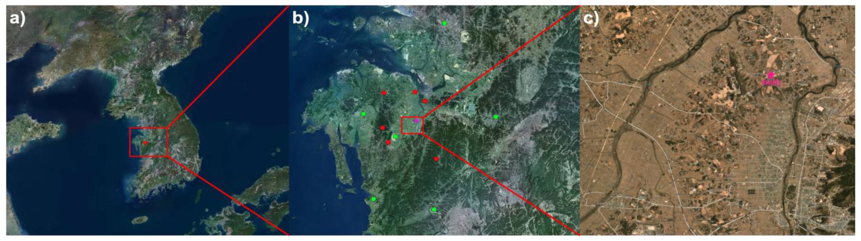
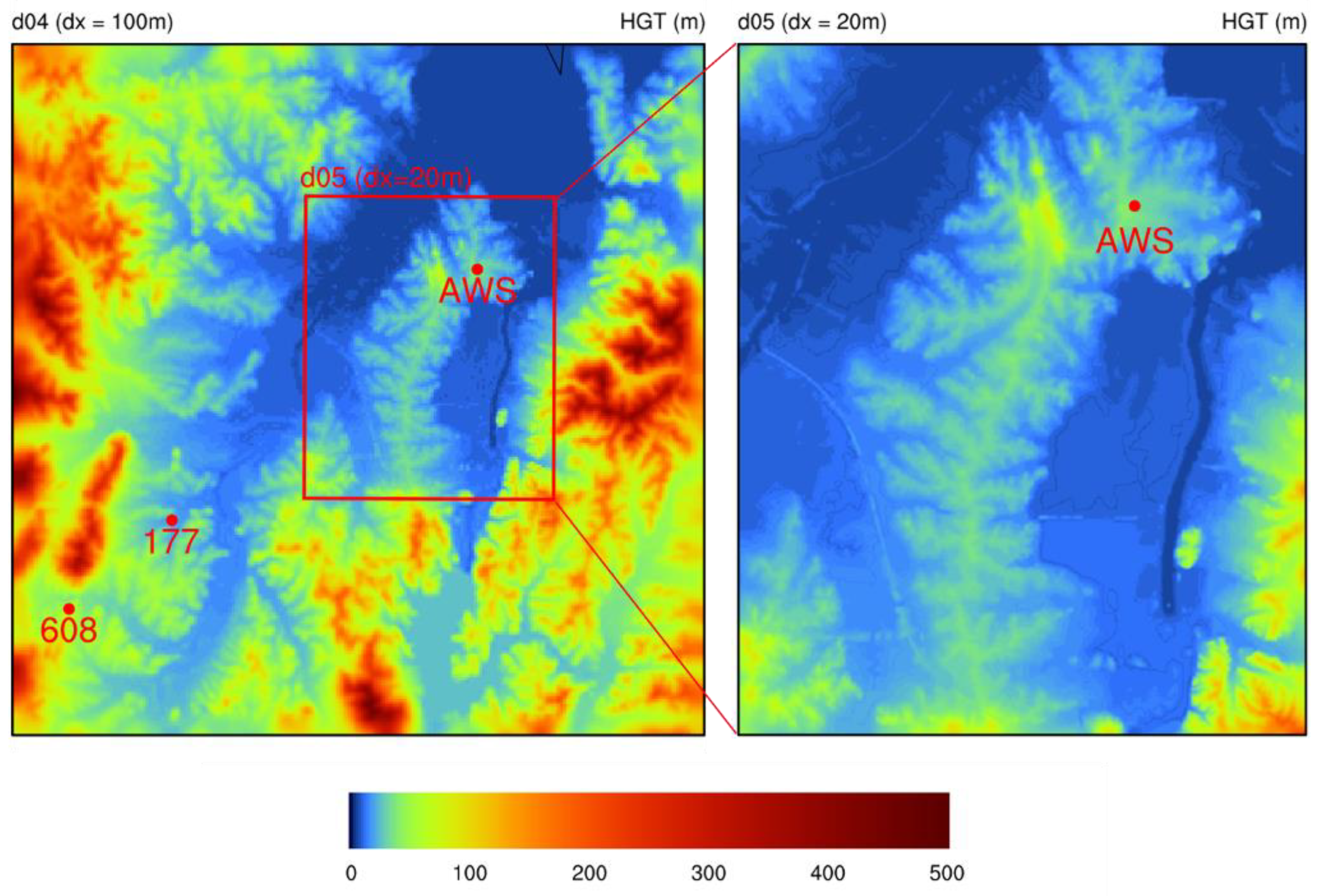
2.1. Topographical Characteristics of Study Area

The study area includes Sinam-myeon and Yesan-gun, which together represent the main apple-producing area in South Korea. It is located about 100 km south of Seoul and about 80 km northwest of Daejeon. Small-scale orchards are distributed on a wide plain, and a river is divided into two branches that flow from north to south (Figure 1).

2.2. Weather Observation Data

In the study area, two adjacent AWSs are present at the same location (Figure 2). One has been in operation since 1992 (Station number: 628, Station name: YESAN) by the Korea Meteorological Administration (KMA), and the other since 2017 (4708, SINAM) by the Rural Development Administration (RDA). The AWSs are isolated only by a fence of approximately 5 m × 8 m on a lawn constructed on one side of the parking lot in front of the main building of the Yesan Agricultural Technology Center.

Both stations observe air temperature, wind direction, wind speed, mean sea level pressure, and precipitation. The thermometers installed at the stations have a resolution of 0.1 °C and an accuracy of 0.1 °C (Site No. 628) and 0.2 °C (Site No. 4708), respectively. The anemometers at both stations have a resolution of 0.1 m/s and an accuracy of 0.5 m/s.

2.3. Climatological Analysis

Prior to the high-resolution WRF–LES simulation, the past temperature records were analyzed for the dates when low temperatures occurred at the study area. The observation data during 48 years from six neighboring Automated Synoptic Observing Systems (ASOS; Figure 1b, green markers) near YESAN (Figure 1b, pink star) and six AWS sites (Figure 1b, red marker) were used. The criteria of low temperature are set to the daily minimum temperature below 0 or −2.2 °C on the basis of the early warning system for agrometeorological hazard by the RDA [33] and the frost damage from the flowering to the full bloom on apple trees [34].

Figure 3 shows the comparison of the number of days with the daily minimum temperature below the low-temperature criterion at 13 observatories. YESAN was found to be close to the average number of low-temperature days for both 0 and −2.2 °C criteria. This indicates that the study area has very little local low-temperature specificity.

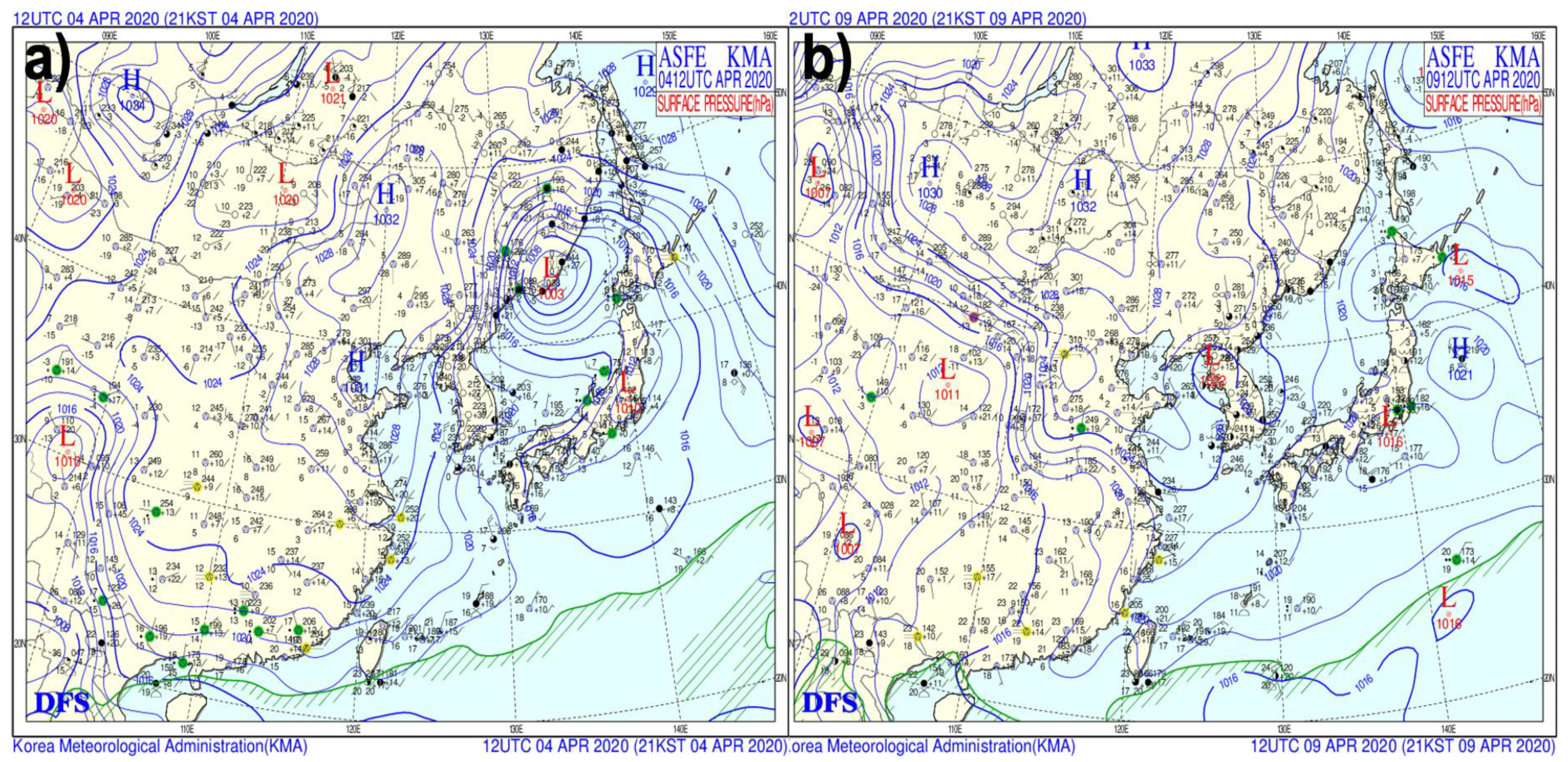
2.4. Frost Damage Cases

We investigated the days when frost or low-temperature damage happened to orchards nationwide for the recent three years (2018–2020). According to the survey by the Ministry of Agriculture, Food and Rural Affairs, the top three dates of severe frost damage to orchards are 7 April 2018 (total 5500 ha including apple tree fields of 509 ha), 4–5 April 2020 (total 4387 ha including apple tree fields of 739 ha), and 9–10 April 2020 (total 7374 ha including apple tree fields of 1936 ha). Among these cases, 4–5 April (Case 1; Figure 2) and 9–10 April 2020 (Case 2) were selected as the numerical simulation test case dates.

The case of 4–5 April 2020 was chosen because frost damage was observed at sub-zero temperatures during these days. After a low-pressure system passed through the Korean Peninsula, the expansion of the continental anticyclones and cold air flow through the upper jet were accompanied by a dramatic decrease in air temperature throughout the region (Figure 4a). Figure 5a shows that the lowest temperature in the morning in the study area was observed to be from −2 to 1 °C, a decrease of 4–6 °C compared to the previous day.

The case of 9–10 April 2020 was chosen because frost damage occurred at above-zero temperatures. The anticyclone centered in Manchuria expanded, and the entire Korean Peninsula was affected by a stable air mass (Figure 4b). The air mass was stable as the wind speed was low, and there were no low-altitude clouds. Due to this, nighttime radiative cooling occurred. Figure 5b shows the lowest temperature in the morning of 10 April 2020, when a temperature of approximately 0–3 °C was observed in the study area.

2.5. WRF–LES Model Setup

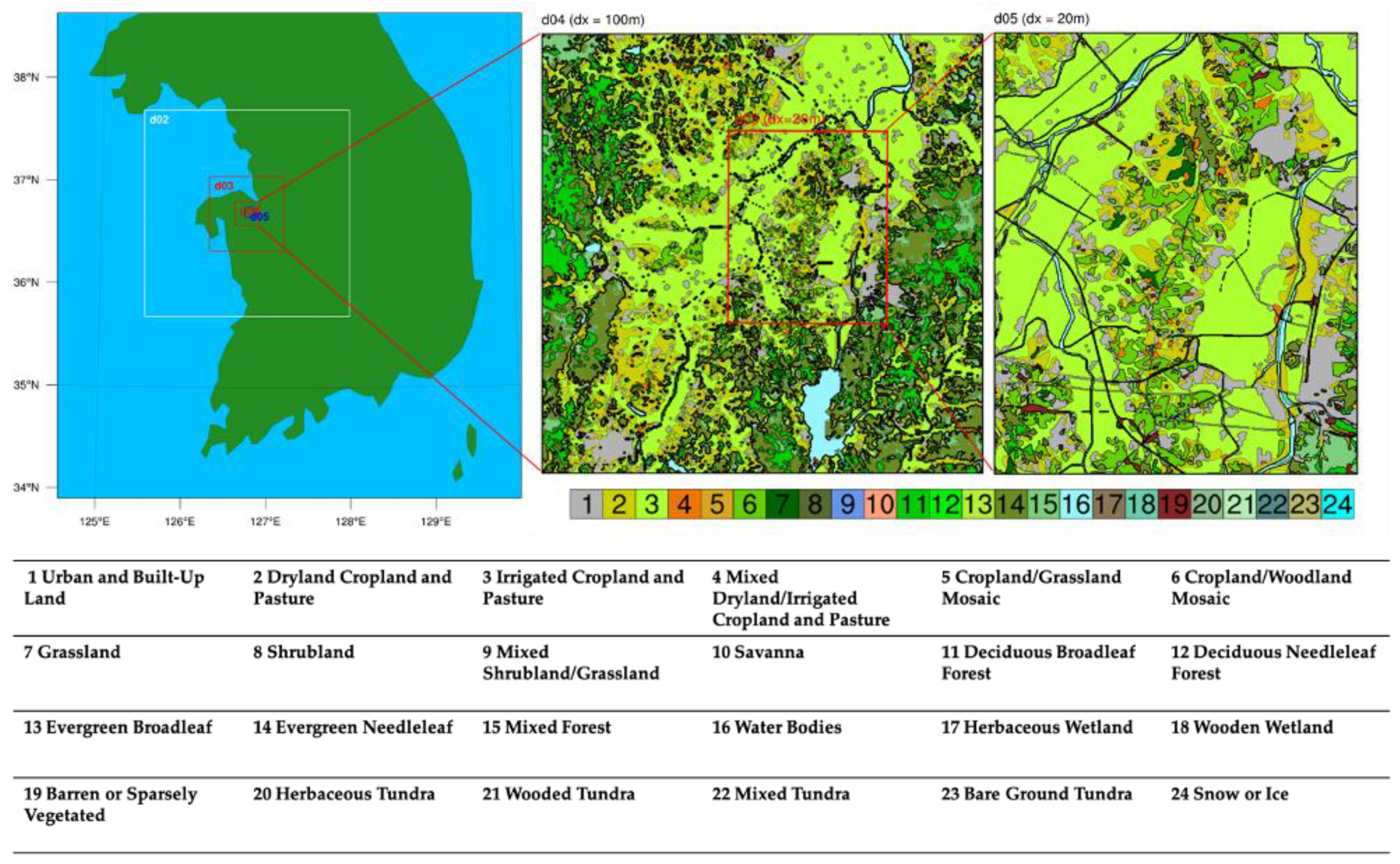
2.5.1. Domain Configuration and Physical Scheme Specification

The latest WRF version 4.1.4 was used in our simulation. FNL (final) 0.25° global tropospheric analyses and forecast data provided by the National Centers for Environmental Prediction (NCEP) were used for initial and boundary conditions. For high-resolution modeling at a spatial resolution of 20 m, five nested domains were configured. The multinested domain was applied to provide initial and boundary conditions to the high-resolution domain and to perform stable numerical calculations (Figure 6). In the innermost two domains, the LES technique was applied instead of the planetary boundary layer (PBL) scheme (

Table 1. WRF–LES specification for each domain.

Domain	PBL Scheme	dx, dy (m)	Grid Points	Time Step (s)
D01	Shin–Hong PBL	2700	187 × 196 × 81	15
D02	Shin–Hong PBL	900	247 × 250 × 81	5
D03	Shin–Hong PBL	300	271 × 271 × 81	5/3
D04	LES	100	259 × 259 × 81	5/9
D05	LES	20	461 × 561 × 81	5/54

). This enables us to simulate complex PBLs and near-surface weather where both turbulent and mesoscale motions of interest are explicitly resolved.

Table 2. Model physical parameterization settings for nested domain.

	D01	D02	D03	D04	D05
Microphysics	WDM6
Longwave radiation	RRTM scheme
Shortwave radiation	Dudhia scheme
Cumulus	Kain–Fritsch scheme		Off
PBL	Shin–Hong scheme		Off
Diffusion	Simple diffusion		Full diffusion
K option	2D deformation		3D TKE
Surface layer	Monin–Obukhov scheme

describes the model’s physical parameterization settings. WRF Double-Moment 6-class microphysics scheme [35], Rapid Radiative Transfer Model (RRTM) longwave radiation [36], Dudhia shortwave radiation [37], Monin–Obukhov surface layer scheme [38], and Kain–Fritsch cumulus parameterization [39] were applied. The Shin–Hong PBL scheme [40] was applied for the first three domains, and the LES was configured in the last two domains. Mixing in physical space, full diffusion, and 3D turbulence kinetic energy (TKE) closure K were used without the PBL scheme.

For the LES technique applied in this study [12], the eddy-viscosity of the sub-grid scale was calculated as follows:

$$K_{h,v}=C_k{l}_{h,v}\sqrt{e}$$

(1)

where e is the turbulent kinetic energy, C_k is a constant (typically 0.15 < C_k < 0.25), and l is a length scale. l_h and l_v are defined anisotropically as follows:

$$l_h=\sqrt{∆x∆y}$$

(2)

$$l_v=\{\begin{array}{c}\min \left[∆z, 0.76\frac{\sqrt{e}}{N}\right] for N^2>0\\ ∆z for N^2\le 0\end{array}$$

(3)

where N² is the Brunt–Väisälä frequency.

The TKE coefficient C_k was set to 0.15, which is the WRF default value. Previous studies have tested different coefficients [13,19], while others have attempted to improve the TKE coefficient empirically or parametrically [41,42]. However, the TKE order−1.5 model adopted in the present study did not differ evidently from the C_k values of 0.1 and 0.15 [19]. Thus, we did not conduct the sensitivity test for C_k.

A 30-arcsecond United States Geological Survey (USGS) land-use and topography dataset was used for domains 1 and 2. The spatial resolution of domains 3, 4, and 5 was higher than 30 arcseconds. Therefore, 1/3 arcsecond land-cover data provided by the Ministry of Environment of Korea and 1/3 arcsecond topography data provided by the National Geographic Information Institute were used (Figure 6).

2.5.2. Performance Measures for Model Evaluation

The WRF–LES modeling results from domain 4 (dx = 100 m) and domain 5 (dx = 20 m) were used for evaluation. Figure 7 shows the model topography and location of the AWS sites in domains 4 and 5. The comparison of AWS observation data located in the corresponding domain and the WRF–LES simulation result at the nearest grid point from the AWS site were conducted.

The mean bias (MB) and root mean square error (RMSE) were calculated from 2 m air temperature (T2, °C) and 10 m wind speed (WS, m/s) using 10 min interval WRF–LES model results and observation data. The wind speed outputs of the model are values at an altitude of 10 m from the surface. The wind data from the AWS #4708, which is located in a range of domain 5, was not applied for validation because its anemometer was above 3 m from the land surface and not at 10 m. Therefore, only AWS #628′s wind data are used for validation. If MB and RMSE are nearly 0, the model result is similar to the observed and they are calculated as follows:

$$MB=\frac{1}{n}{\displaystyle \sum }_{i=1}^n\left(x_{1i}-x_{2i}\right)$$

(4)

$$RMSE=\sqrt{\frac{{{\displaystyle \sum }}_{i=1}^n{\left(x_{1i}-x_{2i}\right)}^2}{n}}$$

(5)

3. Result and Discussion

Figure 8 illustrates the horizontal distribution of daily minimum temperature from the model-simulated data for the domain 2 (Figure 8a,b) and domain 4 (Figure 8c,d). When compared with the AWS observation data with interpolation applied (Figure 5), the WRF results appear to adequately simulate the horizontal temperature distribution in the study area.

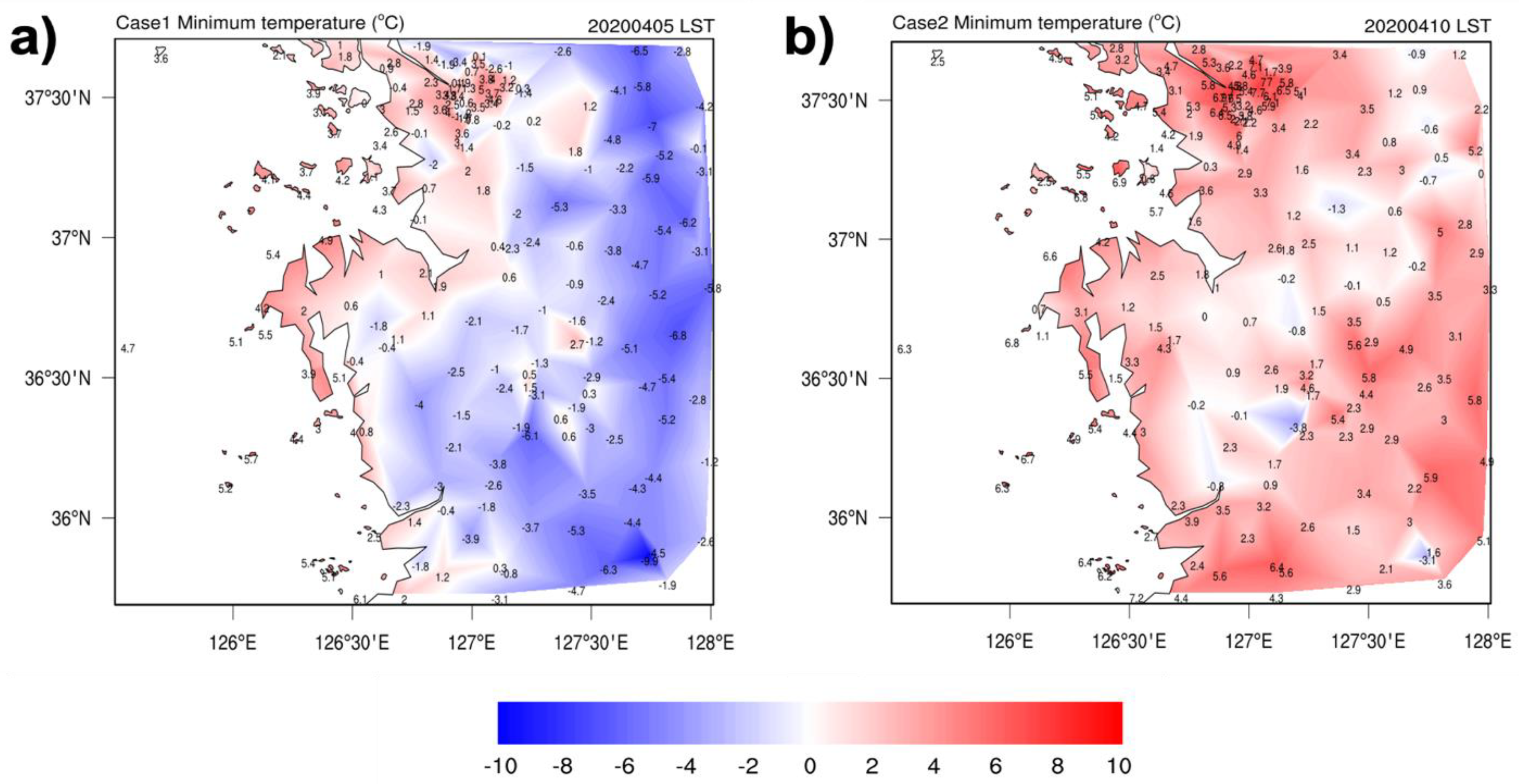
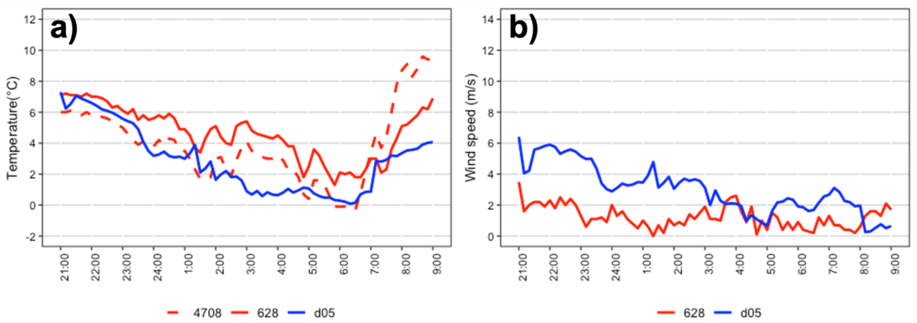
3.1. Case 1 (4–5 April 2020)

Table 3. Performance of WRF–LES simulation for Case 1.

Domain	AWS Site Number	Variable	MB	RMSE
D04	177	T2	−0.50	1.33
		WS	−0.13	1.92
	608	T2	0.50	1.31
		WS	−0.72	1.92
	628	T2	0.66	1.47
		WS	0.60	1.36
	4708	T2	1.43	4.48
D05	628	T2	−1.75	2.13
		WS	1.78	2.31
	4708	T2	−0.98	2.13

shows WRF–LES results in domains 4 and 5 for 4–5 April 2020. The MB of the temperature varied between −0.5 and −1.75 °C (average = 0.85 °C), while the RMSE varied from 1.31 to 4.48 °C (average = 2.14 °C). For wind speeds, the minimum, maximum, and average MB were −0.13, 1.78, and 0.38 m/s, respectively, while the minimum, maximum, and average RMSE were 1.36, 2.31, and 1.88 m/s, respectively.

Figure 9 shows temperature and wind speed observations from the AWSs, and WRF–LES results at the nearest grid point from the AWS site in domain 5. The temperature trend and the period in which the minimum temperature persists were similar to the observations, while the rapidly rising trend after sunrise (06:13 LST) was underestimated. The observed wind speed in Case 1 was 0–2 m/s. The WRF–LES wind simulations overestimated the observations at the beginning but became close to the observed values over time. The observed temperature showed the fluctuating behaviors. The main driver is likely the nearby technology center building located at a distance of approximately 50 m. As reported by Choi et al. [43], more systematic inspection of the meteorological observation environment of the AWS site is necessary in the future to reveal the exact influence of the surrounding anthropogenic environment on the quality of observed data.

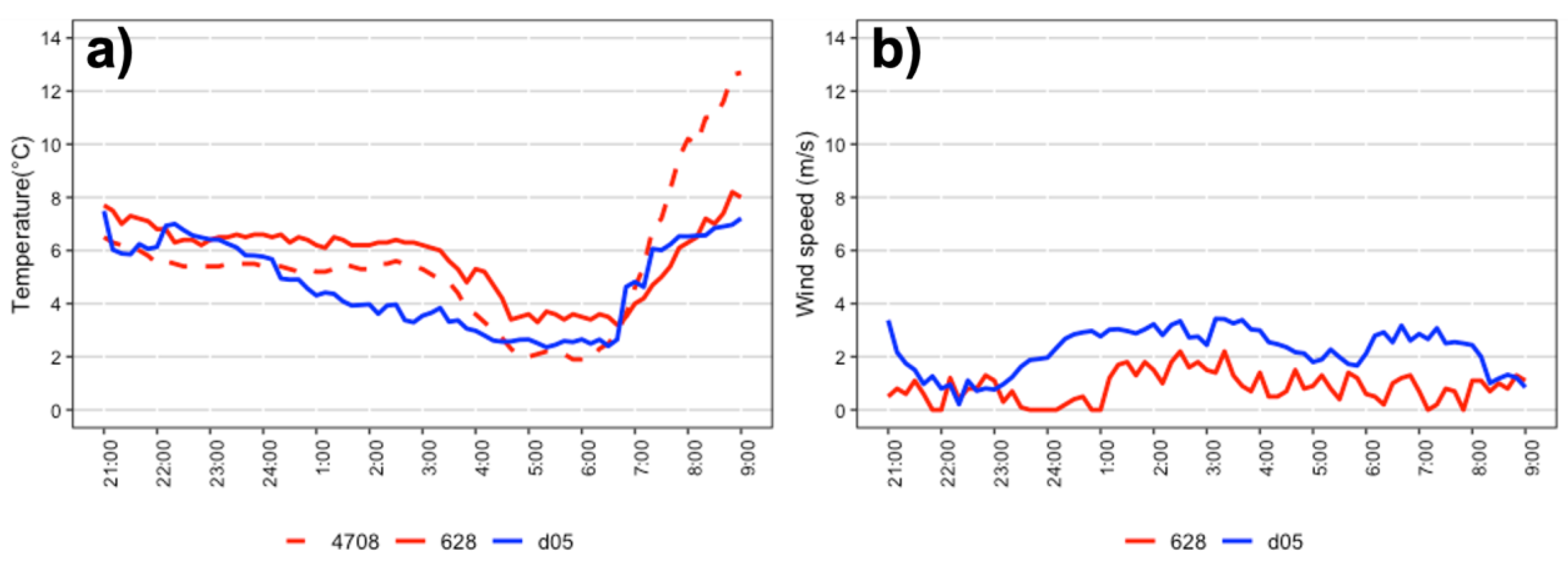
3.2. Case 2 (9–10 April 2020)

Table 4. Performance of WRF–LES simulation for Case 2.

Domain	AWS Site Number	Variable	MB	RMSE
D04	177	T2	−1.11	2.28
		WS	4.55	24.76
	608	T2	0.26	1.41
		WS	4.52	25.69
	628	T2	−2.30	6.90
		WS	2.22	7.37
	4708	T2	−1.95	9.60
D05	628	T2	−1.02	2.22
		WS	1.37	2.64
	4708	T2	−0.68	3.00

shows WRF–LES results in domain 4 and 5 on 9–10 April 2020. The MB of temperature varied from 0.26 to −2.30 °C (average = −1.13 °C), while the RMSE fluctuated between 1.41 and 9.60 °C (average = 4.23 °C). For wind speeds, MB exhibited a minimum, maximum, and average of 1.37, 4.55, and 3.16 m/s, respectively, while the RMSE showed a minimum, maximum, and average of 2.64, 25.69, and 15.11 m/s, respectively.

Figure 10 shows the AWS temperature and wind speed observations and WRF–LES results at the nearest grid point from the AWS site in domain 5. Compared to Case 1, temperature trends and the period of the lowest temperature persistence were much more similar to the observations. Nevertheless, the rapidly rising temperature changes after sunrise were still somewhat underestimated. Wind speeds showed a similar trend to observations with distributions from 0 to 2 m/s but were simulated reasonably overall.

4. Summary and Concluding Remarks

In order to predict the frost damage to field crops using the state-of-the-art WRF–LES version with high spatial resolution, the apple tree production area was selected as study area. First, the climatological analysis of long-term observation data indicated that the low temperature occurrence frequency was in a normal range when daily minimum temperature below 0 °C or below −2.2 °C was used as a criterion.

Next, five multinested domains were constructed in the WRF–LES system using domestic high-resolution domestic topography and land-cover data. The highest resolution of 20 m was applied to nighttime near-surface temperature and wind speed simulation for two recent low-temperature events that caused substantial damage to apple trees in South Korea. Combined analysis of simulations for the two cases showed that the maximum mean bias of temperature was −1.75 °C and the minimum was −0.68 °C, while the root mean square error varied between 2.13 and 3.00 °C. The high-resolution modeling application of the WRF–LES technique in the strong nighttime radiative cooling cases simulated the nocturnal temperature decrease quite well until sunrise. It is encouraging because the magnitude of model error was similar to that reported for the rural flat terrain of the Local Data Assimilation and Prediction System (LDAPS, dx = 1500 m), which is an operational forecast model of KMA [44].

Overall, the temperature simulations underestimated observations, while wind speed simulations overestimated observations, followed by a rapid rise in temperature after sunrise. In particular, the minimum temperature at dawn and its persistent duration were very reasonably reproduced by the simulations in these cases. On days with severe frost damage to orchards, the wind speed had a relatively small influence because the wind speed was very low within a stable air mass, and the temperature and duration of the minimum temperature significantly affected frost damage. Therefore, the above results demonstrate that frost damage forecast using WRF–LES is beneficial in terms of the considerable agreement with the observed patterns and its acceptable accuracy in prediction.

The WRF–LES configured in this study has become an additional component of the Land–Atmosphere Modeling Package (LAMP) of the National Center for AgroMeteorology (NCAM) [45]. It will be used to evaluate the effect of the construction of artificial structures, such as highways, buildings, airports, ports, dams, and incinerators, on the atmospheric and land environments in agricultural and forest areas with spatial resolution of tens of meters.

References

1. Hatfield, J.L.; Prueger, J.H. Temperature extremes: Effect on plant growth and development. Weather Clim. Extrem. 2015, 10, 4–10. [Google Scholar] [CrossRef] [Green Version]
2. Proebsting, E.L.; Mills, H.H. Low-temperature resistance of developing flower buds of 6 deciduous fruit species. J. Am. Soc. Hortic. Sci. 1978, 103, 192–198. [Google Scholar]
3. Rodrigo, J. Spring frosts in deciduous fruit trees—Morphological damage and flower hardiness. Sci. Hortic. 2000, 85, 155–173. [Google Scholar] [CrossRef]
4. Snyder, R.; Paw, U.K.; Thompson, J. Passive Frost Protection of Trees and Vines; University of California: Los Angeles, CA, USA, 1987; Available online: https://anrcatalog.ucanr.edu/pdf/21429e.pdf (accessed on 19 November 2021).
5. Snyder, R.L.; Melo-Abreu, J.D. Frost Protection: Fundamentals, Practice and Economics; FAO: Rome, Italy, 2005; Volume 1, pp. 1–240. [Google Scholar]
6. Lindkvist, L.; Gustavsson, T.; Bogren, J. A frost assessment method for mountainous areas. Agric. For. Meteorol. 2000, 102, 51–67. [Google Scholar] [CrossRef]
7. Mahrt, L.; Sun, J.L.; Oncley, S.P.; Horst, T.W. Transient Cold Air Drainage down a Shallow Valley. J. Atmos. Sci. 2014, 71, 2534–2544. [Google Scholar] [CrossRef]
8. Chung, U.; Seo, H.H.; Hwang, K.H.; Hwang, B.S.; Choi, J.; Lee, J.T.; Yun, J.I. Minimum temperature mapping over complex terrain by estimating cold air accumulation potential. Agric. For. Meteorol. 2006, 137, 15–24. [Google Scholar] [CrossRef]
9. Holden, Z.A.; Abatzoglou, J.T.; Luce, C.H.; Baggett, L.S. Empirical downscaling of daily minimum air temperature at very fine resolutions in complex terrain. Agric. For. Meteorol. 2011, 151, 1066–1073. [Google Scholar] [CrossRef]
10. Ashcroft, M.B.; Gollan, J.R. Fine-resolution (25 m) topoclimatic grids of near-surface (5 cm) extreme temperatures and humidities across various habitats in a large (200 × 300 km) and diverse region. Int. J. Climatol. 2012, 32, 2134–2148. [Google Scholar] [CrossRef] [Green Version]
11. Gobbett, D.L.; Nidumolu, U.; Crimp, S. Modelling frost generates insights for managing risk of minimum temperature extremes. Weather Clim. Extrem. 2020, 27, 9. [Google Scholar] [CrossRef]
12. Skamarock, W.C.; Klemp, J.B.; Dudhia, J.; Gill, D.O.; Liu, Z.; Berner, J.; Wang, W.; Powers, J.G.; Duda, M.G.; Barker, D.; et al. A Description of the Advanced Research WRF Model Version 4; National Center for Atmospheric Research: Boulder, CO, USA, 2019. [CrossRef]
13. Moeng, C.H.; Dudhia, J.; Klemp, J.; Sullivan, P. Examining two-way grid nesting for large eddy simulation of the PBL using the WRF model. Mon. Weather Rev. 2007, 135, 2295–2311. [Google Scholar] [CrossRef]
14. Moeng, C.H. A Large-eddy-simulation model for the study of planetary boundary-layer turbulence. J. Atmos. Sci. 1984, 41, 2052–2062. [Google Scholar] [CrossRef]
15. Parodi, A.; Tanelli, S. Influence of turbulence parameterizations on high-resolution numerical modeling of tropical convection observed during the TC4 field campaign. J. Geophys. Res. Atmos. 2010, 115. [Google Scholar] [CrossRef]
16. Gibbs, J.A.; Fedorovich, E. Comparison of Convective Boundary Layer Velocity Spectra Retrieved from Large-Eddy-Simulation and Weather Research and Forecasting Model Data. J. Appl. Meteorol. Climatol. 2014, 53, 377–394. [Google Scholar] [CrossRef]
17. Munoz-Esparza, D.; Kosovic, B.; Garcia-Sanchez, C.; van Beeck, J. Nesting Turbulence in an Offshore Convective Boundary Layer Using Large-Eddy Simulations. Bound. Layer Meteorol. 2014, 151, 453–478. [Google Scholar] [CrossRef]
18. Heath, N.K.; Fuelberg, H.E.; Tanelli, S.; Turk, F.J.; Lawson, R.P.; Woods, S.; Freeman, S. WRF nested large-eddy simulations of deep convection during SEAC(4)RS. J. Geophys. Res. Atmos. 2017, 122, 3953–3974. [Google Scholar] [CrossRef]
19. Simon, J.S.; Zhou, B.W.; Mirocha, J.D.; Chow, F.K. Explicit Filtering and Reconstruction to Reduce Grid Dependence in Convective Boundary Layer Simulations Using WRF-LES. Mon. Weather Rev. 2019, 147, 1805–1821. [Google Scholar] [CrossRef]
20. Zhong, J.; Nikolova, I.; Cai, X.; MacKenzie, A.R.; Alam, M.S.; Xu, R.; Singh, A.; Harrison, R.M. Traffic-induced multicomponent ultrafine particle microphysics in the WRF v3.6.1 large eddy simulation model: General behaviour from idealised scenarios at the neighbourhood-scale. Atmos. Environ. 2020, 223. [Google Scholar] [CrossRef]
21. Cece, R.; Bernard, D.; Brioude, J.; Zahibo, N. Microscale anthropogenic pollution modelling in a small tropical island during weak trade winds: Lagrangian particle dispersion simulations using real nested LES meteorological fields. Atmos. Environ. 2016, 139, 98–112. [Google Scholar] [CrossRef]
22. Liu, Y.J.; Liu, Y.B.; Munoz-Esparza, D.; Hu, F.; Yan, C.; Miao, S.G. Simulation of Flow Fields in Complex Terrain with WRF-LES: Sensitivity Assessment of Different PBL Treatments. J. Appl. Meteorol. Climatol. 2020, 59, 1481–1501. [Google Scholar] [CrossRef]
23. Udina, M.; Montornes, A.; Casso, P.; Kosovic, B.; Bech, J. WRF-LES Simulation of the Boundary Layer Turbulent Processes during the BLLAST Campaign. Atmosphere 2020, 11, 1149. [Google Scholar] [CrossRef]
24. Huang, Y.J.; Liu, Y.B.; Liu, Y.W.; Li, H.Y.; Knievel, J.C. Mechanisms for a Record-Breaking Rainfall in the Coastal Metropolitan City of Guangzhou, China: Observation Analysis and Nested Very Large Eddy Simulation With the WRF Model. J. Geophys. Res. Atmos. 2019, 124, 1370–1391. [Google Scholar] [CrossRef]
25. Cui, C.X.; Bao, Y.X.; Yuan, C.S.; Li, Z.H.; Zong, C. Comparison of the performances between the WRF and WRF-LES models in radiation fog—A case study. Atmos. Res. 2019, 226, 76–86. [Google Scholar] [CrossRef]
26. Talbot, C.; Bou-Zeid, E.; Smith, J. Nested Mesoscale Large-Eddy Simulations with WRF: Performance in Real Test Cases. J. Hydrometeorol. 2012, 13, 1421–1441. [Google Scholar] [CrossRef]
27. Cuchiara, G.C.; Rappengluck, B. Performance analysis of WRF and LES in describing the evolution and structure of the planetary boundary layer. Environ. Fluid Mech. 2018, 18, 1257–1273. [Google Scholar] [CrossRef]
28. Simon, J.S.; Bragg, A.D.; Dirmeyer, P.A.; Chaney, N.W. Semi-Coupling of a Field-Scale Resolving Land-Surface Model and WRF-LES to Investigate the Influence of Land-Surface Heterogeneity on Cloud Development. J. Adv. Model. Earth Syst. 2021, 13, 24. [Google Scholar] [CrossRef]
29. Zhu, P. A multiple scale modeling system for coastal hurricane wind damage mitigation. Nat. Hazards 2008, 47, 577–591. [Google Scholar] [CrossRef]
30. Zhu, P. Simulation and parameterization of the turbulent transport in the hurricane boundary layer by large eddies. J. Geophys. Res. Atmos. 2008, 113, 16. [Google Scholar] [CrossRef]
31. Munoz-Esparza, D.; Lundquist, J.K.; Sauer, J.A.; Kosovic, B.; Linn, R.R. Coupled mesoscale-LES modeling of a diurnal cycle during the CWEX-13 field campaign: From weather to boundary-layer eddies. J. Adv. Model. Earth Syst. 2017, 9, 1572–1594. [Google Scholar] [CrossRef]
32. Bauer, H.S.; Muppa, S.K.; Wulfmeyer, V.; Behrendt, A.; Warrach-Sagi, K.; Spath, F. Multi-nested WRF simulations for studying planetary boundary layer processes on the turbulence-permitting scale in a realistic mesoscale environment. Tellus Ser. A-Dyn. Meteorol. Oceanol. 2020, 72, 28. [Google Scholar] [CrossRef]
33. Early Warning System for Agrometeorological Hazard. Available online: http://www.agmet.kr (accessed on 19 November 2021).
34. Kim, J.-H.; Kim, D.-j.; Kim, S.-o.; Yun, E.-j.; Ju, O.; Park, J.S.; Shin, Y.S. Estimation of freeze damage risk according to developmental stage of fruit flower buds in spring. Korean J. Agric. For. Meteorol. 2019, 21, 55–64. [Google Scholar] [CrossRef]
35. Lim, K.S.S.; Hong, S.Y. Development of an Effective Double-Moment Cloud Microphysics Scheme with Prognostic Cloud Condensation Nuclei (CCN) for Weather and Climate Models. Mon. Weather Rev. 2010, 138, 1587–1612. [Google Scholar] [CrossRef] [Green Version]
36. Mlawer, E.J.; Taubman, S.J.; Brown, P.D.; Iacono, M.J.; Clough, S.A. Radiative transfer for inhomogeneous atmospheres: RRTM, a validated correlated-k model for the longwave. J. Geophys. Res. Atmos. 1997, 102, 16663–16682. [Google Scholar] [CrossRef] [Green Version]
37. Dudhia, J. Numerical study of convection observed during the winter monsoon experiment using a mesoscale two-dimensional model. J. Atmos. Sci. 1989, 46, 3077–3107. [Google Scholar] [CrossRef]
38. Monin, A.S.; Obukhov, A.M. Basic laws of turbulent mixing in the surface layer of the atmosphere. Contrib. Geophys. Inst. Acad. Sci. USSR 1954, 151, e187. [Google Scholar]
39. Kain, J.S. The Kain-Fritsch convective parameterization: An update. J. Appl. Meteorol. 2004, 43, 170–181. [Google Scholar] [CrossRef] [Green Version]
40. Shin, H.H.; Hong, S.Y. Representation of the Subgrid-Scale Turbulent Transport in Convective Boundary Layers at Gray-Zone Resolutions. Mon. Weather Rev. 2015, 143, 250–271. [Google Scholar] [CrossRef]
41. Kovadlo, P.G.; Lukin, V.P.; Shikhovtsev, A.Y. Development of the Model of Turbulent Atmosphere at the Large Solar Vacuum Telescope Site as Applied to Image Adaptation. Atmos. Ocean. Opt. 2019, 32, 202–206. [Google Scholar] [CrossRef]
42. Archer, C.L.; Wu, S.C.; Ma, Y.L.; Jimenez, P.A. Two Corrections for Turbulent Kinetic Energy Generated by Wind Farms in the WRF Model. Mon. Weather Rev. 2020, 148, 4823–4835. [Google Scholar] [CrossRef]
43. Choi, S.-W.; Lee, S.-J.; Kim, J.; Lee, B.-L.; Kim, K.-R.; Choi, B.-C. Agrometeorological observation environment and periodic report of Korea Meteorological Administration: Current status and suggestions. Korean J. Agric. For. Meteorol. 2015, 17, 144–155. [Google Scholar] [CrossRef] [Green Version]
44. Kim, D.J.; Kang, G.; Kim, D.; Kim, J.J. Characteristics of LDAPS-Predicted Surface Wind Speed and Temperature at Automated Weather Stations with Different Surrounding Land Cover and Topography in Korea. Atmosphere 2020, 11, 1224. [Google Scholar] [CrossRef]
45. Lee, S.-J.; Song, J.; Kim, Y.-J. The NCAM Land-Atmosphere Modeling Package (LAMP) Version 1: Implementation and Evaluation. Korean J. Agric. For. Meteorol. 2016, 18. [Google Scholar] [CrossRef] [Green Version]
Figure 1. (a) Satellite image of Korea provided by KakaoMap. (b) Weather station sites of the Korea Meteorological Administration (red circles: automatic weather station, green circles: Automated Synoptic Observing System, pink star: Yesan weather station). (c) Satellite image of study area in April 2020, provided by Planet Lab, and location of weather station (pink star).
Atmosphere 12 01562 g001
Figure 2. Left panel is two automatic weather stations of Korea Meteorological Administration (right tower) and Rural Development Administration (left tower) at the study area shown in Figure 1c. Right panels show crop damages due to sudden low temperature or frost (1: The petals of pear blossoms and the top of the ovary turned black; 2: Peach flowers that turned dark red; 3: The icicles on the pear tree and the frozen spray water; 4: The apple, which is in the state of a bud, turned yellow in the temperature that fell below zero (Source: © Nongmin News Corp. with photographs by Gyo-Hyun Chu).
Atmosphere 12 01562 g002
Figure 3. Number of days with the minimum temperature (Tmin) (a) below 0 °C and (b) below −2.2 °C noted at each observation station (x, ASOS; blue filled circle, AWS; and green filled circle, YESAN). Red lines represent the average of the 13 stations for each month and black bars show standard variation of each station.
Atmosphere 12 01562 g003
Figure 4. The 12 UTC (21 LST) surface weather chart for (a) 4 April 2020 and (b) 9 April 2020.
Atmosphere 12 01562 g004
Figure 5. Daily minimum temperature (°C) on (a) 5 April 2020 (Case 1) and (b) 10 April 2020 over the study domain (Case 2).
Atmosphere 12 01562 g005
Figure 6. Domain configuration of WRF–LES and implementation of high-resolution domestic land-cover data.
Atmosphere 12 01562 g006
Figure 7. High-resolution terrain height (m) data and AWS sites at domain 4 and domain 5.
Atmosphere 12 01562 g007
Figure 8. WRF-simulated result of daily minimum air temperature (°C) for domain 2 (a,b) and WRF–LES-simulated results for domain 4 (c,d).
Atmosphere 12 01562 g008
Figure 9. Comparison of time series of observed data at AWS (#4708 and #628) and WRF–LES simulation in domain 5 for Case 1. (a) The 2 m air temperature (°C) and (b) wind speed (m/s).
Atmosphere 12 01562 g009
Figure 10. Comparison of time series of observed data at AWS (#4708 and #628) and WRF–LES simulation in domain 5 for Case 2. (a) The 2-m air temperature (°C) and (b) wind speed (m/s).
Atmosphere 12 01562 g010