Article

Observation-Based Summer O3 Control Effect Evaluation: A Case Study in Chengdu, a Megacity in Sichuan Basin, China

1
College of Architecture and Environment, Sichuan University, Chengdu 610065, China
2
Chengdu Academy of Environmental Sciences, Chengdu 610065, China
*
Authors to whom correspondence should be addressed.
Atmosphere 2020, 11(12), 1278; https://doi.org/10.3390/atmos11121278
Submission received: 9 November 2020 / Revised: 23 November 2020 / Accepted: 24 November 2020 / Published: 26 November 2020
(This article belongs to the Special Issue Air Quality Management)

Abstract

:
Ground-level ozone (O3), which is mainly from the photochemical reactions of NOx and volatile organic compounds (VOCs), has become a crucial pollutant obstructing air quality improvement in China. Understanding the composition, temporal variability and source apportionment of VOCs is necessary for determining effective control measures to minimize VOCs and their related photochemical pollution. To provide a comprehensive analysis of VOC sources and their contributions to ozone formation in the city of Chengdu—a megacity with the highest rates of industrial and economic development in southwest China—we conducted a one-month monitoring project at three urban sites (Shuangliu, Xindu, Junpingjie; SL, XD and JPJ, respectively) along the main north–south meteorological transport channel before and during the implemented control measures. Alkanes were the dominant group at each site, contributing to around 50% of the observed total VOCs, followed by oxygen-containing VOCs (OVOCs), aromatics, halohydrocarbons and alkenes. During the control period, the mixing ratios of most measured VOC species decreased, and O3 concentrations were down by at least 20%. VOC species experiencing the most effect from control were aromatics and OVOCs, which had higher O3 formation reactivity. This indicated that the control policies had significant influence on reductions of reactive VOC species. We also identified VOC sources at SL and XD using positive matrix factorization (PMF) and assessed their contributions to photochemical O3 formation by calculating the O3 formation potential (OFP) based on mass concentrations and maximum incremental reactivity of related VOCs. Five dominant VOC sources were identified, with the highest contributions from vehicular exhaust and fuel evaporation before control, followed by solvent utilization, biogenic background and secondary formation, and industrial emissions. Contribution from vehicular exhaust was reduced the most at SL, while at XD, secondary formation VOCs decreased significantly. VOCs from vehicular and industrial emissions and solvent utilization were found to be the dominant precursors for OFPs, particularly the species of xylenes, toluene and propene. Our results therefore suggest that priority should be given to the alleviation of photochemical pollutants for effective control of O3 formation in Chengdu. The findings from this work have important implications for formulating effective emission control policies in Chengdu.

1. Introduction

Ozone, as a main product from photochemical reactions, is now a widespread pollution problem in many of the world’s population centers, especially in China [1]. Therefore, considerable attention has been given not only to identifying and quantifying chemical processes leading to the generation of O3 and other secondary photochemical pollutants, but also to putting forward their control countermeasures. Regional ozone pollution events occur frequently over China [2,3]. Thus, it is urgent to gain in-depth knowledge about the key precursors of ozone formation and evolution, in order to adopt effective measures to improve air quality. Sichuan Basin in southwest China has complex terrain, special meteorological conditions, and a fast urbanization rate [4,5]. Chengdu, located on the western edge of Sichuan Basin, is the capital of Sichuan province and a megacity with high anthropogenic emission; the city experiences stagnant meteorological conditions frequently. Chengdu has recorded high levels of PM2.5 and O3 pollution [6,7,8].
The severity of O3 pollution has increased in Chengdu and has triggered widespread concern towards air quality improvement. In the summer of 2016 (July and August), the maximum 8 h average O3 concentration reached 322 μg/m3, and ozone alone caused 27 heavy-polluted days in Chengdu. There have been some preliminary investigations to analyze ozone pollution and its related precursors (NOx and volatile organic compounds (VOCs)) [9,10]. The temporal and spatial distribution of VOCs in Chengdu has been studied, revealing the relationship between emission source and contamination potential, and contributing to better understanding of the characteristics of VOCs and the major pollution sources [11]. From previous studies based on O3-NOx-VOCs sensitivity analysis, O3 generation was generally determined by VOCs in most urban areas of Chengdu, and anthropogenic VOC emissions might be a critical factor in O3 pollution formation in certain locations [12].
To mitigate ozone pollution in Chengdu, the Chengdu Leading Group Office of Air Pollution Prevention and Control launched a specific campaign on O3 pollution and set strict plans to reduce emissions of relevant air pollutants in the whole city from August 7 to September 7, 2017. The target sources included vehicles, paint and solvent use, iron and steel factories, chemical factories, and power plants. During the control period, about 20,000 heavy-polluting vehicles were weeded out; 542 coal-fired boilers were replaced by electricity or natural gas boilers; a total of 14,148 poorly managed polluting enterprises were banned or asked to improve; and off-peak production measures were fully implemented for key enterprises. In the city, ~75 enterprises that emitted key volatile organic compounds were required to cut output by ~50%, and ~42 enterprises that emitted key nitrogen oxides were required to cut output by ~30%. Strict control measures resulted in emission changes evident regionally that summer.
In the current investigation, we focused on understanding the variability of O3 characteristics and its precursors due to the implementation of control measures in Chengdu, based on a high-resolution observational campaign conducted simultaneously at three surveillance sites. The aim was to assess the effect of mitigation strategies on emission variability and the subsequent response from O3 concentration. Results from the current study can contribute to better understanding of the reasons for ozone pollution and its prevention and control in Sichuan Basin.

2. Methodology

2.1. Field Measurement

In Chengdu, a strict control of atmospheric pollution act was performed for one month between 7 August 2017 and 7 September 2017. To assess the control effect on O3 formation in Chengdu, field measurements were conducted at three atmospheric monitoring sites, Junpingjie site (JPJ, 104.05° N, 30.66° E), Xindu site (XD, 104.16° N, 30.79° E) and Shuangliu site (SL, 103.93° N, 30.58° E) from July 31 to August 31, 2017. JPJ is located in downtown Chengdu, an area with mixed zones of traffic and commercial and residential infrastructure. XD is north-east of downtown, which is an area upwind of the city center and the key industry in this region is logistical transportation. SL is located downwind of the city center, and is an industrial zone. The exact location of each site is given in Figure 1.
Hourly measurements of trace gases (including O3, NO2, CO, SO2) were monitored and maintained by the Chengdu Environmental Monitoring Center. The instruments used for the measurement of gaseous species, O3, NO2, CO and SO2 were Thermo Scientific, Model 49i, Model 43i, Model 48i and Model 42i, respectively. Meteorological data (i.e., temperature, relative humidity, etc.) were derived from national monitoring stations. VOC species were measured by an automated online gas chromatography–flame ionization detector/mass spectrometric detector (GC-FID/MS) system (Agilent 7890B-FID-5977A) at XD and SL, by which hourly concentrations of 99 VOC species, including 29 alkanes, 11 alkenes, 16 aromatics, 13 oxygenated VOCs, 28 halohydrocarbons, acetylene, and acetonitrile were obtained. At JPJ, only non-methane hydrocarbons (55 VOC species, including 28 alkanes, 10 alkenes, 16 aromatics and acetylene) were continuously detected using a gas chromatograph with a flame ionization detector (FID) and a dual photoionization detector (PID) (Synspec GC955-611/811). Detailed descriptions of these two instruments are provided elsewhere [13,14]. The instruments were calibrated using the VOC standards. The detection limits and the precisions of measured VOCs are listed in Table S1 of the Supplementary Materials.

2.2. VOC Reactivity and Contribution to O3 Formation

The level of VOC reactivity and sources are key factors for policy makers to consider when aiming to control local ozone contamination. There are different methods used to estimate O3 formation from VOCs [15,16,17,18]. Among them, the simple calculation of ozone formation potentials (OFPs) with maximum incremental reactivity (MIR) values of different VOC species has been widely applied in other studies [2,8,19,20,21,22,23]. In this work, the OFP values were calculated based on the observed mixing ratio of each VOC species [22,23]. The MIR values were adopted to estimate ozone formation potential of different VOC species. The following Equation (1) is used to derive the OFP values:
OFPx = [VOC]x × MIRx
where OFPx and [VOC]x are the ozone formation potential and the concentration of VOC species x, respectively, with units of μg/m3; MIR values were adopted according to Carter’s work [24].

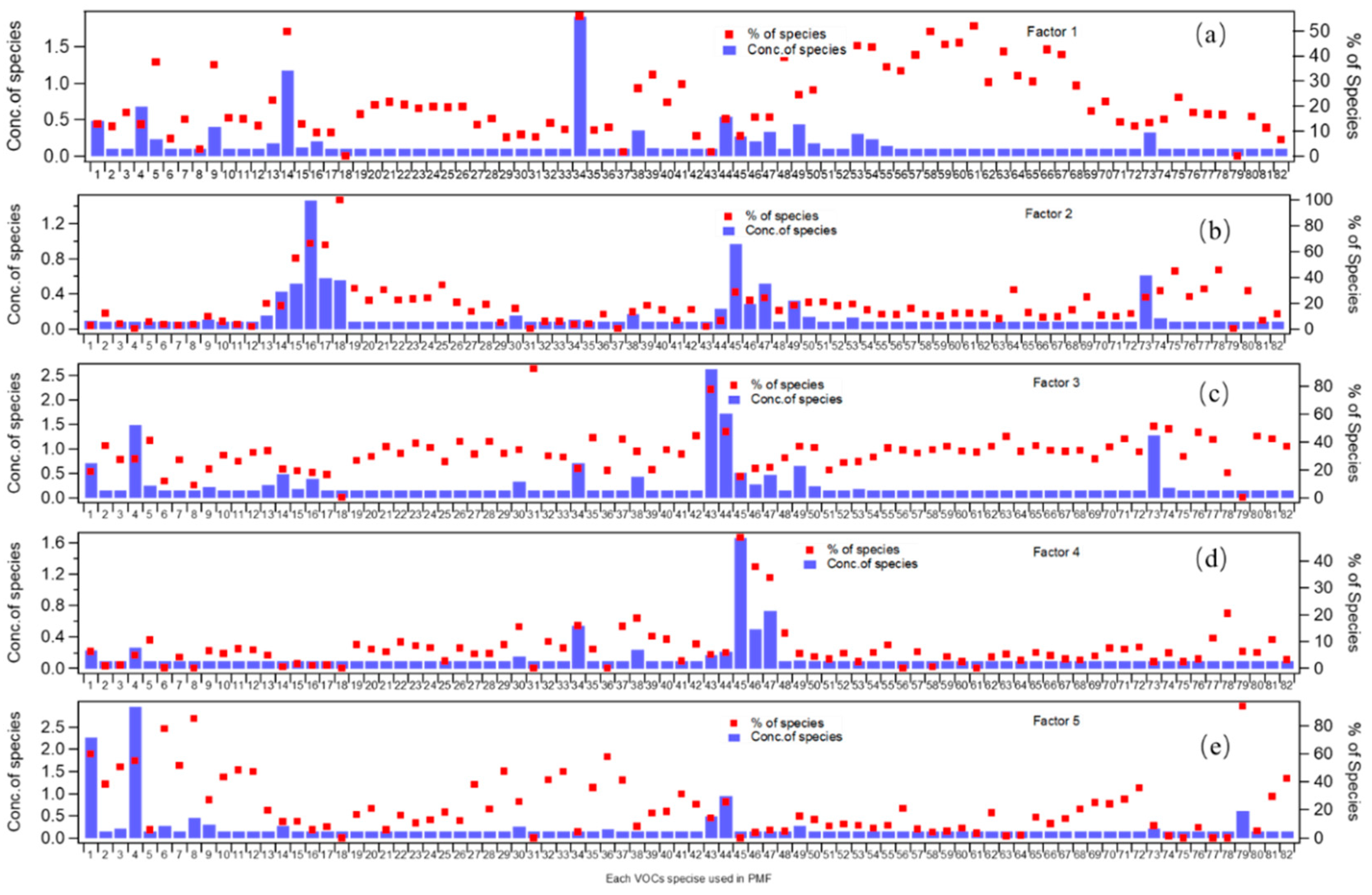
2.3. Source Apportionment

The sources of VOCs are important references for formulating and implementing effective control measures. Generally, the ratios between specific VOCs and receptor models, such as positive matrix factorization (PMF), principal component analysis-absolute principal component score (PCA-APCS) and chemical mass balance (CMB), are tools commonly used for source identification and/or apportionment. In this work, PMF model 5.0 was used to calculate the contribution of different emission sources. The principle and details of this model have been described in User Guide (U.S. EPA, 2014) and previous studies [22,25]. Briefly, the PMF model decomposes the receptor matrix (X) into the contribution matrix (G) and profile matrix (F), and then determines the main source and its contribution by the least square method [26]. In this work, we utilized VOC species measured from different sites and time periods to reflect the emission characteristics before and during the implementation of control measures. The mixing ratio of each measured VOC was used as the concentration value of each parameters, the uncertainty of each concentration was obtained from the uncertainty of GC-FID/MS analysis.
A large number of samples and strict quality control of the VOC measurements are the foundations of reasonable source apportionment. The rule of species selection included: (1) The selected species should have a relatively high concentration [27]; (2) Species with strong chemical reactivity were not involved in the calculation [28,29]; (3) The species selected to participate in the calculation should be of obvious fingerprint significance [30], (4) VOC species which poorly fitted to the PMF model were excluded. In our work, we calculated PMF solutions with 4–7 factors. The stability and uncertainty of the computed solutions were estimated by both a displacement method and a bootstrap method provided by PMF 5.0.

3. Results and Discussion

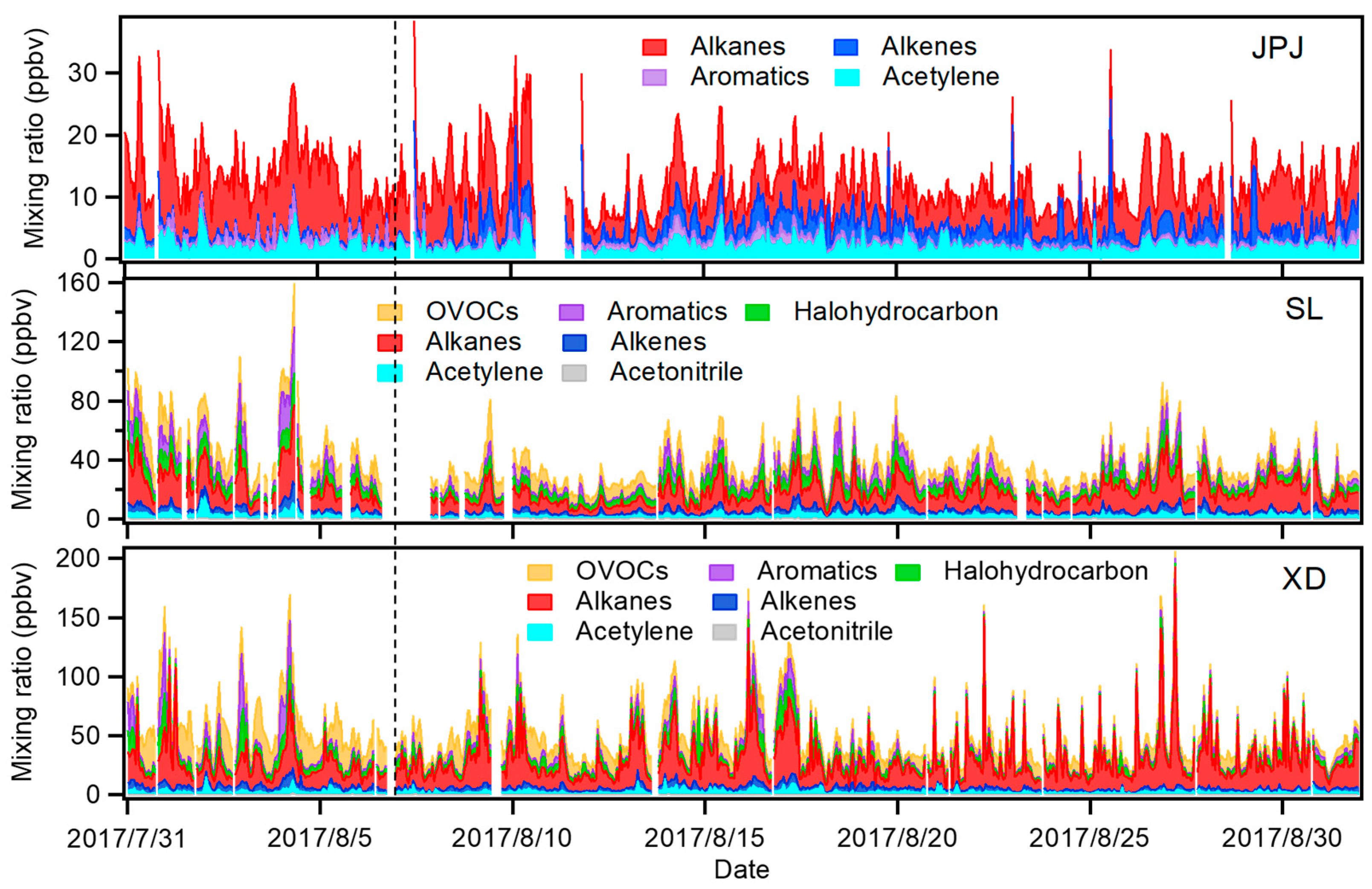
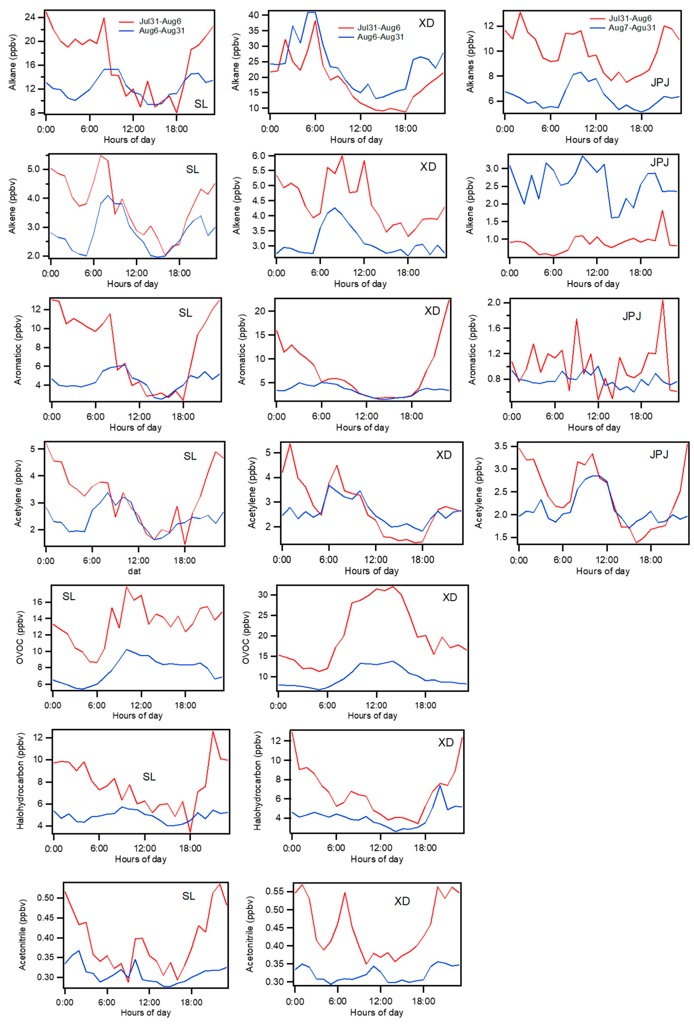
3.1. Spatial and Temporal Distribution of Ambient Air Pollutants before and during the Control Campaign

The temporal concentrations of O3, NO2, and CO at the three sites are displayed as time-series diagrams in Figure 2. Meteorological conditions such as temperature, relative humidity (RH), wind direction and wind speed are shown in Figures S1 and S2. In general, the O3 concentrations showed similar patterns at three study sites, indicating they all are subjected to similar meteorology. Before the control period, there were four out of seven days with ozone concentrations exceeding the Chinese National Air Quality Standard Grade II (Maximum 8 h concentrations >160 μg/m3), while during the control period, the ozone pollution episodes were significantly reduced (five out of twenty-five days).
Figure 3 shows the mean diurnal profiles of O3 NO2, CO concentrations at different sites before and during control periods. The maximum diurnal O3 concentrations appeared at 14:00–16:00 every day, when NO2 and CO concentrations reached their lowest values, reflecting a distinct periodic variation between precursors and their secondary pollutants. The averaged concentrations of O3, NO2 and CO before and during the control period at each site are listed in Table 1. At all study sites, O3 concentrations were down by at least 20% during the control period. However, the O3 concentration during 0:00–05:00 seems to be more during the control period at SL site. This might be due to the decrease in NO emissions during the control period, resulting in a reduction in NO titration which caused consumption of O3. In the evening, there was almost no photochemical reaction to produce O3, so less consumption could cause more accumulation of O3 in the troposphere. NO2 concentrations declined by 24.00% and 25.12% at JPJ and SL, respectively. In comparison, there was a reduction of only 11.34% at XD, probably due to the characteristics of local businesses. CO concentrations were also lower by more than 13% at all the sites, implying that controlling the amount of vehicles (cleaning up heavy-polluted vehicles) and fuel reduction (replacing coal with electricity or natural gas) played a key role in mitigating NO2 and CO concentrations.
The daily averaged ambient temperature during the measurement period changed by around 3 ℃ (Figure S1, Table S2 of the Supplementary Materials), which might reflect that solar radiation had certain influences on the formation of O3 and biogenic VOC (BVOC) emission, but likely little influence on the anthropogenic emissions. The RH varied greatly from day to night, although the mean RH remained stable (~80%) during the study period. The wind speed and direction data are provided in Figure S2 of the Supplementary Materials, which show that the wind speed during the entire period was mainly less than 2 m/s, and the dominant wind direction was typically north and northwest. The similar wind direction made it possible to compare the concentrations before and during control periods, and the meteorological conditions likely had little impact on the ambient VOC concentrations.
Time series of VOC concentrations at the three sites are displayed in Figure 4. Ambient VOC group mixing ratios and chemical compositions at each site are also summarized in Table 1. Before the control period, the mixing ratios of total VOCs averaged 14.4 ppbv, 52.8 ppbv, and 60.6 ppbv at JPJ, SL, and XD, respectively. During the control period, they were reduced to 11.8 ppbv, 34.9 ppbv, and 47.0 ppbv, respectively.
Alkanes were the most abundant VOC group both before and during the control period at each site (except for XD before the control period), comprising 62%, 33% and 40% of total VOC measured, respectively. In addition, oxygen-containing volatile organic compounds (OVOCs), which came from both primary emissions and secondary generations, were also abundant. A high mixing ratio of acetaldehyde (~10 ppbv) observed at XD before control suggested that dramatic photochemical reactions existed due to these ozone precursors. Although lower, the contribution of alkenes increased over time at JPJ and SL, with this group comprising 22%, 8% and 7% of total VOCs at JPJ, SL and XD, respectively. Compared with the period before control, the mixing ratios of aromatics, acetylene, OVOCs, halocarbons and acetonitrile decreased at all the sites. Notably, OVOCs and aromatics at XD were reduced by more than 50%, while VOCs at JPJ registered the smallest rate of decline, indicating their limited emission reduction potential in the city center. The JPJ site is located in the city center, which is an area of mixed zones of traffic and commercial and residential infrastructure. There is almost no industry in this area. Alkenes mainly come from vehicular exhaust and industrial manufacture. These sources almost did not change during control. In addition, most alkenes are reactive species, meaning that they were easily affected by environmental conditions. The alkene concentration at JPJ was lower before control, which was probably due to meteorological conditions. XD site is located in a region which is characterized by logistical transportation. The main contributor of alkanes is traffic emission, so the alkane concentration measured at this site was stable.
Because each source type has its own fingerprint, variations in their chemical compositions differed. The averaged mixing ratio of the measured species before and during control periods are listed in Table S3 of the Supplementary Materials. Acetaldehyde, acetone, ethane, dichloromethane and propane were the five most abundant species before control at SL and XD. In these regions, tracers of industrial and transportation sources decreased the most, including some halocarbons and esters. Methyl tert-butyl ether (MTBE), a tracer for motor vehicle exhaust [31], decreased by more than 50% at SL and by about 30% at XD. Aromatics such as ethylbenzene and xylene, and halohydrocarbons such as dichloromethane used as important organic solvents, were also mitigated due to industrial flue gas abatement.
The diurnal variations of VOC groups before and during the control period are shown in Figure 5. Alkane, alkene, acetylene, acetonitrile for different periods showed similar daily patterns at each site: maintaining high levels during the night, increasing in the early morning, beginning to decrease after total sunrise, reaching a minimum value in the afternoon (14:00–16:00, local time), then increasing since 17:00–18:00. This is likely caused by the transportation emissions and boundary layer changing [32]. Before control, aromatics at SL and XD were continually increasing in the evening (18:00–24:00, local time), while in the control period, diurnal variations of aromatics were less significant, probably owing to reduced night emissions. Natural source emissions and secondary conversions both made high contributions to OVOCs, of which the daily variations reflected the photochemical reaction intensity. OVOC mixing ratio reached a peak value likely due to secondary formation during the afternoon (14:00–16:00, local time) [33].

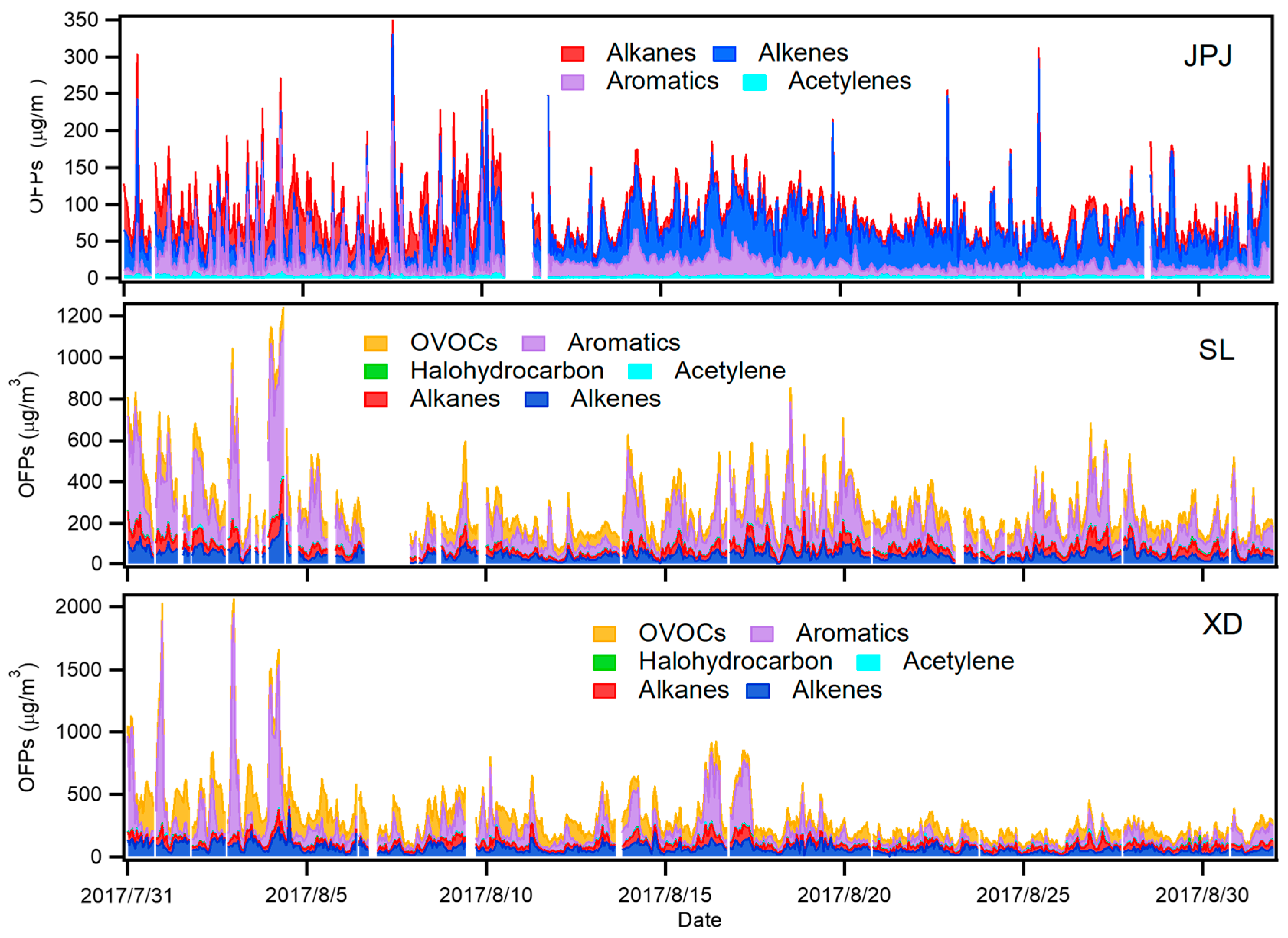
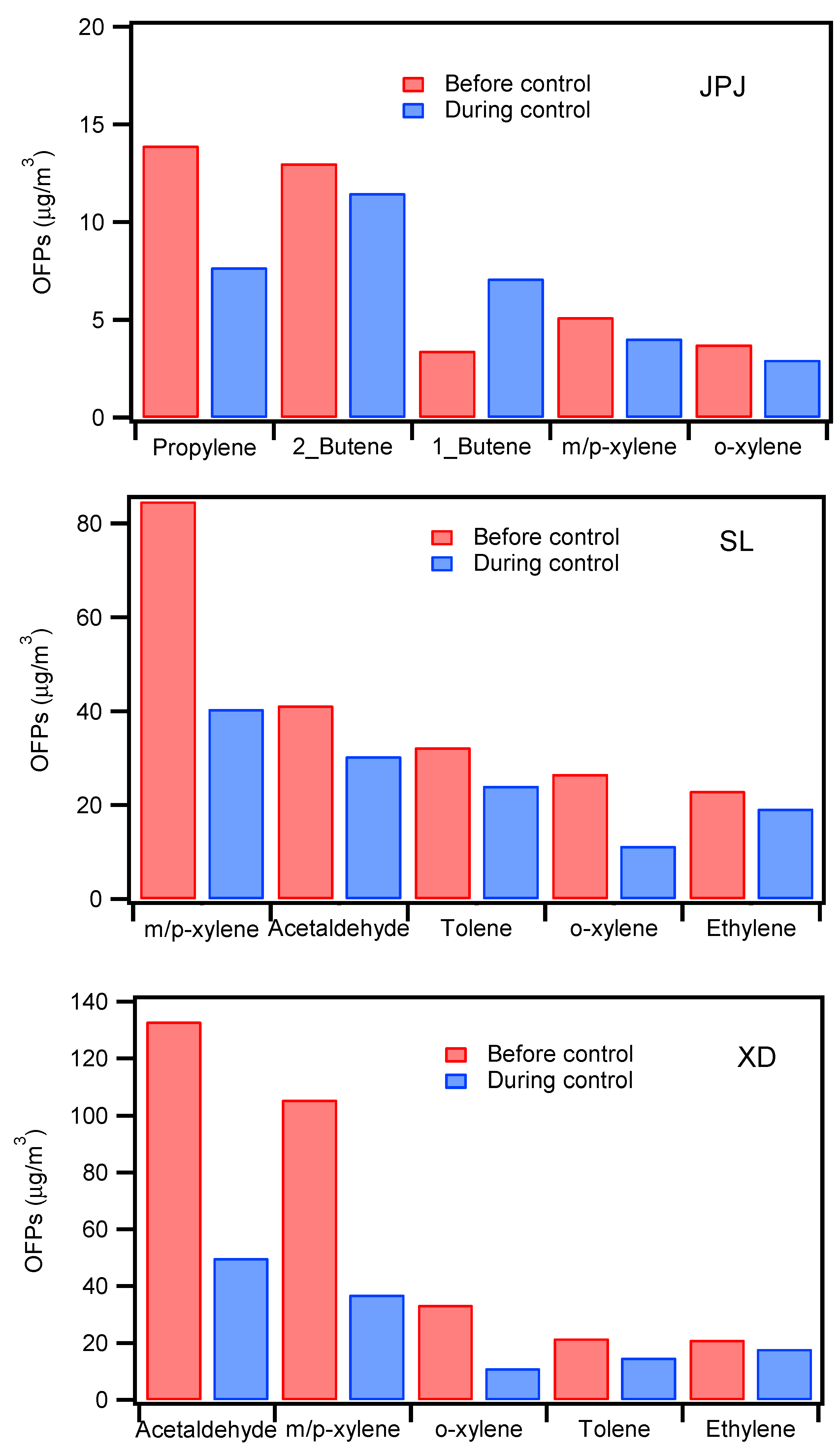
3.2. Contributions of Different Volatile Organic Compounds to Ozone Formation

As the main precursors of ozone, VOCs and NOx are directly associated with O3 production, but have a complex relationship with each other. Therefore, O3 formation from VOCs has been further studied by using the OFP method which was introduced in the methodology section to assess the relationship between VOC emission reduction and O3 formation.
The variations in OFPs of VOC sub-groups calculated from their concentrations at different sites are plotted in Figure 6, showing different characteristics compared with their mixing ratios (Figure 2). Aromatics were the most reactive species for ozone production at all the sites before control, mainly owing to the large averaged mixing ratios of toluene, ethylbenzene and xylene and their relatively high MIR values (Table S4 of the Supplementary Materials). In addition, acetaldehyde mixing ratios could reach ~10 ppbv before control at XD, which caused a higher contribution of OVOCs relative to OFPs. Although alkenes were always reactive species in different regions, their contributions to OFPs were higher at JPJ, due to higher mixing ratios detected during the control period. Aldehydes, toluene, and m/p-xylene made the largest contribution to the total OFPs at different sites. Their high photochemistry reactivity and concentrations ensured that they were the largest contributors to ozone formation in the city, accounting for 9.61–23.7%, 11.7–22.0%, and 11.7–22.0% of the overall OFPs, respectively. Ethylene, propylene and isopentane were also key species in the formation of ozone at all the sites.
The top five OFP values calculated from the averaged VOC species concentrations at different sites are displayed in Figure 7. The top five reactive species for O3 formation contributed to around 37% of OFPs at JPJ, 57% at SL, and 56% at XD. At different sites, the most significant contributors to O3 formation were similar. In general, aromatics, OVOCs, and olefins contributed most to the total OFP, because of their large MIR values and high concentrations. However, the mitigation options presented various results at each site. At SL, which is close to industrial areas where xylene concentrations had been cut around 50%, suggesting that the use status of organic solvents in factories were well controlled. Cleaning up and remediation of “scattered and polluted” enterprises and limiting emissions produced a marked effect. At XD, acetaldehyde contributed most to ozone formation during the whole period, although it decreased by about 50%, implying that the elimination of heavily polluted vehicles efficiently decreased VOCs emission and then slowed down the formation of secondary pollutants.
Although the OFP values varied dramatically at the above sites, the species with the highest OFP were almost the same at all three sites. At JPJ in the city center, the concentration of xylene was lower than the other two sites, whereas alkenes, such as propene and butene mostly produced by LPG combustion, became the major contributors of O3 formation. Because OVOCs were not monitored at JPJ, it was difficult to justify the limited regime and to estimate the real contribution of each VOC species to the local formation of ground-level ozone.
In Chengdu, ozone generation is generally controlled by VOCs based on the observation of the model of O3-NOx-VOCs sensitivity analysis investigations [12]. However, to develop a specific VOCs-NOx control scheme, a series of sensitivity experiments and source analyses are needed to determine the key VOC species that affect ozone production and the collaborative control ratio of NOx to VOCs, and more work is needed to formulate the following control measurement. As mentioned above, the highly ranked species obtained using the OFP method were aldehyde, toluene, m/p-xylene, ethylene, propene and butene, which were closely associated with the use of solvents and petrochemicals. They were considered to play significant roles in O3 formation in and around city center. This suggests that controlling evaporative emissions from solvent use and petrochemical industry in special zones would likely to have a more positive impact on O3 abatement in Chengdu. Giving priority to reducing emissions of these ozone-reactive VOCs in different regions could help to mitigate regional O3 contamination in the whole city.

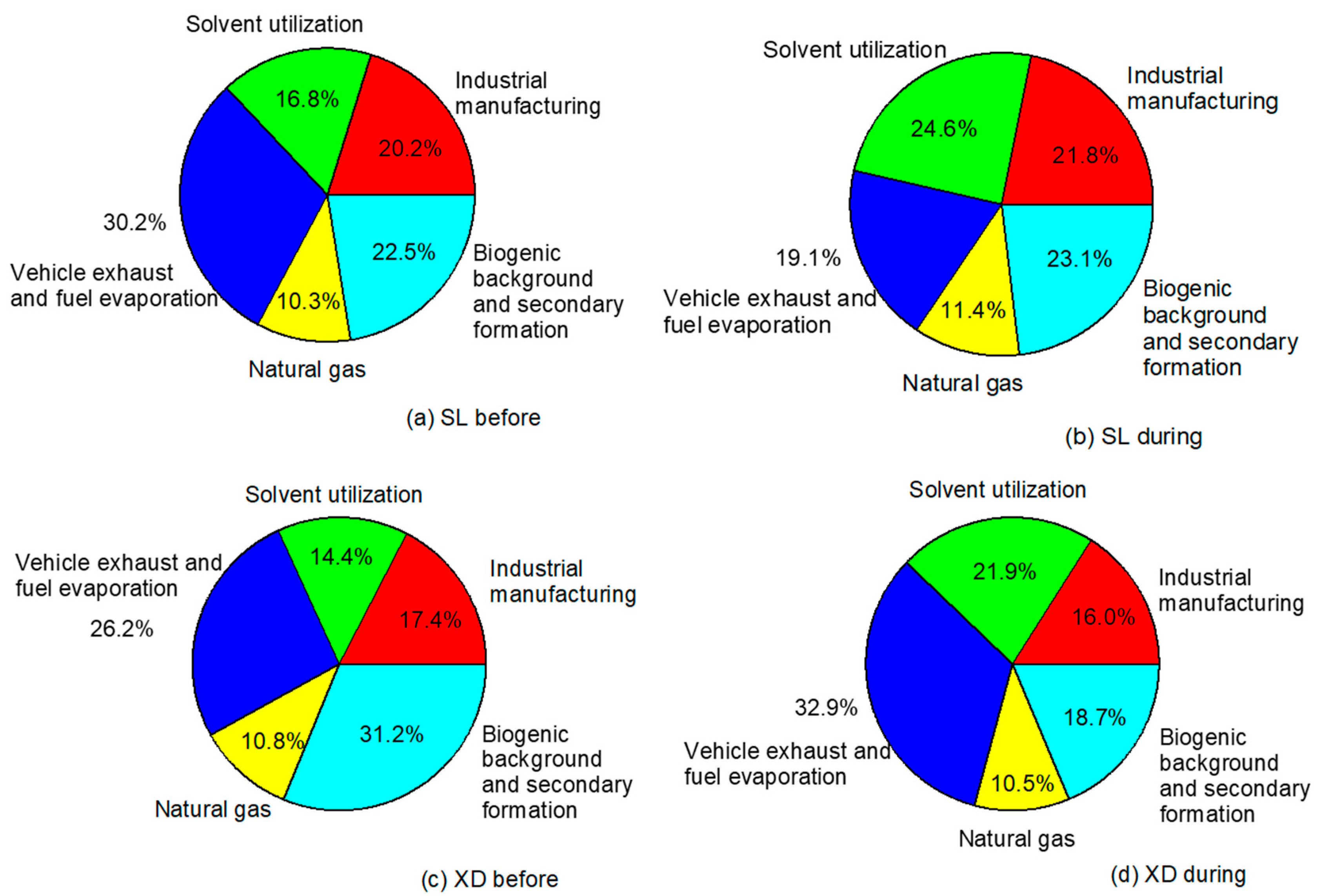
3.3. Comparison of VOC Sources before and during Control Period

In this work, PMF model (US EPA PMF 5.0) was applied to apportion the sources of VOCs at each study site and determine the predominant sources at different receptor sites. The VOC concentrations used in the model were separated into before and during control period in each site, thus different results would reflect the effect of control measures on emissions and help us evaluate these control strategies.
According to the model input signal-to-noise ratio, 17 species were classified as “bad”, 7 species were defined as “weak”, and 75 as “strong”. After the diagnostic test, the final analysis yielded five factors, namely (1) industrial manufacturing (2) solvent utilization (3) vehicle exhaust and fuel evaporation (4) natural gas (5) biogenic background and secondary formation. These sources were identified by related tracers listed in Table S5 of the Supplementary Materials.
The speciation profile of Factor 1 (Figure 8a) exhibited high contributions of dichloromethane, acetonitrile, and aromatics. There were higher chlorinated hydrocarbons in Factor 1. Chlorohydrocarbons were commonly used as the tracers of industrial and process emission sources [34], therefore we defined Factor 1 as industrial manufacturing sources.
The profile of Factor 2 (Figure 8b) had a high contribution from benzene series such as toluene, xylene, styrene, with more than 50% of their variabilities explained. These compounds are good markers for solvents [5]. Therefore, this source was considered as solvent utilization
The chemical profile of Factor 3, shown in Figure 8c, was mainly dominated by acetylene with approximately 80% of its variability explained. In addition, propane and iso-/n-butanes, pentanes, and light alkenes variabilities were explained on average 50% by this factor. In light of the tracers for fuel combustion from vehicles MTBE (methyl tert-butyl ether), it was identified as vehicle exhaust and fuel evaporation source.
The profile of Factor 4 (see Figure 8d) was mainly dominated by ethane, propane, and light alkanes, which are key long-lived compounds known to be associated with natural gas leakages. According to previous natural gas experiment [35], this profile was regarded as natural gas utilization.
The profile of Factor 5, shown in Figure 8e, presented a high contribution from isoprene and its oxidation product methyl vinyl ketone (MVK), which are known chemical markers of biogenic emissions, with more than 80% of their variability explained by this factor. In addition, this factor profile also included secondary oxidization products associated with a large contribution of selected OVOCs (acetaldehyde, acetone). Significant contributions from regional background such as Freon 114 and Freon 11, which have relatively long atmospheric residence times, were also observed. Therefore, this factor was defined as biogenic background and secondary formation source.
Figure 9 shows the source contributions of the two sites before and during the control period. Vehicular exhaust and fuel evaporation were found to be the most significant contributors to the TVOCs at the SL site before the implementation of control measures, with average contributions of 30.2%, followed by biogenic emission and secondary formation (22.5%), industrial manufacturing (20.2%), and solvent utilization (16.8%). These results are similar to our previous results observed in summer 2016 around this region [11]. During the control period (Figure 9b), the largest contribution was from solvent utilization (24.6%), while the proportion of biogenic emission and secondary formation, and industrial manufacturing was not much different, accounting for 23.1% and 21.8%, respectively. They were followed by vehicular exhaust and fuel evaporation (19.1%) and natural gas utilization (11.4%). This result revealed that the control measurement reduced the vehicular exhaust efficiently. According to the source profile, the concentration of long-chain alkanes which were associated with diesel exhaust (n-decane, n-undecane and n-dodecane) were controlled effectively.
At the XD site, the significant change related to the control strategy was the concentration of secondary formation VOCs decreasing, as shown in Figure 9c,d. Acetaldehyde and acetone were the main products through reactive VOCs with different oxidants, such as HOx, ROx radicals, NO3 radicals, O3, etc. The reduction in secondary pollutants accounted for the efficient reduction in reactive VOC species from primary emissions. The XD monitoring site was located in a busy logistic region, therefore the largest contributor to VOCs was vehicle emissions, which was expected. Furthermore, the solvent utilization also occupied a higher proportion in this area.

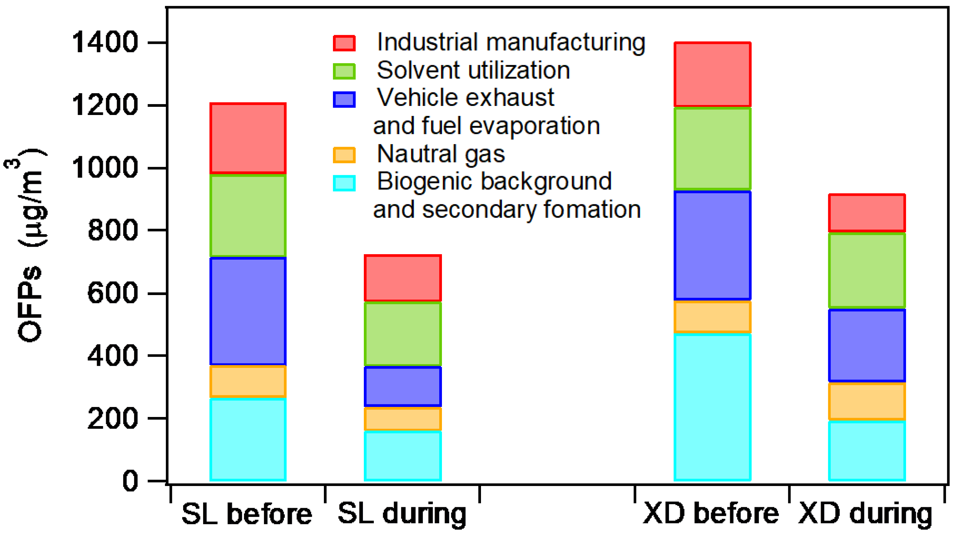
3.4. Contributions of VOC Sources to O3 Formation before and during the Performed Control Measures

The relative contributions of individual VOC sources and related VOC species to OFP at SL and XD using PMF are exhibited in Figure 10. Vehicular exhaust and fuel evaporation were found to be the largest OFPs contributors at SL (~1232 μg/m3, 28.0%) when the control measures were not implemented, followed by solvent utilization and biogenic background and secondary formation (~266 μg/m3, 21.6%), industrial manufacturing (~230 μg/m3, 18.7%) and natural gas utilization (~104 μg/m3, 8.4%). This was reasonable, because reactive VOC species, such as alkenes, aromatics, and long-chain alkanes, which have relatively high O3 formation reactivity, are abundant in vehicle exhausts and fuel evaporation. During the control period, heavy-polluting vehicles had been cleaned up off the road, the emission from industrial manufacturing was also well controlled, and solvent utilization became the largest source of O3 formation (~206 μg/m3, 28.1%). Therefore, it became apparent that minimizing VOC emissions from solvent utilization and industrial manufacturing would lower O3 formation in the southern part of Chengdu.
At the XD site, biogenic background and secondary formation were the dominant VOC sources of the total OFPs before control. Due to the emission reduction in active species, the concentration of reactive secondary pollutants (aldehyde compounds) showed evident decreases during the control period. This revealed that targeting active species and cutting down their emissions could achieve a multiplier effect. On the basis of mass concentrations of individual species in each source, m/p-xylene and toluene in solvent utilization and vehicular emissions; propene, ethene, toluene, and m/p-xylene in diesel vehicular emissions; and o-xylene;1,2,4-trimethylbenzene and ethene in industrial emissions were the dominant species from VOC emissions contributing to photochemical O3 formation. Thus, more attention should be given to a small number of reactive VOC species in order to achieve a more efficient control effect on O3 formation.

4. Conclusions and Long-Term Countermeasures

To effectively control photochemical pollution in summer, Chengdu government performed a strict control of atmospheric pollution act for one month between August 7 and September 7, 2017. In order to evaluate the control effect on regional contamination, field measurements at three urban sites (SL, XD, JPJ) of Chengdu were conducted to investigate the characteristics of O3 producers before and during control periods. Spatial and temporal distribution of ambient air pollutants before and during the control periods showed that the control had a significant effect on O3, cutting its concentration by at least 20%. Alkanes were the dominant VOC group observed at all the three study sites, followed by OVOCs, aromatics, halohydrocarbons and alkenes. There existed distinct diurnal variability patterns for different VOC groups, influenced by local emissions, meteorology and chemical reactions. Five dominant VOC sources were identified at the SL and XD sites using a PMF model.
The quantitative assessment of the contributions from different modeled sources presented in this study could provide an independent evaluation of the quality and the relevance of corresponding emission inventories. Therefore, the improvement of emission inventory will be very valuable to distinguish the discrepancies of local emission characteristics. Through considering both the abundance and maximum incremental reactivity of individual VOC species in each source, the OFP values identified vehicular and industrial emissions, particularly acetaldehyde m/p-xylene, toluene and propene, as the main contributors of O3 pollution. From this study, we found that cleaning up heavy-polluting vehicles, regulating disorderly emissions, and using clean energy were efficient measurements. Therefore, controlling overall pollutant emission (e.g., reducing total VOCs) should be gradually changed to targeting active VOC species.
Ozone pollution is a regional environmental issue rather than just a local pollution problem. From a regional perspective, it is suggested that appropriate ratios of VOC-NOx, their associated sensitivity to O3 formation, and relative benefits and disadvantages of reducing VOC-NOx should be continuedly investigated and evaluated. More studies based on long-term monitoring are necessary to determine the costs, benefits and performance of each pollution mitigation policy, and further in-depth research should be conducted on ozone pollution prevention and management to advance air quality improvement in the future.

Supplementary Materials

The following are available online at https://www.mdpi.com/2073-4433/11/12/1278/s1, Figure S1: Temporal profiles of temperature and relative humidity (RH) during study period. Figure S2: Wind direction and wind speed before (a) and during (b) the enforcement period. Table S1: The detection limits of measured VOCs by using online GC-FID/MS system. Table S2: Average meteorological condition before and during control periods in Chengdu. Table S3: The averaged mixing ratio of the measured species before and during control periods at each monitoring site. Table S4: MIR values derived from study by Carter. Table S5: VOC emission sources and corresponding tracers used in PMF source apportionment.

Author Contributions

Conceptualization, L.Z. and F.Y.; methodology, Q.T. and L.Z.; software, L.Z. and H.L.; validation, Q.T.; formal analysis, L.Z. and H.L.; investigation, Q.T.; data curation, Q.T., H.L. and M.F.; writing—original draft preparation, Q.T. and L.Z.; writing—review and editing, H.L., F.Y., W.J. and F.W.; supervision, Y.Q., F.Y., W.J. and F.W.; funding acquisition, L.Z. and F.Y. All authors have read and agreed to the published version of the manuscript.

Funding

This research was funded by the National Key R&D Program of China (No. 2018YFC0214004), Fundamental Research Funds for the Central Universities, grant number YJ201937 and YJ201891 and Chengdu Science and Technology Bureau, grant number 2020-YF09-00051-SN.

Acknowledgments

We are grateful for financial support from the National Key R&D Program of China (No. 2018YFC0214004), Fundamental Research Funds for the Central Universities, grant number YJ201937 and YJ201891 and Chengdu Science and Technology Bureau, grant number 2020-YF09-00051-SN. We would also like to show deep thankfulness to the reviewers and editors who have contributed valuable comments to improve the quality of the paper.

Conflicts of Interest

The authors declare no conflict of interest.

References

  1. Wang, T.; Xue, L.; Brimblecombe, P.; Lam, Y.F.; Li, L.; Zhang, L. Ozone pollution in China: A review of concentrations, meteorological influences, chemical precursors, and effects. Sci. Total Environ. 2017, 575, 1582–1596. [Google Scholar] [CrossRef]
  2. Zhao, Q.Y.; Bi, J.; Liu, Q.; Ling, Z.H.; Shen, G.F.; Chen, F.; Qiao, Y.Z.; Li, C.Y.; Ma, Z.W. Sources of volatile organic compounds and policy implications for regional ozone pollution control in an urban location of Nanjing, East China. Atmos. Chem. Phys. 2020, 20, 3905–3919. [Google Scholar] [CrossRef] [Green Version]
  3. He, Z.R.; Wang, X.M.; Ling, Z.H.; Zhao, J.; Guo, H.; Shao, M.; Wang, Z. Contributions of different anthropogenic volatile organic compound sources to ozone formation at a receptor site in the Pearl River Delta region and its policy implications. Atmos. Chem. Phys. 2019, 19, 8801–8816. [Google Scholar] [CrossRef] [Green Version]
  4. Shi, G.; Yang, F.; Zhang, L.; Zhao, T.; Hu, J. Impact of Atmospheric Circulation and Meteorological Parameters on Wintertime Atmospheric Extinction in Chengdu and Chongqing of Southwest China during 2001–2016. Aerosol Air Qual. Res. 2019, 19, 1538–1554. [Google Scholar] [CrossRef] [Green Version]
  5. Yang, X.Y.; Wu, K.; Wang, H.L.; Liu, Y.M.; Gu, S.; Lu, Y.Q.; Zhang, X.L.; Hu, Y.S.; Ou, Y.H.; Wang, S.G.; et al. Summertime ozone pollution in Sichuan Basin, China: Meteorological conditions, sources and process analysis. Atmos. Environ. 2020, 226, 117392. [Google Scholar] [CrossRef]
  6. Yang, F.; Tan, J.; Zhao, Q.; Du, Z.; He, K.; Ma, Y.; Duan, F.; Chen, G.; Zhao, Q. Characteristics of PM2.5 speciation in representative megacities and across China. Atmos. Chem. Phys. 2011, 11, 5207–5219. [Google Scholar] [CrossRef] [Green Version]
  7. Wang, Y.; Zhang, Y.; Hao, J.; Luo, M. Seasonal and spatial variability of surface ozone over China: Contributions from background and domestic pollution. Atmos. Chem. Phys. 2011, 11, 3511–3525. [Google Scholar] [CrossRef] [Green Version]
  8. Deng, Y.; Li, J.; Li, Y.; Wu, R.; Xie, S. Characteristics of volatile organic compounds, NO2, and effects on ozone formation at a site with high ozone level in Chengdu. J. Environ. Sci. 2019, 75, 334–345. [Google Scholar] [CrossRef]
  9. Li, Y.P.; Fan, Z.Y.; Pu, M.; Zhang, J.L.; Yang, Z.Z.; Wu, D. Pollution Characteristics and Health Risk Assessment of Atmospheric VOCs in Chengdu. Environ. Sci. 2018, 39, 9. [Google Scholar] [CrossRef]
  10. Xu, C.X.; Han, L.; Wang, B.; Wang, J.Q. Analyses of Pollution Characteristics, Ozone Formation Potential and Sources of VOCs Atmosphere in Chengdu City in Summer 2017. Res. Environ. Sci. 2019, 32, 8. [Google Scholar]
  11. Tan, Q.; Liu, H.; Xie, S.; Zhou, L.; Song, T.; Shi, G.; Jiang, W.; Yang, F.; Wei, F. Temporal and spatial distribution characteristics and source origins of volatile organic compounds in a megacity of Sichuan Basin, China. Environ. Res. 2020, 185, 109478. [Google Scholar] [CrossRef] [PubMed]
  12. Tan, Z.; Lu, K.; Jiang, M.; Su, R.; Dong, H.; Zeng, L.; Xie, S.; Tan, Q.; Zhang, Y. Exploring ozone pollution in Chengdu, southwestern China: A case study from radical chemistry to O-3-VOC-NOx sensitivity. Sci. Total Environ. 2018, 636, 775–786. [Google Scholar] [CrossRef] [PubMed]
  13. Song, M.; Tan, Q.; Feng, M.; Qu, Y.; Liu, X.; An, J.; Zhang, Y. Source Apportionment and Secondary Transformation of Atmospheric Nonmethane Hydrocarbons in Chengdu, Southwest China. J. Geophys. Res. Atmos. 2018, 123, 9741–9763. [Google Scholar] [CrossRef]
  14. Song, M.; Liu, X.; Tan, Q.; Feng, M.; Qu, Y.; An, J.; Zhang, Y. Characteristics and formation mechanism of persistent extreme haze pollution events in Chengdu, southwestern China. Environ. Pollut. 2019, 251, 1–12. [Google Scholar] [CrossRef] [PubMed]
  15. Li, B.; Ho, S.S.H.; Gong, S.; Ni, J.; Li, H.; Han, L.; Yang, Y.; Qi, Y.; Zhao, D. Characterization of VOCs and their related atmospheric processes in a central Chinese city during severe ozone pollution periods. Atmos. Chem. Phys. 2019, 19, 617–638. [Google Scholar] [CrossRef] [Green Version]
  16. Zhang, Q.; Yuan, B.; Shao, M.; Wang, X.; Lu, S.; Lu, K.; Wang, M.; Chen, L.; Chang, C.C.; Liu, S.C. Variations of ground-level O-3 and its precursors in Beijing in summertime between 2005 and 2011. Atmos. Chem. Phys. 2014, 14, 6089–6101. [Google Scholar] [CrossRef] [Green Version]
  17. Di Carlo, P.; Brune, W.H.; Martinez, M.; Harder, H.; Lesher, R.; Ren, X.R.; Thornberry, T.; Carroll, M.A.; Young, V.; Shepson, P.B.; et al. Missing OH reactivity in a forest: Evidence for unknown reactive biogenic VOCs. Science 2004, 304, 722–725. [Google Scholar] [CrossRef]
  18. Zhang, K.; Li, L.; Huang, L.; Wang, Y.J.; Huo, J.T.; Duan, Y.S.; Wang, Y.H.; Fu, Q.Y. The impact of volatile organic compounds on ozone formation in the suburban area of Shanghai. Atmos. Environ. 2020, 232. [Google Scholar] [CrossRef]
  19. Wang, B.; Shao, M.; Lu, S.H.; Yuan, B.; Zhao, Y.; Wang, M.; Zhang, S.Q.; Wu, D. Variation of ambient non-methane hydrocarbons in Beijing city in summer 2008. Atmos. Chem. Phys. 2010, 10, 5911–5923. [Google Scholar] [CrossRef] [Green Version]
  20. Hu, B.; Xu, H.; Deng, J.; Yi, Z.; Chen, J.; Xu, L.; Hong, Z.; Chen, X.; Hong, Y. Characteristics and Source Apportionment of Volatile Organic Compounds for Different Functional Zones in a Coastal City of Southeast China. Aerosol Air Qual. Res. 2018, 18, 2840–2852. [Google Scholar] [CrossRef]
  21. Zhang, H.; Li, H.; Zhang, Q.; Zhang, Y.; Zhang, W.; Wang, X.; Bi, F.; Chai, F.; Gao, J.; Meng, L.; et al. Atmospheric Volatile Organic Compounds in a Typical Urban Area of Beijing: Pollution Characterization, Health Risk Assessment and Source Apportionment. Atmosphere 2017, 8, 61. [Google Scholar] [CrossRef] [Green Version]
  22. Li, L.; Xie, S.; Zeng, L.; Wu, R.; Li, J. Characteristics of volatile organic compounds and their role in ground-level ozone formation in the Beijing-Tianjin-Hebei region, China. Atmos. Environ. 2015, 113, 247–254. [Google Scholar] [CrossRef]
  23. Zhu, Y.; Yang, L.; Chen, J.; Wang, X.; Xue, L.; Sui, X.; Wen, L.; Xu, C.; Yao, L.; Zhang, J.; et al. Characteristics of ambient volatile organic compounds and the influence of biomass burning at a rural site in Northern China during summer 2013. Atmos. Environ. 2016, 124, 156–165. [Google Scholar] [CrossRef]
  24. Carter, W.P.L. Development of the SAPRC-07 chemical mechanism. Atmos. Environ. 2010, 44, 5324–5335. [Google Scholar] [CrossRef]
  25. Li, J.; Zhai, C.; Yu, J.; Liu, R.; Li, Y.; Zeng, L.; Xie, S. Spatiotemporal variations of ambient volatile organic compounds and their sources in Chongqing, a mountainous megacity in China. Sci. Total Environ. 2018, 627, 1442–1452. [Google Scholar] [CrossRef]
  26. Wang, F.; Zhang, Z.; Acciai, C.; Zhong, Z.; Huang, Z.; Lonati, G. An Integrated Method for Factor Number Selection of PMF Model: Case Study on Source Apportionment of Ambient Volatile Organic Compounds in Wuhan. Atmosphere 2018, 9, 390. [Google Scholar] [CrossRef] [Green Version]
  27. Huang, Y.S.; Hsieh, C.C. Ambient volatile organic compound presence in the highly urbanized city: Source apportionment and emission position. Atmos. Environ. 2019, 206, 45–59. [Google Scholar] [CrossRef]
  28. Hui, L.R.; Liu, X.G.; Tan, Q.W.; Feng, M.; An, J.L.; Qu, Y.; Zhang, Y.H.; Jiang, M.Q. Characteristics, source apportionment and contribution of VOCs to ozone formation in Wuhan, Central China. Atmos. Environ. 2018, 192, 55–71. [Google Scholar] [CrossRef]
  29. Zheng, H.; Kong, S.F.; Xing, X.L.; Mao, Y.; Hu, T.P.; Ding, Y.; Li, G.; Liu, D.T.; Li, S.L.; Qi, S.H. Monitoring of volatile organic compounds (VOCs) from an oil and gas station in northwest China for 1 year. Atmos. Chem. Phys. 2018, 18, 4567–4595. [Google Scholar] [CrossRef] [Green Version]
  30. Shao, P.; An, J.; Xin, J.; Wu, F.; Wang, J.; Ji, D.; Wang, Y. Source apportionment of VOCs and the contribution to photochemical ozone formation during summer in the typical industrial area in the Yangtze River Delta, China. Atmos. Res. 2016, 176, 64–74. [Google Scholar] [CrossRef]
  31. Chang, C.C.; Chen, T.Y.; Chou, C.; Liu, S.C. Assessment of traffic contribution to hydrocarbons using 2,2-dimethylbutane as a vehicular indicator. Terr. Atmos. Ocean. Sci. 2004, 15, 697–711. [Google Scholar] [CrossRef] [Green Version]
  32. Li, J.; Lu, K.; Lv, W.; Li, J.; Zhong, L.; Ou, Y.; Chen, D.; Huang, X.; Zhang, Y. Fast increasing of surface ozone concentrations in Pearl River Delta characterized by a regional air quality monitoring network during 2006–2011. J. Environ. Sci. 2014, 26, 23–36. [Google Scholar] [CrossRef]
  33. Chen, W.T.; Shao, M.; Lu, S.H.; Wang, M.; Zeng, L.M.; Yuan, B.; Liu, Y. Understanding primary and secondary sources of ambient carbonyl compounds in Beijing using the PMF model. Atmos. Chem. Phys. 2014, 14, 3047–3062. [Google Scholar] [CrossRef] [Green Version]
  34. Mo, Z.; Shao, M.; Lu, S.; Qu, H.; Zhou, M.; Sun, J.; Gou, B. Process-specific emission characteristics of volatile organic compounds (VOCs) from petrochemical facilities in the Yangtze River Delta, China. Sci. Total Environ. 2015, 533, 422–431. [Google Scholar] [CrossRef]
  35. Baudic, A.; Gros, V.; Sauvage, S.; Locoge, N.; Sanchez, O.; Sarda-Estève, R.; Kalogridis, C.; Petit, J.E.; Bonnaire, N.; Baisnée, D.; et al. Seasonal variability and source apportionment of volatile organic compounds (VOCs) in the Paris megacity (France). Atmos. Chem. Phys. 2016, 16, 11961–11989. [Google Scholar] [CrossRef] [Green Version]
Figure 1. The locations of the monitoring sites and their surrounding environment in Chengdu. The rose plot displays the wind speed and direction during the field campaign. SL, Shuangliu; XD, Xindu; JPJ, Junpingjie.
Atmosphere 11 01278 g001
Figure 2. Temporal profiles of O3, NO2 and CO concentrations at each site (red line: JPJ; blue line: SL; green line: XD). The horizontal dashed line in the first panel indicates the O3 standard Grade II, i.e., 160 μg/m3. The vertical dashed line represents when the control strategy was implemented.
Atmosphere 11 01278 g002
Figure 3. The diurnal profiles of O3, NO2, CO concentrations at each site before (red line: July 31–August 6) and during (blue line: August 7–August 31) control periods.
Atmosphere 11 01278 g003
Figure 4. Time series of volatile organic compounds (VOCs) observed at three monitoring sites in Chengdu; the dashed line represents when the control strategy was implemented.
Atmosphere 11 01278 g004
Figure 5. Diurnal variations of VOC groups observed at SL, XD and JPJ before (red line: July 31–August 6) and during (bule line: August 7–August 31) control periods.
Atmosphere 11 01278 g005
Figure 6. Contribution of various VOC groups to ozone formation potentials (OFPs) at each study site.
Atmosphere 11 01278 g006
Figure 7. Top five VOC species and their contribution to OFPs at each study site. (Red bar: before control; Blue bar: during control).
Atmosphere 11 01278 g007
Figure 8. Source profiles of VOCs identified using the positive matrix factorization (PMF) receptor model and the relative contributions of the individual VOC species (from the SL site before control). (ae) represent the characteristics of each source factor (Factor 1-Factor6). The name of each VOC species is listed in Table 2.
Atmosphere 11 01278 g008
Figure 9. Relative contributions of different sources to TVOC mixing ratios from August 1–7 (a,c, before control) and August 8–31 (b,d, during control) at the SL and XD monitoring sites.
Atmosphere 11 01278 g009
Figure 10. The contribution of individual sources to the total OFP of all sources extracted from PMF.
Atmosphere 11 01278 g010
Table 1. Mean value of O3 concentrations and ambient air pollutants before and during control periods at each monitoring site.
JPJSLXD
BeforeDuringBeforeDuringBeforeDuring
O3 (μg/m3)88.566.795.175.993.667.9
NO2 (μg/m3)45.034.232.724.523.921.2
CO (μg/m3)0.6800.5700.9100.7900.8800.760
TVOCs (ppbv)14.411.852.834.960.647.0
Alkanes (ppbv)10.06.2816.512.318.423.7
Alkenes (ppbv)0.892.573.772.794.463.12
Acetylene (ppbv)2.442.133.262.402.812.59
Aromatics(ppbv)1.010.797.854.417.273.32
OVOCs (ppbv)--13.37.6820.59.81
Halohydrocarbons(ppbv)--7.704.906.704.14
Notes: TVOCs is total volatile organic compounds measured in each site; OVOCs is oxygen-containing volatile organic compounds; - meant the values were not measured in this work.
Table 2. VOCs species applied in the PMF model.
Serial NumberVOC SpeciesSerial NumberVOC Species
1Acetaldehyde421,4-Dichlorobenzene
2Acrolein43Acetylene
3Propanal44Ethane
4Acetone45Propane
5MTBE46Isobutane
6Methacrolein47n-Butane
7n-Butanal48Cyclopentane
8Methylvinylketone49Isopentane
9Methylethylketone50n-Pentane
102-pentanone512,2-dimethylbutane
11n-Pentanal522,3-dimethylbutane
123-pentanone532-methylpentane
13Benzene543-methylpentane
14Toluene55n-hexane
15Ethylbenzene562,4-dimethylpentane
16m/p-xylene57methylcyclopentane
17o-xylene582-methylhexane
18Styrene59Cyclohexane
19isopropylbenzene602,3-dimethylpentane
20n-Propylbenzene613-methylhexane
213-ethyltoluene622,2,4-trimethylpentane
224-ethyltoluene63n-heptane
231,3,5-trimethylbenzene64Methylcyclohexane
242-ethyltoluene652,3,4-trimethylpentane
251,2,4-trimethylbenzene662-methylheptane
261,2,3-trimethylbenzene673-methylheptane
271,3-diethylbenzene68Octane
281,4-diethylbenzene69n-Nonane
29Freon11470n-decane
30Chloromethane71Udecane
31Vinylchloride72Dodecane
32Freon1173Ethylene
33Freon11374Propene
34Dichloromethane75trans-2-Butene
351,1-Dichloroethane761-Butene
36Chloroform771,3-Butadiene
37tetrachloromethane78trans-2-pentene
381,2-Dichloroethane79Isoprene
391,2-Dichloropropane801-hexene
40trans-1,3-Dichloropropene81Trichloroethylene
41Tetrachloroethylene82Acetonitrile
Publisher’s Note: MDPI stays neutral with regard to jurisdictional claims in published maps and institutional affiliations.

