Ammonia Emission Characteristics of a Mechanically Ventilated Swine Finishing Facility in Korea

 , , ,
, , ,
Abstract
:1. Introduction
2. Experiments
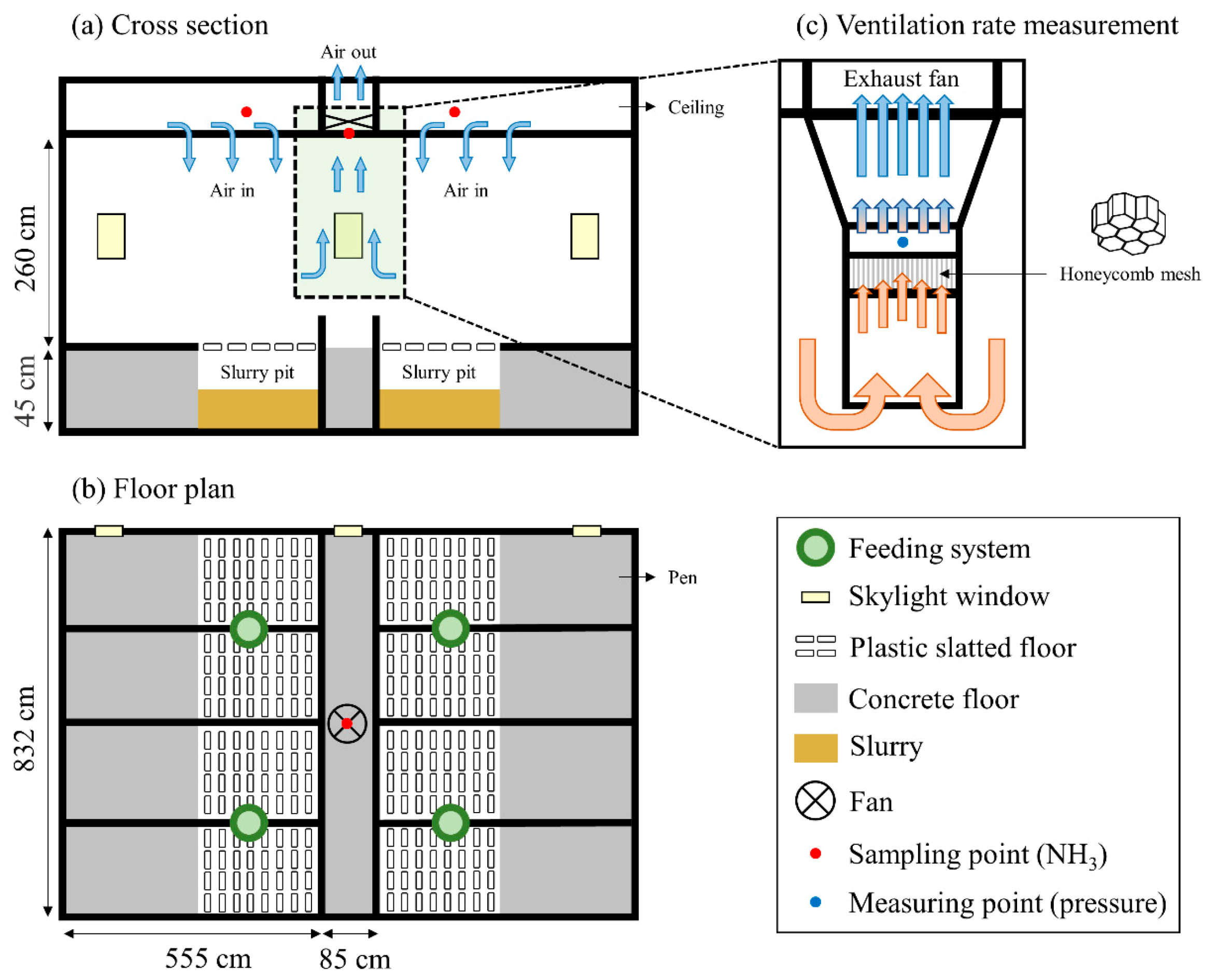
2.1. Housing
2.2. Animals
2.3. Measurements
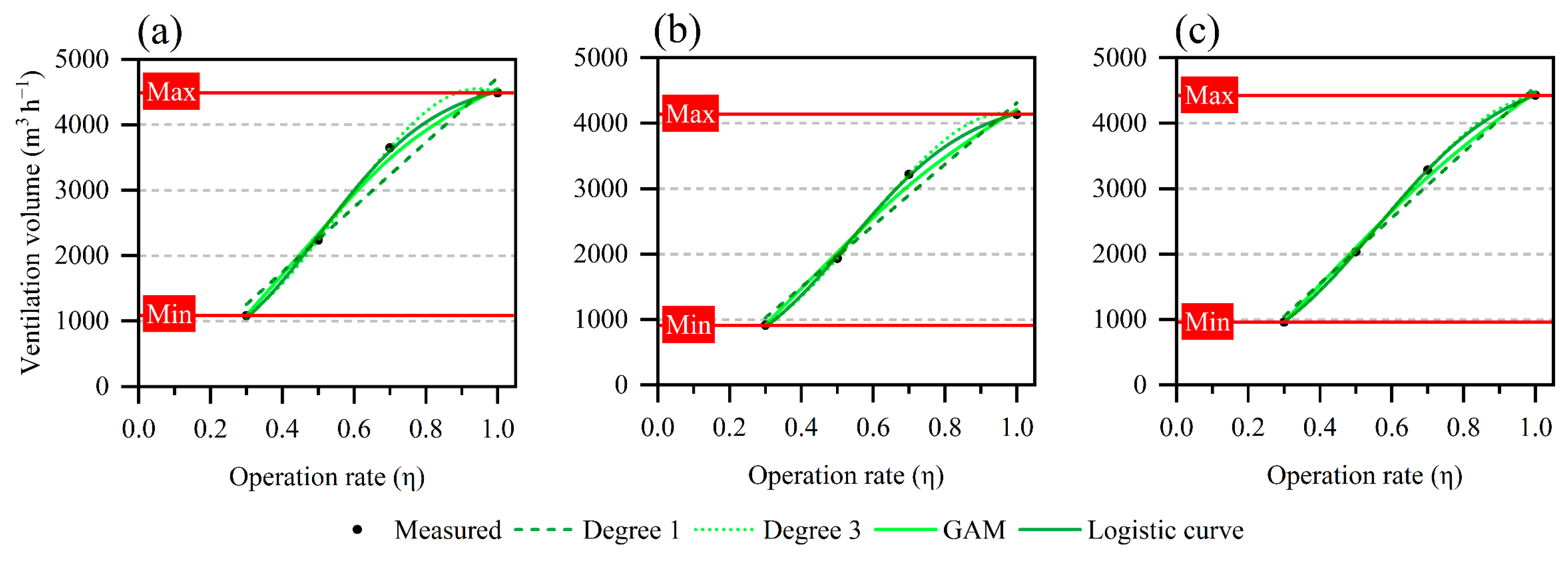
2.4. Data Analysis
3. Results and Discussion
3.1. Patterns of Ammonia Concentration, Ventilation Rate, Temperature, and Relative Humidity
3.2. Characteristics of Ammonia Emissions
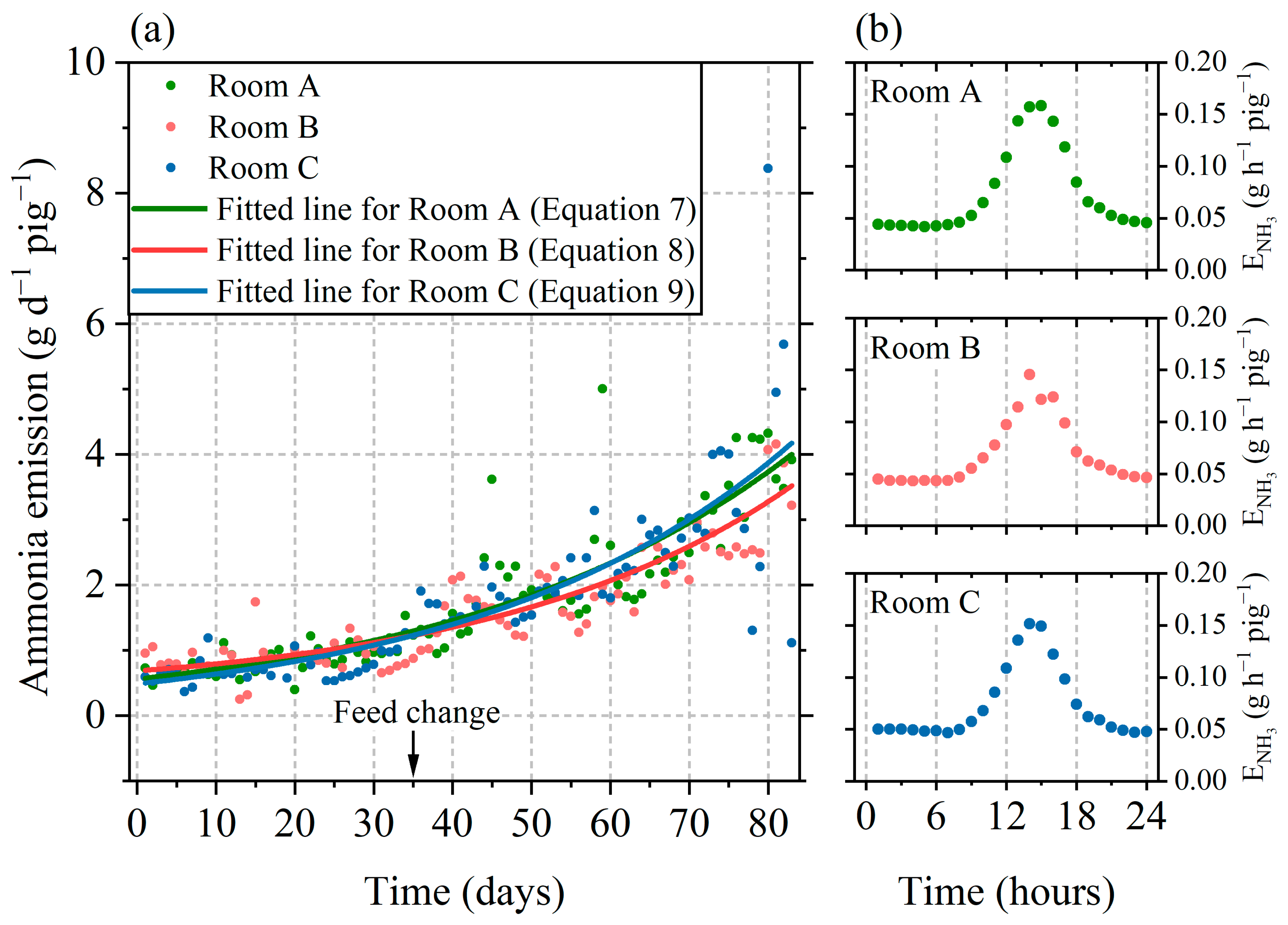
3.2.1. Time-Series and Diurnal Variation
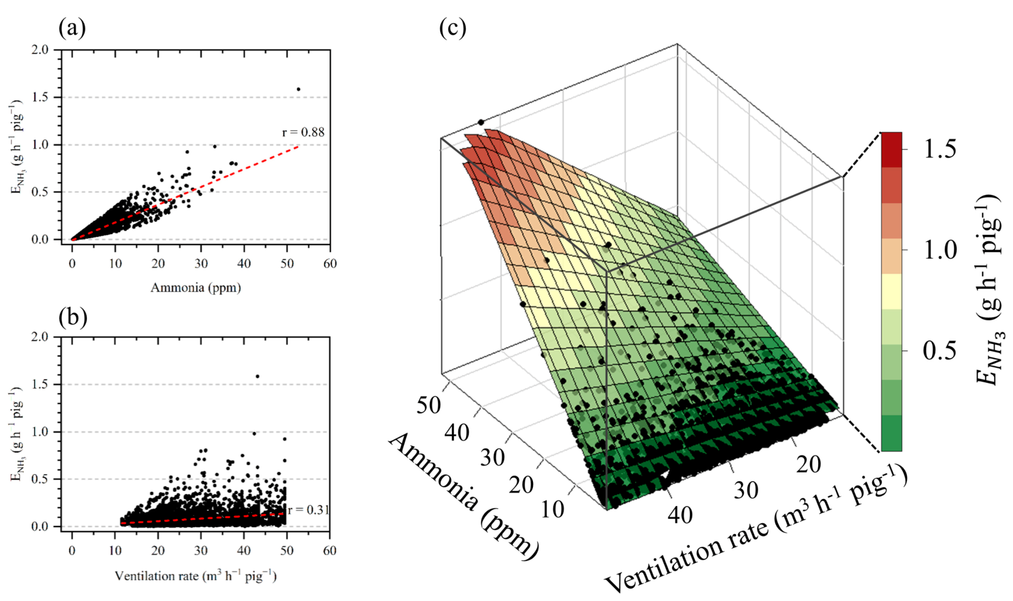
3.2.2. Correlation Analysis
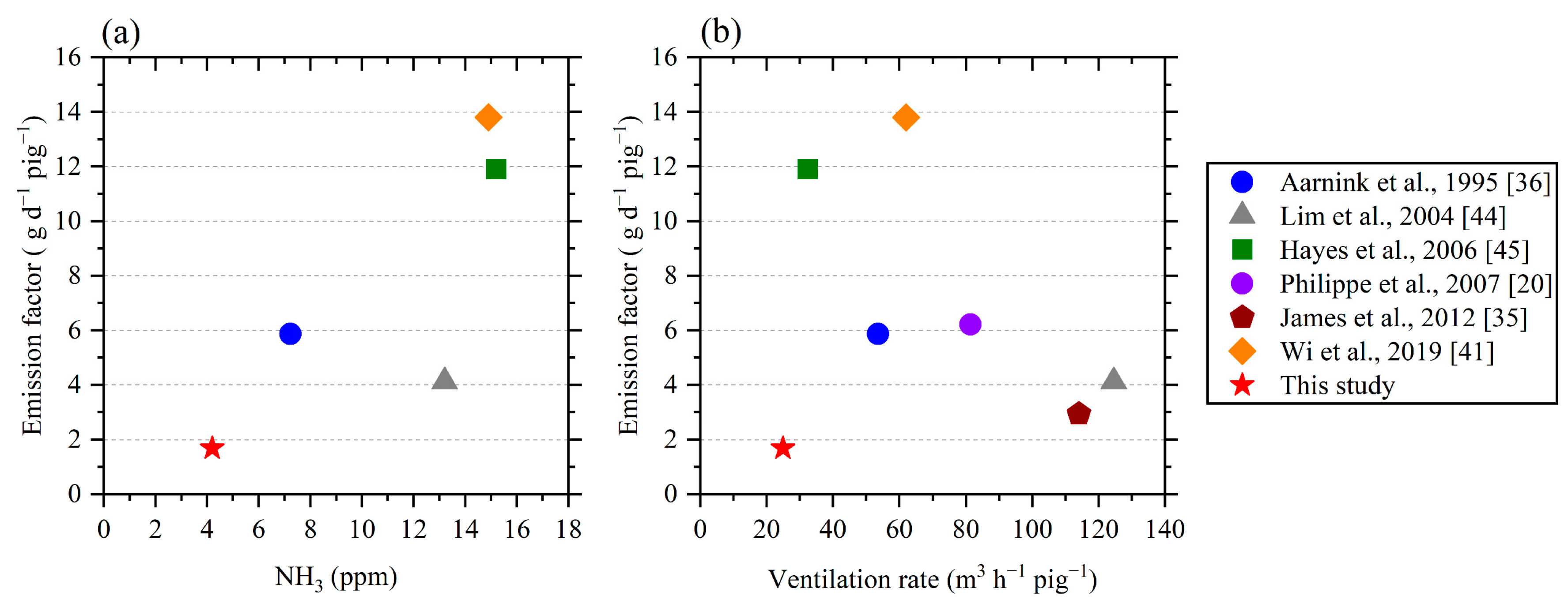
3.3. Emission Factor
4. Conclusions
Supplementary Materials
Author Contributions
Funding
Conflicts of Interest
References
- Denmead, O.T.; Chen, D.; Griffith, D.W.T.; Loh, Z.M.; Bai, M.; Naylor, T. Emissions of the indirect greenhouse gases NH3 and NOx from Australian beef cattle feedlots. Aust. J. Exp. Agric. 2008, 48, 213–218. [Google Scholar] [CrossRef]
- Ferm, M. Atmospheric ammonia and ammonium transport in Europe and critical loads: A review. Nutr. Cycl. Agroecosys. 1998, 51, 5–17. [Google Scholar] [CrossRef]
- Mosier, A.; Kroeze, C.; Nevison, C.; Oenema, O.; Seitzinger, S.; Van Cleemput, O. Closing the global N2O budget: Nitrous oxide emissions through the agricultural nitrogen cycle. Nutr. Cycl. Agroecosys. 1998, 52, 225–248. [Google Scholar] [CrossRef]
- Zhang, W.; Dou, Z.; He, P.; Ju, X.T.; Powlson, D.; Chadwick, D.; Norse, D.; Lu, Y.L.; Zhang, Y.; Wu, L.; et al. New technologies reduce greenhouse gas emissions from nitrogenous fertilizer in China. Proc. Natl. Acad. Sci. USA 2013, 110, 8375–8380. [Google Scholar] [CrossRef] [Green Version]
- Behera, S.N.; Sharma, M.; Aneja, V.P.; Balasubramanian, R. Ammonia in the atmosphere: A review on emission sources, atmospheric chemistry and deposition on terrestrial bodies. Environ. Sci. Pollut. Res. 2013, 20, 8092–8131. [Google Scholar] [CrossRef]
- Finlayson-Pitts, B.; Pitts, J. Chemistry of Upper and Lower Atmosphere, 1st ed.; Elsevier: Amsterdam, The Nederland, 2000. [Google Scholar]
- Agency for Toxic Substances and Disease Registry (ATSDR). Toxicological Profile for Ammonia; ATSDR: Atlanta, GA, USA, 2004.
- Hutchings, N.J.; Sommer, S.G.; Andersen, J.M.; Asman, W.A.H. A detailed ammonia emission inventory for Denmark. Atmos. Environ 2001, 35, 1959–1968. [Google Scholar] [CrossRef]
- Pozzer, A.; Tsimpidi, A.P.; Karydis, V.A.; De Meij, A.; Lelieveld, J. Impact of agricultural emission reductions on fine-particulate matter and public health. Atmos. Chem. Phys. 2017, 17, 12813–12826. [Google Scholar] [CrossRef] [Green Version]
- Battye, W.; Aneja, V.P.; Roelle, P.A. Evaluation and improvement of ammonia emissions inventories. Atmos. Environ. 2003, 37, 3873–3883. [Google Scholar] [CrossRef]
- Bouwman, A.F.; Lee, D.S.; Asman, W.A.H.; Dentener, F.J.; Van Der Hoek, K.W.; Olivier, J.G.J. A global high-resolution emission inventory for ammonia. Glob. Biogeochem. Cycles. 1997, 4, 561–587. [Google Scholar] [CrossRef]
- Huang, X.; Song, Y.; Li, M.; Li, J.; Huo, Q.; Cai, X.; Zhu, T.; Hu, M.; Zhang, H. A high-resolution ammonia emission inventory in China. Glob. Biogeochem. Cycles. 2012, 26, GB1030. [Google Scholar] [CrossRef]
- Lee, Y.H.; Park, S.U. Estimation of ammonia emission in South Korea. Water. Air. Soil Pollut. 2002, 135, 23–37. [Google Scholar] [CrossRef]
- Zhang, Y.; Dore, A.J.; Ma, L.; Liu, X.J.; Ma, W.Q.; Cape, J.N.; Zhang, F.S. Agricultural ammonia emissions inventory and spatial distribution in the North China Plain. Environ. Pollut. 2010, 158, 490–501. [Google Scholar] [CrossRef] [Green Version]
- National Institute of Environmental Research (NIER). 2016 National Air Pollutant Emissions; NIER: Incheon, Korea, 2019.
- Yeo, S.; Lee, H.; Choi, S.; Seol, S.; Jin, H.; Yoo, C.; Lim, J.; Kim, J. Analysis of the National Air Pollutant Emission Inventory (CAPSS 2015) and the major cause of change in Republic of Korea. Asian J. Atmos. Environ. 2019, 13, 212–231. [Google Scholar] [CrossRef]
- Arogo, J.; Westerman, P.W.; Heber, A.J. A review of ammonia emissions from confined swine feeding operations. Trans. Am. Soc. Agric. Eng. 2003, 46, 805–817. [Google Scholar] [CrossRef]
- National Institute of Environmental Research (NIER). Emissions Calculation and Inventory Building of Ammonia in the Atmosphere(II); NIER: Incheon, Korea, 2008.
- Philippe, F.-X.; Cabaraux, J.-F.; Nicks, B. Ammonia emissions from pig houses: Influencing factors and mitigation techniques. Agric. Ecosyst. Environ. 2011, 141, 245–260. [Google Scholar] [CrossRef]
- Philippe, F.-X.; Laitat, M.; Canart, B.; Vandenheede, M.; Nicks, B. Comparison of ammonia and greenhouse gas emissions during the fattening of pigs, kept either on fully slatted floor or on deep litter. Livest. Sci. 2007, 111, 144–152. [Google Scholar] [CrossRef]
- Hansen, M.J.; Nørgaard, J.V.; Adamsen, A.P.S.; Poulsen, H.D. Effect of reduced crude protein on ammonia, methane, and chemical odorants emitted from pig houses. Livest. Sci. 2014, 169, 118–124. [Google Scholar] [CrossRef]
- Verification of Environmental Technologies for Agricultural Production (VERA). Livestock Housing and Management Systems; International VERA Secretariat: Delft, The Nederland, 2018. [Google Scholar]
- Fundamentals, I.-P.; American Society of Heating, Refrigerating and Air-Conditioning Engineers (ASHRAE). ASHRAE Handbook; ASHRAE: Atlanta, GA, USA, 1993. [Google Scholar]
- Simmons, J.D.; Lott, B.D. Reduction of poultry ventilation fan output due to shutters. Appl. Eng. Agric. 1997, 13, 671–673. [Google Scholar] [CrossRef]
- Casey, K.D.; Gates, R.S.; Wheeler, E.F.; Xin, H.; Liang, Y.; Pescatore, A.J.; Ford, M.J. On-farm ventilation fan performance evaluations and implications. J. Appl. Poult. Res. 2008, 17, 283–295. [Google Scholar] [CrossRef]
- Alduchov, O.A.; Eskridge, R.E. Improved Magnus form approximation of saturation vapor pressure. J. Appl. Meteorol. 1996, 35, 601–609. [Google Scholar] [CrossRef]
- Sonntag, D. Important new values of the physical constants of 1986, vapour pressure formulations based on the ITS-90, and psychrometer formulae. Meteorol. Zeitschrift. 1990, 70, 340–344. [Google Scholar]
- Anderson, T.W.; Darling, D.A. Asymptotic Theory of Certain “Goodness of Fit” Criteria Based on Stochastic Processes. Ann. Math. Stat. 1952, 23, 193–212. [Google Scholar] [CrossRef]
- Shapiro, S.S.; Wilk, M.B. An Analysis of Variance Test for Normality (Complete Samples). Biometrika 1965, 52, 591–611. [Google Scholar] [CrossRef]
- Stephens, M.A. EDF Statistics for Goodness of Fit and Some Comparisons. J. Am. Stat. Assoc. 1974, 69, 730–737. [Google Scholar] [CrossRef]
- Mcdonald, J.H. Handbook of Biological Statistics, 3rd ed.; Sparky House Publishing: Baltimore, MD, USA, 2014. [Google Scholar]
- Blunden, J.; Aneja, V.P.; Westerman, P.W. Measurement and analysis of ammonia and hydrogen sulfide emissions from a mechanically ventilated swine confinement building in North Carolina. Atmos. Environ. 2008, 42, 3315–3331. [Google Scholar] [CrossRef]
- Heber, A.J.; Ni, J.Q.; Lim, T.T.; Diehl, C.A.; Sutton, A.L.; Duggirala, R.K.; Haymore, B.L.; Kelly, D.T.; Adamchuk, V.I. Effect of a manure additive on ammonia emission from swine finishing buildings. Trans. Am. Soc. Agric. Eng. 2000, 43, 1895–1902. [Google Scholar] [CrossRef] [Green Version]
- Zong, C.; Li, H.; Zhang, G. Ammonia and greenhouse gas emissions from fattening pig house with two types of partial pit ventilation systems. Agric. Ecosyst. Environ. 2015, 208, 94–105. [Google Scholar] [CrossRef]
- James, K.M.; Blunden, J.; Rumsey, I.C.; Aneja, V.P. Characterizing ammonia emissions from a commercial mechanically ventilated swine finishing facility and an anaerobic waste lagoon in North Carolina. Atmos. Pollut. Res. 2012, 3, 279–288. [Google Scholar] [CrossRef] [Green Version]
- Aarnink, A.J.A.; Keen, A.; Metz, J.H.M.; Speelman, L.; Verstegen, M.W.A. Ammonia emission patterns during the growing periods of pigs housed on partially slatted floors. J. Agric. Eng. Res. 1995, 62, 105–116. [Google Scholar] [CrossRef]
- Aarnink, A.J.A.; Van Den Berg, A.J.; Keen, A.; Hoeksma, P.; Verstegen, M.W.A. Effect of slatted floor area on ammonia emission and on the excretory and lying behaviour of growing pigs. J. Agric. Eng. Res. 1996, 64, 299–310. [Google Scholar] [CrossRef]
- Blanes-Vidal, V.; Hansen, M.N.; Pedersen, S.; Rom, H.B. Emissions of ammonia, methane and nitrous oxide from pig houses and slurry: Effects of rooting material, animal activity and ventilation flow. Agric. Ecosyst. Environ. 2008, 124, 237–244. [Google Scholar] [CrossRef]
- Costa, A. Ammonia Concentrations and Emissions from Finishing Pigs Reared in Different Growing Rooms. J. Environ. Qual. 2017, 46, 255–260. [Google Scholar] [CrossRef]
- Jeppsson, K.-H. Diurnal variation in ammonia, carbon dioxide and water vapour emission from an uninsulated, deep litter building for growing/finishing pigs. Biosyst. Eng. 2002, 81, 213–223. [Google Scholar] [CrossRef] [Green Version]
- Wi, J.; Lee, S.; Kim, E.; Lee, M.; Koziel, J.A.; Ahn, H. Evaluation of semi-continuous pit manure recharge system performance on mitigation of ammonia and hydrogen sulfide emissions from a swine finishing barn. Atmosphere 2019, 10, 170. [Google Scholar] [CrossRef] [Green Version]
- Grinn-Gofroń, A.; Bosiacka, B.; Bednarz, A.; Wolski, T. A comparative study of hourly and daily relationships between selected meteorological parameters and airborne fungal spore composition. Aerobiologia 2018, 34, 45–54. [Google Scholar] [CrossRef]
- Xia, S.; Mestas-Nunez, A.M.; Xie, H.; Vega, R. An Evaluation of Satellite Estimates of Solar Surface Irradiance Using Ground Observations in San Antonio, TX, USA. Remote Sens. 2017, 9, 1268. [Google Scholar] [CrossRef] [Green Version]
- Lim, T.T.; Heber, A.J.; Ni, J.-Q.; Kendall, D.C.; Richert, B.R. Effects of manure removal strategies on odor and gas emissions from swine finishing. Trans. Am. Soc. Agric. Eng. 2004, 47, 1–10. [Google Scholar] [CrossRef]
- Hayes, E.T.; Curran, T.P.; Dodd, V.A. Odour and ammonia emissions from intensive pig units in Ireland. Bioresour. Technol. 2006, 97, 940–948. [Google Scholar] [CrossRef] [Green Version]


| No. of Pigs | Finishing Periods(Days; Start/End) | Weight Range (kg) | Mean Feed Intake (kg d−1 pig−1) | Weight Gain (g d−1 Pig−1) | |
|---|---|---|---|---|---|
| Room A | 91 | 83; 15 August–5 November | 27.9–92.0 | 1.55 | 772 |
| Room B | 96 | 83; 22 August–12 November | 28.3–92.2 | 1.54 | 770 |
| Room C | 102 | 83; 29 August–19 November 19 | 27.1–90.4 | 1.43 | 763 |
| Average | 96 | 83 | 27.8–91.5 | 1.51 | 768 |
| Nutritional Content (%) | Finishing Period | |
|---|---|---|
| 1–35 Days | 36–83 Days | |
| Crude protein | 15.0 | 15.0 |
| Crude lipid | 3.0 | 4.0 |
| Crude fiber | 5.0 | 5.0 |
| Ash | 5.0 | 5.0 |
| Calcium | 0.6 | 0.5 |
| Phosphorus | 0.5 | 0.5 |
| Regression Model | Room A | Room B | Room C | |||
|---|---|---|---|---|---|---|
| RMSE a | MAPE b | RMSE | MAPE | RMSE | MAPE | |
| Degree 1 | 252 | 8.2% | 190 | 7.0% | 139 | 4.9% |
| Degree 3 | 0 | 0.0% | 0 | 0.0% | 0 | 0.0% |
| GAM c | 96 | 2.3% | 101 | 3.1% | 65 | 1.9% |
| Logistic curve | 47 | 2.1% | 28 | 1.5% | 3 | 0.2% |
| Ammonia Concentration (ppm) | Ventilation Rate (m3 h−1 pig−1) | Temperature (°C) | Relative Humidity (%) | |
|---|---|---|---|---|
| Room A | 3.60 ± 2.35 | 29.4 ± 6.1 | 24.1 ± 2.3 | 62.1 ± 7.3 |
| Room B | 4.23 ± 2.61 | 23.2 ± 5.0 | 24.0 ± 1.9 | 58.9 ± 9.6 |
| Room C | 4.73 ± 3.52 | 22.2 ± 5.1 | 23.7 ± 2.0 | 55.2 ± 10.7 |
| Average | 4.19 ± 2.91 | 24.9 ± 6.3 | 23.9 ± 2.1 | 58.8 ± 9.7 |
| Ammonia Concentration | Temperature | Relative Humidity | Ventilation Rate | |
|---|---|---|---|---|
| Temperature | −0.66 a | |||
| <0.001 b | ||||
| Relative humidity | −0.41 | 0.71 | ||
| <0.001 | <0.001 | |||
| Ventilation rate | −0.13 | 0.58 | 0.62 | |
| <0.001 | <0.001 | <0.001 | ||
| Ammonia emission | 0.88 | −0.37 | −0.12 | 0.31 |
| <0.001 | <0.001 | <0.001 | <0.001 |
| Reference | Growing Length | No. of Pigs | Weight (kg) | Ammonia a (ppm) | Temperature (°C) | Ventilation Rate b (m3 h−1 pig−1) | Emission Factor (g d−1 pig−1) | Floor Type c |
|---|---|---|---|---|---|---|---|---|
| [36] d | 104 days | 36 | 25.0–111.1 | 7.22 | 23.0 | 53.5 | 5.87 | PS (25%) |
| [44] e | 82 days | 25 | 88 | 13.2 | 25.0 | 124.6 | 4.12 | FS |
| [45] f | – | 300 | 35– | 15.2 | – | 32.4 | 11.9 | FS |
| [20] | 4 months | 80 | 23.8–111.7 | – | 20.5 | 81.4 | 6.22 | FS |
| [35] g | 9 days | 885 | 48.7 | – | 26.0 | 114.1 | 2.94 | – |
| [41] h | 14 days | 240 | 80 | 14.9 | 25.0 | 62.0 | 13.8 | FS |
| This study i | 83 days | 96 | 27.8–91.5 | 4.19 | 23.9 | 24.9 | 1.68 | PS (50%) |
© 2020 by the authors. Licensee MDPI, Basel, Switzerland. This article is an open access article distributed under the terms and conditions of the Creative Commons Attribution (CC BY) license (http://creativecommons.org/licenses/by/4.0/).
Share and Cite
Jo, G.; Ha, T.; Jang, Y.N.; Hwang, O.; Seo, S.; Woo, S.E.; Lee, S.; Kim, D.; Jung, M. Ammonia Emission Characteristics of a Mechanically Ventilated Swine Finishing Facility in Korea. Atmosphere 2020, 11, 1088. https://doi.org/10.3390/atmos11101088
Jo G, Ha T, Jang YN, Hwang O, Seo S, Woo SE, Lee S, Kim D, Jung M. Ammonia Emission Characteristics of a Mechanically Ventilated Swine Finishing Facility in Korea. Atmosphere. 2020; 11(10):1088. https://doi.org/10.3390/atmos11101088
Chicago/Turabian StyleJo, Gwanggon, Taehwan Ha, Yu Na Jang, Okhwa Hwang, Siyoung Seo, Saem Ee Woo, Sojin Lee, Dahye Kim, and Minwoong Jung. 2020. "Ammonia Emission Characteristics of a Mechanically Ventilated Swine Finishing Facility in Korea" Atmosphere 11, no. 10: 1088. https://doi.org/10.3390/atmos11101088