Article

Fine-Scale Columnar and Surface NOx Concentrations over South Korea: Comparison of Surface Monitors, TROPOMI, CMAQ and CAPSS Inventory

1
Air Resources Laboratory, National Oceanic and Atmospheric Administration, College Park, MD 20740, USA
2
Cooperative Institute for Satellite Earth System Studies, University of Maryland, College Park, MD 20740, USA
3
Department of Environmental and Safety Engineering, Ajou University, Suwon 16499, Korea
4
Department of Atmospheric Science, Kongju National University, Gongju 32588, Korea
5
Georgia Environmental Protection Division, Atlanta, GA 30354, USA
*
Authors to whom correspondence should be addressed.
Atmosphere 2020, 11(1), 101; https://doi.org/10.3390/atmos11010101
Submission received: 14 November 2019 / Revised: 7 January 2020 / Accepted: 9 January 2020 / Published: 15 January 2020
(This article belongs to the Special Issue Recent Advances of Air Pollution Studies in South Korea)

Abstract

:
Fine-scale nitrogen oxide (NOx) concentrations over South Korea are examined using surface observations, satellite data and high-resolution model simulations based on the latest emission inventory. While accurate information on NOx emissions in South Korea is crucial to understanding regional air quality in the region, consensus on the validation of NOx emissions is lacking. We investigate the spatial and temporal variation in fine-scale NOx emission sources over South Korea. Surface observations and newly available fine-scale satellite data (TROPOspheric Monitoring Instrument; TROPOMI; 3.5 × 7 km2) are compared with the community multiscale air quality (CMAQ) model based on the clean air policy support system (CAPSS) 2016 emission inventory. The results show that the TROPOMI NO2 column densities agree well with the CMAQ simulations based on CAPSS emissions (e.g., R = 0.96 for June 2018). The surface observations, satellite data and model are consistent in terms of their spatial distribution, the overestimation over the Seoul Metropolitan Area and major point sources; however, the model tends to underestimate the surface concentrations during the cold season.

Graphical Abstract

1. Introduction

Nitrogen oxides (NOx = NO + NO2) play an important role in tropospheric chemistry as well as in the formation of surface ozone and secondary aerosol formation for particulate matter. Most NOx emissions are released in the form of NO, but they react quickly and are transformed into NO2. Thus, NO2 is a good indicator of NOx emissions, and using NO2 concentration as a proxy of NOx emissions has been accepted for practical purposes [1,2,3,4,5]. Similarly, the observed concentration of surface NO2 concentration or vertically integrated column density has been used to estimate the amount of NOx emissions, especially in highly industrialized and urbanized areas such as East Asian cities. As providing accurate information on the intensity and location of emission sources is crucial to improving a chemical transport model, numerous studies have used observational data from surface and space-borne measurements to evaluate a model’s performance and update emission inventory information [6,7].
The space-borne monitoring of NO2 plumes, especially from anthropogenic sources, can provide information on the source of NOx emissions. Since the late 1990s, several instruments on board various platforms have been used to monitor changes in anthropogenic NOx emissions. Indeed, measuring NO2 vertical column density has been an effective way of monitoring changes in surface anthropogenic NOx emissions globally, including over North America [8,9,10,11], Europe [12,13,14] and Asia [15,16,17,18,19,20]. Recently, comparing satellite-observed NO2 content with modeled constituents using regional chemistry transport models has become common for evaluating information on the amount of NOx emissions released from anthropogenic sources [15,21,22,23,24,25].
On the contrary, using satellite products to monitor NOx emission sources has a clear limitation due to their coarse spatial resolution. Typically, urban and industrial NO2 plumes have a fine-scale spatial structure. In particular, the plumes of industrial stacks, a major source of NOx emissions, are from several hundred meters to a few kilometers in size. Therefore, to assess the source location accurately, we need to detect emission sources at a finer scale. Previous space-borne monitoring devices such as GOME, SCHIAMACHY, OMI and GOME-2 adopted a coarse spatial resolution that was not enough to fully detect the fine-scale spatial structure that we usually expect from anthropogenic sources. Considering satellite footprint resolution has garnered rising interest, with new instruments such as TROPOMI emerging, which have better spatial resolution [26,27], we expect the fine-scale structure of emission sources to be resolved.
In South Korea, NOx emissions are a key driver behind air quality degradation, both in surface ozone and particulate matter. Bae et al. (2019) demonstrated the responses of surface ozone concentrations to the recent change of NOx emissions [28]. Kim et al. (2018) demonstrated that the level of nitrate concentration seriously adds to surface particulate matter concentration when severe haze cases are monitored [29]. Kim et al. (2017) also showed that the balance of inorganic aerosols is the main reason for high particulate matter concentration by analyzing the evolution of high haze events during February 2014 in South Korea [30]. While several researchers have presented approaches to assess the reliability of NOx emissions from South Korean sources [31,32,33,34,35,36], consensus on the validity of NOx emission inventories and air quality model performance is lacking. Due to the rapid changes in anthropogenic emissions in this region, some emission inventories are already outdated, while others use an overly coarse resolution to fully resolve the scale of NOx emissions in South Korea. Hence, NOx emission inventories as well as their trends [37,38,39] and chemical characteristics (e.g., chemical regimes) [28,40] are not fully understood.
NOx emissions in South Korea have been provided as multiple bottom-up emission inventories including the clean air policy support system (CAPSS) [41]. While CAPSS emissions generally agree with the observations made through modeling studies, they also show a considerable range of uncertainties depending on their locations and time. Moreover, validations of estimated NOx emissions are lacking. For instance, using the OMI and Weather Research and Forecasting (WRF)-Chem model, Goldberg et al. (2019) suggested an underestimation of NOx emissions by analyzing observations from the 2016 KORUS-AQ campaign [35]. By assimilating multiple satellite retrievals, Miyazaki et al. (2019) estimated 1.38 Tg/year NOx emissions from South Korea, 40% higher than an a priori bottom-up inventory [18].
In this study, we test the current state of NOx concentrations using multiple sources of observations from surface monitoring and space-borne monitoring data to review our knowledge and understanding of NOx emissions in South Korea. The goals of this study include (1) to test the spatial consistency of small-scale NOx emission sources, especially from satellites and emission inventories; (2) to understand if the model biases of satellite and surface observations are consistent, spatially and temporally; and (3) to examine the sectoral and chemical characteristics of measurements and models. The remainder of the paper is organized as follows. Section 2 describes the data and methodology. The results of the models, satellites, surface observations and emission inventories are compared in Section 3. Section 4 concludes.

2. Data and Method

2.1. Surface Observations

Hourly observations of surface NO and NO2 concentrations during 2018 were obtained from the National Institute of Environmental Research (NIER). Data from 305 surface monitoring sites, including 251 urban monitoring sites (urban), 38 roadside sites (roadside) and 17 background sites (rural), were selected after screening data quality and availability. These measurements were taken from chemiluminescence monitors with a molybdenum converter that often overestimated the NO2 concentration caused by interference from other nitrogen species (NOz) [42,43]. These interferences were greatest on a relative basis during the afternoon on high-O3 days when surface NOx concentrations were lowest overall, usually due to high mixing height and/or shortened NOx lifetime by photochemical losses. We did not correct any potential bias caused by such interference in this study.

2.2. TROPOMI

TROPOMI, onboard Sentinel-5P satellite, is one of the most recently available instruments used to monitor NOx emissions from many anthropogenic sources in the troposphere. TROPOMI is a hyperspectral spectrometer with a nadir-viewing 108 degree field-of-view, with wavelength coverage over ultraviolet-visible (270 nm to 495 nm), near infrared (675–775 nm) and shortwave infrared (2305–2385 nm) [44,45]. Compared with its precedents (i.e., SCHIAMACHY and OMI), TROPOMI has a superior spatial resolution, with a 7 × 3.5 km resolution at the nadir and more coverage of clear-sky observations thanks to a high signal-to-noise ratio. We used a level 2 product (S5P_L2__NO2) from NASA GES DISC, which is based on the DOMINO algorithm, a differential optical absorption spectroscopy method, a pre-calculated air-mass factor look-up table and a stratospheric and tropospheric contribution separation method based on a data-assimilated chemistry transport model. A quality band, qa_value, was also provided for each pixel (ranging from 0 (poor) to 1 (excellent)), and we filtered out all the pixels with a qa_value less than 0.75 to remove cloud interference and ensure retrieval quality.

2.3. Model

Our modeling framework uses the WRF [46] model v3.3 and community multiscale air quality (CMAQ) [47] model v4.7.1 to simulate the meteorology and chemistry. The meteorology–chemistry interface processor (MCIP) [48] v3.6 and sparse matrix operator kernel emission (SMOKE) are used as a preprocessor and as an emission processing model, respectively. The AERO5 module and statewide air pollution research center version 99 (SAPRC99) [49] are used as the aerosol module and chemical mechanism, based on anthropogenic emissions, from CREATE 2015 (Asia) and [50] CAPSS 2016 (South Korea) [41], and biogenic emissions (Model of Emissions of Gases and Aerosols from Nature; MEGAN) [51]. Natural emissions from dust and fire are not included in the simulations due to their high uncertainty. Although dust and fire emissions do not significantly add to NOx concentration in South Korea, the impact through the boundary condition (e.g., NOx emissions from Siberian fires) could make a partial contribution. Multiscale modeling has been conducted over East Asia in 27-km domain, and over South Korea in 9-km domain. Comparisons with satellite and observations in this study were managed within the 9-km domain. Model configurations are described in Table 1.

2.4. CAPSS Emissions

CAPSS, developed by the National Institute of Environmental Research, is an integrated air quality management system designed to support pollutant emission control and air quality management policy in South Korea. CAPSS provides emission information from South Korean emission sources, including point, area, on-road and non-road emission sectors. It uses a multilevel classification of the sources of emissions, with 12 upper-level, 54 intermediate-level, 312 lower-level and 527 detailed-level categories. CO, NOx, SOx, PM10 and VOCs emissions are available for each upper-level category except for fugitive dust emissions [41]. ‘‘Nonindustrial combustion plants’’, ‘‘combustion in manufacturing industries’’ and ‘‘production processes, storage and distribution of fuels’’ are common in the point and area emission sectors. The point sector also includes ‘‘combustion in energy industries’’ and ‘‘waste treatment and disposal’’, while the area sector includes ‘‘other sources and sinks’’ and ‘‘fugitive dust’’. ‘‘Solvent use’’, ‘‘other mobile sources and machinery’’ and ‘‘fugitive dust’’ belong to the mobile sector. Point source emissions are estimated using both the direct method, based on the real-time measurement of pollutant emissions, and the indirect method, based on emission factors and activity data. Emissions from area sources are estimated using the indirect method.
Table 2 summarizes the major source classification code categories and their amount in NOx emissions from CAPSS 2007, 2010, 2013 and 2016. The sector with the highest NOx emissions is road transport. Total mobile sources (which also include additional non-road mobile sources) account for around two-thirds of NOx emissions in South Korea. NOx emissions from South Korean sources were estimated to increase by 13.7% from CAPSS 2013 to CAPSS 2016. While several studies have tried to evaluate the reliability of NOx emissions using satellite measurements, few have fully assessed the CAPSS emission inventory, especially the latest version.

2.5. Spatial and Vertical Data Processing

To compare satellite models, conducting a fair comparison by matching spatial resolution and vertical sensitivity is crucial [62,63,64]. In this study, we processed satellite data using oversampling based on the conservative spatial regridding method and applied the average kernel to the modeled layers before integrating into the column density. Oversampling can enhance weak signals of pollution by increasing the frequency of spatial sampling as well as generate high definition data with less noise [65,66]. This method has been used widely to detect signals of anthropogenic emission sources of NO2 and SO2, which usually have a smaller spatial structure than model grid sizes.
For the data processing, we extended the concept of oversampling. Unlike previous approaches that simply increase the spatial sampling frequency, we included the concept of conservative regridding in which all the satellite footprint pixels are treated as polygons that have coverage areas instead of a simple center point. The conservative regridding method reconstructs satellite data pixels into a target domain grid cell by calculating the fractional coverage of raw data pixels within the target grid cell, as described by Kim et al. (2016) [62,63]
The concentration of grid cell Cj can be calculated as
f i , j = A r e a ( P i   C j ) A r e a ( C j )
C j =   P i · f i , j   f i , j
where i and j are the indices of P (data pixel) and C (grid cell), respectively. f i , j is the overlapping fraction, which sums to 1 (i.e.,   f i , j = 1 for each grid cell).
For all comparisons between model, satellite and surface observations, data were processed to properly match their spatiotemporal characteristics. Satellite data were regridded conservatively, and surface observations were averaged over those points within a domain cell. Temporal coverage is also matched consistently.

3. Results

3.1. Base Model Performance

Before the full analysis, we evaluated the performance of the basic model to demonstrate the capability of the modeling system (i.e., can it reproduce the general features of tropospheric chemistry in the targeted region). Figure S1 presents the time series comparisons of surface PM2.5, ozone and NO2 concentrations over approximately 300 surface monitoring sites in South Korea. The comparisons clearly demonstrate that the model can reproduce the general features of regional and local air quality from both meteorological and chemical perspectives.

3.2. Spatial Distribution

We then investigated the spatial distribution of NOx emission sources. Figure 1 compares the geographical distributions of the NO2 vertical column densities from TROPOMI with the NOx emissions from the CAPSS 2016 emission inventory. The TROPOMI data were oversampled onto 3-km resolution grids using the conservative spatial regridding method and the NOx emission data were obtained from the 9-km simulation data for the CMAQ simulation. As noted earlier, oversampling has been used to detect emission flux signals from a variety of anthropogenic emission sources and CAPSS 2016 captures most potential NOx emission sources well.
As expected, the fine resolution of the satellite and the model provide the details of the fine-scale structures of the emission sources. In particular, the highest NO2 column densities are shown in the Seoul metropolitan area (SMA) region (C1) where almost half of South Koreans reside. Mostly due to the high NOx emissions from transportation, the SMA shows high concentrations. In general, both TROPOMI and OMI (not shown) show similar spatial patterns representing the major NOx emission sources over South Korea. Urban cities and industrial facilities are other clear sources of NOx emissions. Busan (C2), Daegu (C3) and Gwangju (C4) are major cities that can be recognized from space-borne observations. Incheon (C5) also has a high concentration of NO2 column density, but is not isolated from emissions from Seoul due to its proximity to the capital. Gwangyang (P1), Ulsan (P2) and Pohang (P3) are other cities with large industrial facilities that are well recognized by TROPOMI. Other cities, including Daejeon (C6) and Sejong (C7), are also highly populated. Several point sources are also noticeable, including Dangjing (P4), Boryung (P5) and Saemangeum (P6). Comparisons of the location of known point sources in South Korea are discussed further in Section 3.4. North Korea also has a noticeable signal at Pyongyang (C8), likely the signals from the two fossil fuel power plants in Pyongyang and East Pyongyang. We confirm that the spatial patterns detected by TROPOMI and those reported in CAPSS 2016 agree to a large degree, implying the high quality of both data sets. Clearly, TROPOMI can detect all the small emission signals we expect from the CAPSS inventory. On the contrary, most CAPSS information is presented as real measurements.
A more complete comparison of emission intensity can be achieved using the satellite observations and model simulations of the NO2 vertical column densities. Figure 2 shows the spatial comparisons of the NO2 column densities between CMAQ and TROPOMI during June 2018. The comparisons for the other months are shown in Figure S2. While there are slight differences by month, there is a clear overestimation in the modeled NO2 column densities over major cities and industrialized locations. The only location with an underestimation is the area near the boundary of Chungbuk, Gangwon and Gyeongbuk, where several cement industries are located (P7 and P8). The potential impact of emissions from the cement industry in this region will be explored in a future study.
Figure 3 also compares the surface observations with the model. For this comparison, our main interest was confirming if both the satellite products (Figure 2) and the surface observations (Figure 3) have consistent bias patterns. Clearly, both bias patterns are consistent. To further confirm the spatial patterns, we compare the surface observations and the corresponding model output at the monitoring sites with the spatial distribution by converting the point data into a spatial distribution using Krig spatial interpolation (Figure 3B,D). The patterns of model biases are consistent from these site comparisons as well as the interpolated two-dimensional field comparisons. We see a considerable overestimation over the SMA region, especially over the western SMA. This comparison changes when we compare seasons. However, even for the cold season, we still see a strong overestimation from the major cities, especially in the western SMA, and other cities. Further, we see overestimations for the industries. To summarize, the model tends to overestimate at locations with high NOx emissions as well as in major cities and industries. Most of the underestimation of NO2 concentration is seen in suburban and rural locations. The lack of natural NOx emissions from soil in the model may account for these underestimations. While the similarity in the model biases from TROPOMI and the surface observations is also confirmed from the scatterplot in Figure 4, it shows slightly different patterns for the other months (Figure S3). For all the months, the NO2 column density bias shows an overprediction, whereas the surface model biases are much weaker or show an underprediction, especially during the cold season. Additional plots are also available in Figures S4 and S5.
While the absolute value of NO2 concentration, both in surface and in columnar, is subject to errors from a variety of sources, the consistency of the model biases from the surface and columnar comparisons sheds light on CMAQ’s ability to simulate the tropospheric NOx chemistry. Any inconsistency in this comparison would preclude us from concluding that the discrepancy is due to the retrieval of the satellite data. The model could suffer issues, especially in the simulations of the planetary boundary layer, which seriously affects the ratios between the surface and columnar concentrations.

3.3. Temporal Comparison

The seasonal variation in daily mean NO2 concentration over the 300 surface monitoring sites is shown in Figure 5. Both the observed and the modeled surface NO2 concentration show typical seasonal variation (i.e., high during the cold season and low during the summer season) due to the longer lifetime and increased emissions from anthropogenic sources during the cold season. However, this variation is much higher in the observed than in the modeled outputs. As a result, the modeled concentration shows a slight overestimation during the summer season and general underestimations during the other seasons. The scatterplots in Figure 5b also confirm the same pattern. While they show good statistics in terms of the annual mean (mean bias 20.95 − 21.79 = −0.84, i.e., −3.9%) and correlation coefficient (R = 0.83), there is a clear underestimation at a high concentration with a line fitting slope of 0.81.
Figure 6 compares the diurnal variation in NO2 concentration from the surface monitoring sites and model simulations. These comparisons were conducted by the type of monitoring site (urban, roadside and rural). The measurements at rural sites indicate the background concentration. Interestingly, the diurnal variation in NO2 concentration shows varying patterns by monitoring site type and season. The modeled diurnal variations show better agreement for urban sites than roadside sites, which show a clear underestimation during the daytime. The discrepancy at roadside sites might be partially attributed to the model grid resolution, since the spatial distribution of NO2 concentration near strong sources may have a sharp gradient.

3.4. Point Sources

In this section, we summarize the comparison of the model and TROPOMI at the locations of point sources. Figure 7 shows the spatial distribution of NOx emissions from the point sources in CAPSS 2016. The point source NOx emissions in each 9-km modeling cell are summed and grid cells with more than 2000 ton/year NOx emissions are marked with blue circles. The number shown next to each circle is an identifying number (in Figure 8), which is sorted by the order of model biases. Zoom-in plots for congested areas (e.g., Chungnam, Gwangyang and Pohang) are shown in Figure S6. Figure 8 compares the TROPOMI with the CMAQ NO2 vertical column densities over the major point source emission locations. The NO2 column densities from CMAQ and TROPOMI (lower) and biases (i.e., CMAQ-TROPOMI) (upper), sorted by bias size, are shown. The point source indices on the x-axis indicate the cells with point sources more than 2000 ton/year NOx emissions.
Several point sources are noticeable in this point source comparison. We see the overestimation of NO2 concentration at Dangjin (ID25) near a steel factory that has received special attention as a potential emission source owing to highly concentrated aerosols. The point source at Pohang (ID29) is where another steel company is located; this facility has the most overestimated NO2 emission sources compared with the TROPOMI column density. Since it is located in a coastal area, further research focusing on fine-scale models is warranted. In addition, a few point sources show the underestimation of NOx emissions, including the cement factories in Danyang, Yongwol and Jecheon (ID1, −2, −3 and −7).
While the comparison of the modeled column density with satellite retrieval data aimed to evaluate the reliability of emission inventories, this information can be used as guidance on the emission inventory but not as evidence to judge it. While we cannot conclude that these model biases are an absolute measure of the overestimated NOx emissions in the CAPSS 2016 emission inventory, we confirm that the Pohang cell is the most overestimated emission inventory information compared with the other point source cells in South Korea. In particular, considering its geographical features (i.e., this Pohang cell does not have nearby area emission sources unlike the point sources in Chungnam), its uncertainty in the overestimated emission assumption is not high.

3.5. Nitric Oxide Comparison

In addition, the ratio between NO and NO2 from emission sources is a major barrier to understanding the characteristics of NOx emissions [67,68,69,70,71,72,73]. The ambient NO2:NOx concentration ratio is often used as an important proxy for NO to NO2 chemistry in air quality models, and most existing models use a simple assumption of the NO to NO2 emission ratio without fully characterizing the important atmospheric chemical and mechanical processes. The model in this study also used a fixed NO:NO2 emission ratio, 9 to 1, to allocate total NOx emissions.
Figure 9 summarizes the diurnal variations of the NO2 to NOx concentration ratio for the different locations and seasons. In general, the diurnal variation in the observed NO2:NOx ratio is consistent with previous in situ studies, with the ratios varying from 0.4 to 0.8 and the lowest ratio around morning rush hour [63]. The model also represents diurnal variation well. In all the locations, the model shows a higher NO2:NOx concentration ratio, especially from roadside sites. This suggests important implications on the limitation in modeling NO:NO2 emissions and chemistry. On one hand, the proportions of NO emissions could be higher from actual mobile emission sources. On the other hand, the conversion chemistry from NO to NO2 could have been inaccurate. In addition, modeling resolution also affects the result if the emitted NO emission at nighttime is measured before fully reacting with O3 to form NO2. Indeed, further studies including in situ measurements and fine-scale modeling studies are warranted. Additional plots for NO comparison are also available in Figures S7 and S8.

3.6. Discussion on Uncertainties

While comparing modeled concentration to observation is the most common and practical way of evaluating emissions inventory, this comparison also should be done with caution because it can give misleading guidance on pollution control policy [74]. Potential sources of uncertainty, including the measuring interference of commercial instrument [74], satellite retrieval error [75], model resolution, changed NO:NO2 ratios due to diesel vehicle emission control equipment [73], and modeled boundary layer should be carefully considered in the interpretation of NOx emissions inventory. This is an important issue in urban chemistry, because the magnitude and trend of NOx emissions are still controversial in scientific community [76,77,78,79,80].

4. Conclusions

Over South Korea, NOx emission sources were examined using fine-scale satellite products, surface observations and a fine-scale modeling system with the latest emission inventory information. Here are the findings of this study:
(1)
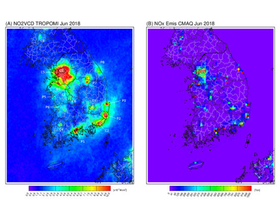
The current South Korean emission inventory, CAPSS 2016, represents the geographical distributions of the NOx emission sources over the country well. It shows good agreement (e.g., R = 0.96 for June 2018) with the TROPOMI NO2 column density distribution;
(2)
The model biases compared with the satellite and surface observations are generally consistent in their spatial patterns, showing overestimations over the SMA and major point sources and underestimations in other locations;
(3)
The modeled column densities overestimate all year, whereas the modeled surface concentrations mostly underestimate, especially during the cold season;
(4)
The diurnal variation agrees better in urban monitoring sites than in roadside monitoring sites. Prominent underestimations of daytime concentrations at roadside monitors are observed;
(5)
The modeled NO2:NOx ratio is higher than that of observations in all cases, and the largest differences are observed at roadside sites.
From these findings, we conclude that most power plants and industrial facilities were well detected by TROPOMI, implying that it can play a critical role in monitoring emission sources in urban areas. We also confirm that the spatial distribution of TROPOMI is consistent with the surface observations, suggesting that the newly available TROPOMI data can be a useful tool for monitoring fine-scale emission sources. TROPOMI has excellent spatial resolution, and it resolves and detects signals from known point sources in South Korea. We also find that the model usually overestimates both columnar and surface NO2 concentrations over the SMA and major point sources, especially during the warm season. One notable exception is the underestimation for cement industries, implying that further investigations are required for emissions from those facilities.
While the interpretation of the model comparison is used to evaluate emission inventories, the comparisons shown in this study suggest a complicated interpretation to decide if the CAPSS 2016 NOx emission inventory is accurately estimated. Using such a simple comparison, both NO and NO2 concentrations are widely underestimated in CAPSS 2016. However, the model overestimates compared with the surface observations in a large number of sites. The key point is that those sites are near the core of strong NOx emission sources, at the center of the SMA and in major industrial point sources. Hence, this mixed result from the NOx concentration comparison fails to provide clear evidence of a NOx emission underestimation or overestimation. It might thus be a premature conclusion to directly link the overestimation of the concentration to the overestimation of emissions, and uncertainty due to the model’s limitations should be considered when interpreting the results of our study.

Supplementary Materials

The following are available online at https://www.mdpi.com/2073-4433/11/1/101/s1. Figure S1: Model performance evaluations for PM2.5, O3 and NO2 concentration over South Korea. Black circles indicate surface observations, and blue lines indicate modeled concentrations; Figure S2: NO2 column density distributions of TROPOMI, CMAQ and model biases (CMAQ-TROPOMI); Figure S3: Comparisons of surface and columnar NO2 concentration during May-December 2018; Figure S4: Comparison of modeled and observed surface NO2 concentration during January to March, April to June, July to September, and October to December, 2018; Figure S5:Comparison of modeled and observed surface NO concentration during January to March, April to June, July to September, and October to December, 2018; Figure S6: Zoom-in of major points sources in Figure 7. Numbers indices point source IDs used in Figure 7; Figure S7: Seasonal variation of NO concentrations from AirKorea surface monitoring sites and CMAQ simulations; Figure S8: Diurnal variations of NO concentrations over urban, roadside and rural sites.

Author Contributions

Conceptualization, H.C.K.; methodology, H.C.K., S.K., and B.-U.K.; formal analysis, H.C.K.; writing—original draft preparation, H.C.K.; writing—review and editing, S.-H.L., B.-U.K. and P.L.; visualization, H.C.K.; funding acquisition, S.K. All authors have read and agreed to the published version of the manuscript.

Acknowledgments

The study was supported by the National Strategic Project-Fine Particle of the National Research Foundation of Korea (NRF) funded by the Ministry of Science and ICT (MSIT), the Ministry of Environment (ME) and the Ministry of Health and Welfare (MOHW) (2017M3D8A1092015), in South Korea.

Conflicts of Interest

The authors declare no conflict of interest.

References

  1. Georgoulias, A.K.; van der A, R.J.; Stammes, P.; Boersma, K.F.; Eskes, H.J. Trends and trend reversal detection in 2 decades of tropospheric NO2 satellite observations. Atmos. Chem. Phys. 2019, 19, 6269–6294. [Google Scholar] [CrossRef] [Green Version]
  2. Martin, R.V. Global inventory of nitrogen oxide emissions constrained by space-based observations of NO2 columns. J. Geophys. Res. 2003, 108, 4537. [Google Scholar] [CrossRef] [Green Version]
  3. Boersma, K.F.; Eskes, H.J.; Richter, A.; De Smedt, I.; Lorente, A.; Beirle, S.; van Geffen, J.H.G.M.; Zara, M.; Peters, E.; Van Roozendael, M.; et al. Improving algorithms and uncertainty estimates for satellite NO2 retrievals: results from the quality assurance for the essential climate variables (QA4ECV) project. Atmos. Meas. Tech. 2018, 11, 6651–6678. [Google Scholar] [CrossRef] [Green Version]
  4. Beirle, S.; Boersma, K.F.; Platt, U.; Lawrence, M.G.; Wagner, T. Megacity Emissions and Lifetimes of Nitrogen Oxides Probed from Space. Science 2011, 333, 1737–1739. [Google Scholar] [CrossRef]
  5. Leue, C.; Wenig, M.; Wagner, T.; Klimm, O.; Platt, U.; Jähne, B. Quantitative analysis of NOx emissions from Global Ozone Monitoring Experiment satellite image sequences. J. Geophys. Res. Atmos. 2001, 106, 5493–5505. [Google Scholar] [CrossRef] [Green Version]
  6. Pan, L.; Tong, D.; Lee, P.; Kim, H.-C.; Chai, T. Assessment of NOx and O3 forecasting performances in the U.S. National Air Quality Forecasting Capability before and after the 2012 major emissions updates. Atmos. Environ. 2014, 95, 610–619. [Google Scholar] [CrossRef]
  7. Chai, T.; Kim, H.-C.; Lee, P.; Tong, D.; Pan, L.; Tang, Y.; Huang, J.; McQueen, J.; Tsidulko, M.; Stajner, I. Evaluation of the United States National Air Quality Forecast Capability experimental real-time predictions in 2010 using Air Quality System ozone and NO2 measurements. Geosci. Model Dev. 2013, 6, 1831–1850. [Google Scholar] [CrossRef] [Green Version]
  8. Boersma, K.F.; Jacob, D.J.; Bucsela, E.J.; Perring, A.E.; Dirksen, R.; van der A, R.J.; Yantosca, R.M.; Park, R.J.; Wenig, M.O.; Bertram, T.H. Validation of OMI tropospheric NO2 observations during INTEX-B and application to constrain NOx emissions over the eastern United States and Mexico. Atmos. Environ. 2008, 42, 4480–4497. [Google Scholar] [CrossRef] [Green Version]
  9. Tong, D.Q.; Lamsal, L.; Pan, L.; Ding, C.; Kim, H.; Lee, P.; Chai, T.; Pickering, K.E.; Stajner, I. Long-term NOx trends over large cities in the United States during the great recession: Comparison of satellite retrievals, ground observations, and emission inventories. Atmos. Environ. 2015, 107, 70–84. [Google Scholar] [CrossRef]
  10. Tong, D.; Pan, L.; Chen, W.; Lamsal, L.; Lee, P.; Tang, Y.; Kim, H.; Kondragunta, S.; Stajner, I. Impact of the 2008 Global Recession on air quality over the United States: Implications for surface ozone levels from changes in NOx emissions. Geophys. Res. Lett. 2016, 43, 9280–9288. [Google Scholar] [CrossRef] [Green Version]
  11. Duncan, B.N.; Yoshida, Y.; de Foy, B.; Lamsal, L.N.; Streets, D.G.; Lu, Z.; Pickering, K.E.; Krotkov, N.A. The observed response of Ozone Monitoring Instrument (OMI) NO2 columns to NOx emission controls on power plants in the United States: 2005–2011. Atmos. Environ. 2013, 81, 102–111. [Google Scholar] [CrossRef] [Green Version]
  12. Visser, A.J.; Boersma, K.F.; Ganzeveld, L.N.; Krol, M.C. European NOx emissions in WRF-Chem derived from OMI: impacts on summertime surface ozone. Atmos. Chem. Phys. 2019, 19, 11821–11841. [Google Scholar] [CrossRef] [Green Version]
  13. Huijnen, V.; Eskes, H.J.; Poupkou, A.; Elbern, H.; Boersma, K.F.; Foret, G.; Sofiev, M.; Valdebenito, A.; Flemming, J.; Stein, O.; et al. Comparison of OMI NO2 tropospheric columns with an ensemble of global and European regional air quality models. Atmos. Chem. Phys. 2010, 10, 3273–3296. [Google Scholar] [CrossRef] [Green Version]
  14. Curier, R.L.; Kranenburg, R.; Segers, A.J.S.; Timmermans, R.M.A.; Schaap, M. Synergistic use of OMI NO2 tropospheric columns and LOTOS–EUROS to evaluate the NOx emission trends across Europe. Remote Sens. Environ. 2014, 149, 58–69. [Google Scholar] [CrossRef]
  15. De Foy, B.; Wilkins, J.L.; Lu, Z.; Streets, D.G.; Duncan, B.N. Model evaluation of methods for estimating surface emissions and chemical lifetimes from satellite data. Atmos. Environ. 2014, 98, 66–77. [Google Scholar] [CrossRef]
  16. Liu, F.; Beirle, S.; Zhang, Q.; Dörner, S.; He, K.; Wagner, T. NOx lifetimes and emissions of cities and power plants in polluted background estimated by satellite observations. Atmos. Chem. Phys. 2016, 16, 5283–5298. [Google Scholar] [CrossRef] [Green Version]
  17. Liu, F.; Beirle, S.; Zhang, Q.; van der A, R.J.; Zheng, B.; Tong, D.; He, K. NOx emission trends over Chinese cities estimated from OMI observations during 2005 to 2015. Atmos. Chem. Phys. 2017, 17, 9261–9275. [Google Scholar] [CrossRef] [Green Version]
  18. Miyazaki, K.; Sekiya, T.; Fu, D.; Bowman, K.W.; Kulawik, S.S.; Sudo, K.; Walker, T.; Kanaya, Y.; Takigawa, M.; Ogochi, K.; et al. Balance of Emission and Dynamical Controls on Ozone During the Korea-United States Air Quality Campaign From Multiconstituent Satellite Data Assimilation. J. Geophys. Res. Atmos. 2019, 124, 387–413. [Google Scholar] [CrossRef] [Green Version]
  19. Mijling, B.; van der A, R.J.; Zhang, Q. Regional nitrogen oxides emission trends in East Asia observed from space. Atmos. Chem. Phys. 2013, 13, 12003–12012. [Google Scholar] [CrossRef] [Green Version]
  20. Zhang, L.; Lee, C.S.; Zhang, R.; Chen, L. Spatial and temporal evaluation of long term trend (2005–2014) of OMI retrieved NO2 and SO2 concentrations in Henan Province, China. Atmos. Environ. 2017, 154, 151–166. [Google Scholar] [CrossRef]
  21. Mijling, B.; van der A, R.J. Using daily satellite observations to estimate emissions of short-lived air pollutants on a mesoscopic scale. J. Geophys. Res. Atmos. 2012, 117. [Google Scholar] [CrossRef]
  22. Liu, F.; van der A, R.J.; Eskes, H.; Ding, J.; Mijling, B. Evaluation of modeling NO2 concentrations driven by satellite-derived and bottom-up emission inventories using in situ measurements over China. Atmos. Chem. Phys. 2018, 18, 4171–4186. [Google Scholar] [CrossRef] [Green Version]
  23. Li, M.; Klimont, Z.; Zhang, Q.; Martin, R.V.; Zheng, B.; Heyes, C.; Cofala, J.; Zhang, Y.; He, K. Comparison and evaluation of anthropogenic emissions of SO2 and NOx over China. Atmos. Chem. Phys. 2018, 18, 3433–3456. [Google Scholar] [CrossRef] [Green Version]
  24. Qu, Z.; Henze, D.K.; Capps, S.L.; Wang, Y.; Xu, X.; Wang, J.; Keller, M. Monthly top-down NOx emissions for China (2005–2012): A hybrid inversion method and trend analysis. J. Geophys. Res. Atmos. 2017, 122, 4600–4625. [Google Scholar] [CrossRef]
  25. Lamsal, L.N.; Duncan, B.N.; Yoshida, Y.; Krotkov, N.A.; Pickering, K.E.; Streets, D.G.; Lu, Z.U.S. NO2 trends (2005–2013): EPA Air Quality System (AQS) data versus improved observations from the Ozone Monitoring Instrument (OMI). Atmos. Environ. 2015, 110, 130–143. [Google Scholar] [CrossRef]
  26. Griffin, D.; Zhao, X.; McLinden, C.A.; Boersma, F.; Bourassa, A.; Dammers, E.; Degenstein, D.; Eskes, H.; Fehr, L.; Fioletov, V.; et al. High-Resolution Mapping of Nitrogen Dioxide With TROPOMI: First Results and Validation Over the Canadian Oil Sands. Geophys. Res. Lett. 2019, 46, 1049–1060. [Google Scholar] [CrossRef] [Green Version]
  27. Zheng, Z.; Yang, Z.; Wu, Z. Marinello Spatial Variation of NO2 and Its Impact Factors in China: An Application of Sentinel-5P Products. Remote Sens. 2019, 11, 1939. [Google Scholar] [CrossRef] [Green Version]
  28. Bae, C.; Kim, H.C.; Kim, B.-U.; Kim, S. Surface ozone response to satellite-constrained NOx emission adjustments and its implications. Environ. Pollut. 2019, 113469. [Google Scholar] [CrossRef]
  29. Kim, H.C.; Kwon, S.; Kim, B.-U.; Kim, S. Review of Shandong Peninsular Emissions Change and South Korean Air Quality. J. Korean Soc. Atmos. Environ. 2018, 34, 356–365. [Google Scholar] [CrossRef]
  30. Kim, B.-U.; Bae, C.; Kim, H.C.; Kim, E.; Kim, S. Spatially and chemically resolved source apportionment analysis: Case study of high particulate matter event. Atmos. Environ. 2017, 162, 55–70. [Google Scholar] [CrossRef]
  31. Han, K.M.; Lee, S.; Chang, L.S.; Song, C.H. A comparison study between CMAQ-simulated and OMI-retrieved NO2 columns over East Asia for evaluation of NOx emission fluxes of INTEX-B, CAPSS, and REAS inventories. Atmos. Chem. Phys. 2015, 15, 1913–1938. [Google Scholar] [CrossRef] [Green Version]
  32. Han, K.M.; Lee, C.K.; Lee, J.; Kim, J.; Song, C.H. A comparison study between model-predicted and OMI-retrieved tropospheric NO2 columns over the Korean peninsula. Atmos. Environ. 2011, 45, 2962–2971. [Google Scholar] [CrossRef]
  33. Kim, N.K.; Kim, Y.P.; Morino, Y.; Kurokawa, J.; Ohara, T. Verification of NOx emission inventory over South Korea using sectoral activity data and satellite observation of NO2 vertical column densities. Atmos. Environ. 2013, 77, 496–508. [Google Scholar] [CrossRef]
  34. Lee, J.-H.; Lee, S.-H.; Kim, H.C. Detection of Strong NOx Emissions from Fine-scale Reconstruction of the OMI Tropospheric NO2 Product. Remote Sens. 2019, 11, 1861. [Google Scholar] [CrossRef] [Green Version]
  35. Goldberg, D.L.; Saide, P.E.; Lamsal, L.N.; de Foy, B.; Lu, Z.; Woo, J.-H.; Kim, Y.; Kim, J.; Gao, M.; Carmichael, G.; et al. A top-down assessment using OMI NO2 suggests an underestimate in the NOx emissions inventory in Seoul, South Korea, during KORUS-AQ. Atmos. Chem. Phys. 2019, 19, 1801–1818. [Google Scholar] [CrossRef] [Green Version]
  36. Choi, M.W.; Lee, J.H.; Woo, J.W.; Kim, C.H.; Lee, S.H. Comparison of PM2.5 Chemical Components over East Asia Simulated by the WRF-Chem and WRF/CMAQ Models: On the Models’ Prediction Inconsistency. Atmosphere 2019, 10, 618. [Google Scholar] [CrossRef] [Green Version]
  37. Nguyen, H.T.; Kim, K.-H.; Park, C. Long-term trend of NO2 in major urban areas of Korea and possible consequences for health. Atmos. Environ. 2015, 106, 347–357. [Google Scholar] [CrossRef]
  38. Irie, H.; Muto, T.; Itahashi, S.; Kurokawa, J.; Uno, I. Turnaround of Tropospheric Nitrogen Dioxide Pollution Trends in China, Japan, and South Korea. Sola 2016, 12, 170–174. [Google Scholar] [CrossRef] [Green Version]
  39. Shon, Z.-H.; Kim, K.-H. Impact of emission control strategy on NO2 in urban areas of Korea. Atmos. Environ. 2011, 45, 808–812. [Google Scholar] [CrossRef]
  40. Kim, S.; Jeong, D.; Sanchez, D.; Wang, M.; Seco, R.; Blake, D.; Meinardi, S.; Barletta, B.; Hughes, S.; Jung, J.; et al. The Controlling Factors of Photochemical Ozone Production in Seoul, South Korea. Aerosol Air Qual. Res. 2018, 18, 2253–2261. [Google Scholar] [CrossRef]
  41. Lee, D.; Lee, Y.-M.; Jang, K.-W.; Yoo, C.; Kang, K.-H.; Lee, J.-H.; Jung, S.-W.; Park, J.-M.; Lee, S.-B.; Han, J.-S.; et al. Korean National Emissions Inventory System and 2007 Air Pollutant Emissions. Asian J. Atmos. Environ. 2011, 5, 278–291. [Google Scholar] [CrossRef] [Green Version]
  42. Elizabeth, C.E. Technical Assistance Document for the Chemiluminescence Measurement of Nitrogen Dioxide. EPA, 1975. Available online: https://www3.epa.gov/ttnamti1/archive/files/ambient/criteria/reldocs/4-75-003.pdf (accessed on 10 January 2020).
  43. Steinbacher, M.; Zellweger, C.; Schwarzenbach, B.; Bugmann, S.; Buchmann, B.; Ordóñez, C.; Prevot, A.S.H.; Hueglin, C. Nitrogen oxide measurements at rural sites in Switzerland: Bias of conventional measurement techniques. J. Geophys. Res. 2007, 112, D11307. [Google Scholar] [CrossRef] [Green Version]
  44. Van Geffen, J.H.G.M.; Eskes, H.J.; Boersma, K.F.; Maasakkers, J.D.; Veefkind, J.P. TROPOMI ATBD of the total and Tropospheric NO2 Data Products. Ministry of Infrastructure and Water Management, 2019. Available online: https://sentinel.esa.int/documents/247904/2476257/Sentinel-5P-TROPOMI-ATBD-NO2-data-products (accessed on 10 January 2020).
  45. Eskes, H.; van Geffen, J.; Boersma, K.F.; Eichmann, K.-U.; Apituley, A.; Pedergnana, M.; Sneep, M.; Veefkind, P.J.; Loyola, D. Sentinel-5 precursor/TROPOMI Level 2 Product User Manual Nitrogen Dioxide. Ministry of Infrastructure and Water Management, 2019. Available online: https://sentinel.esa.int/documents/247904/2474726/Sentinel-5P-Level-2-Product-User-Manual-Nitrogen-Dioxide (accessed on 10 January 2020).
  46. Skamarock, W.C.; Klemp, J.B. A time-split nonhydrostatic atmospheric model for weather research and forecasting applications. J. Comput. Phys. 2008, 227, 3465–3485. [Google Scholar] [CrossRef]
  47. Byun, D.; Schere, K.L. Review of the Governing Equations, Computational Algorithms, and Other Components of the Models-3 Community Multiscale Air Quality (CMAQ) Modeling System. Appl. Mech. Rev. 2006, 59, 51. [Google Scholar] [CrossRef]
  48. Otte, T.L.; Pleim, J.E. The Meteorology-Chemistry Interface Processor (MCIP) for the CMAQ modeling system: updates through MCIPv3.4.1. Geosci. Model Dev. 2010, 3, 243–256. [Google Scholar] [CrossRef] [Green Version]
  49. Carter, W.P.L. The SAPRC-99 Chemical Mechanism and Updated VOC Reactivity Scales. University of California Riverside, 2003. Available online: http://www.cert.ucr.edu/~carter/reactdat.htm (accessed on 10 January 2020).
  50. Jang, Y.; Lee, Y.; Kim, J.; Kim, Y.; Woo, J.-H. Improvement China Point Source for Improving Bottom-Up Emission Inventory. Asia-Pac. J. Atmos. Sci. 2019, 1–12. [Google Scholar] [CrossRef]
  51. Guenther, A.; Karl, T.; Harley, P.; Wiedinmyer, C.; Palmer, P.I.; Geron, C. Estimates of global terrestrial isoprene emissions using MEGAN (Model of Emissions of Gases and Aerosols from Nature). Atmos. Chem. Phys. 2006, 6, 3181–3210. [Google Scholar] [CrossRef] [Green Version]
  52. NCEP NCEP FNL Operational Model Global Tropospheric Analyses, Continuing From July 1999; Research Data Archive, Computational and Information Systems Laboratory: Boulder, CO, USA, 2000; Available online: https://doi.org/10.5065/D6M043C6 (accessed on 10 January 2020).
  53. Hong, S.-Y.; Dudhia, J.; Chen, S.-H. A Revised Approach to Ice Microphysical Processes for the Bulk Parameterization of Clouds and Precipitation. Mon. Weather Rev. 2004, 132, 103–120. [Google Scholar] [CrossRef]
  54. Kain, J.S. The Kain–Fritsch Convective Parameterization: An Update. J. Appl. Meteorol. 2004, 43, 170–181. [Google Scholar] [CrossRef] [Green Version]
  55. Chen, F.; Dudhia, J. Coupling an Advanced Land Surface–Hydrology Model with the Penn State–NCAR MM5 Modeling System. Part I: Model Implementation and Sensitivity. Mon. Weather Rev. 2001, 129, 569–585. [Google Scholar] [CrossRef] [Green Version]
  56. Hong, S.-Y.; Noh, Y.; Dudhia, J. A new vertical diffusion package with an explicit treatment of entrainment processes. Mon. Weather Rev. 2006, 134, 2318–2341. [Google Scholar] [CrossRef] [Green Version]
  57. Hertel, O.; Berkowicz, R.; Christensen, J.; Hov, Ø. Test of two numerical schemes for use in atmospheric transport-chemistry models. Atmos. Environ. Part A. Gen. Top. 1993, 27, 2591–2611. [Google Scholar] [CrossRef]
  58. Binkowski, F.S. Models-3 Community Multiscale Air Quality (CMAQ) model aerosol component 1. Model description. J. Geophys. Res. 2003, 108, 4183. [Google Scholar] [CrossRef]
  59. Yamartino, R.J. Nonnegative, Conserved Scalar Transport Using Grid-Cell-centered, Spectrally Constrained Blackman Cubics for Applications on a Variable-Thickness Mesh. Mon. Weather Rev. 1993, 121, 753–763. [Google Scholar] [CrossRef] [Green Version]
  60. Louis, J.-F. A parametric model of vertical eddy fluxes in the atmosphere. Bound-Lay. Meteorol. 1979, 17, 187–202. [Google Scholar] [CrossRef]
  61. Chang, J.S.; Brost, R.A.; Isaksen, I.S.A.; Madronich, S.; Middleton, P.; Stockwell, W.R.; Walcek, C.J. A three-dimensional Eulerian acid deposition model: Physical concepts and formulation. J. Geophys. Res. 1987, 92, 14681. [Google Scholar] [CrossRef]
  62. Kim, H.C.; Lee, P.; Judd, L.; Pan, L.; Lefer, B. OMI NO2 column densities over North American urban cities: the effect of satellite footprint resolution. Geosci. Model Dev. 2016, 9, 1111–1123. [Google Scholar] [CrossRef] [Green Version]
  63. Kim, H.; Lee, S.-M.; Chai, T.; Ngan, F.; Pan, L.; Lee, P. A Conservative Downscaling of Satellite-Detected Chemical Compositions: NO2 Column Densities of OMI, GOME-2, and CMAQ. Remote Sens. 2018, 10, 1001. [Google Scholar] [CrossRef] [Green Version]
  64. Valin, L.C.; Russell, A.R.; Hudman, R.C.; Cohen, R.C. Effects of model resolution on the interpretation of satellite NO2 observations. Atmos. Chem. Phys. 2011, 11, 11647–11655. [Google Scholar] [CrossRef] [Green Version]
  65. De Foy, B.; Krotkov, N.A.; Bei, N.; Herndon, S.C.; Huey, L.G.; Martínez, A.-P.; Ruiz-Suárez, L.G.; Wood, E.C.; Zavala, M.; Molina, L.T. Hit from both sides: tracking industrial and volcanic plumes in Mexico City with surface measurements and OMI SO2 retrievals during the MILAGRO field campaign. Atmos. Chem. Phys. 2009, 9, 9599–9617. [Google Scholar] [CrossRef] [Green Version]
  66. Russell, A.R.; Valin, L.C.; Bucsela, E.J.; Wenig, M.O.; Cohen, R.C. Space-based Constraints on Spatial and Temporal Patterns of NOx Emissions in California, 2005−2008. Environ. Sci. Technol. 2010, 44, 3608–3615. [Google Scholar] [CrossRef] [PubMed]
  67. Mavroidis, I.; Chaloulakou, A. Long-term trends of primary and secondary NO2 production in the Athens area. Variation of the NO2/NOx ratio. Atmos. Environ. 2011, 45, 6872–6879. [Google Scholar] [CrossRef]
  68. Wild, R.J.; Dubé, W.P.; Aikin, K.C.; Eilerman, S.J.; Neuman, J.A.; Peischl, J.; Ryerson, T.B.; Brown, S.S. On-road measurements of vehicle NO2 /NOx emission ratios in Denver, Colorado, USA. Atmos. Environ. 2017, 148, 182–189. [Google Scholar] [CrossRef]
  69. Costantini, M.G.; Khalek, I.; McDonald, J.D.; van Erp, A.M. The Advanced Collaborative Emissions Study (ACES) of 2007- and 2010-Emissions Compliant Heavy-Duty Diesel Engines: Characterization of Emissions and Health Effects. Emiss. Control Sci. Technol. 2016, 2, 215–227. [Google Scholar] [CrossRef] [Green Version]
  70. May, A.A.; Nguyen, N.T.; Presto, A.A.; Gordon, T.D.; Lipsky, E.M.; Karve, M.; Gutierrez, A.; Robertson, W.H.; Zhang, M.; Brandow, C.; et al. Gas- and particle-phase primary emissions from in-use, on-road gasoline and diesel vehicles. Atmos. Environ. 2014, 88, 247–260. [Google Scholar] [CrossRef]
  71. Richmond-Bryant, J.; Chris Owen, R.; Graham, S.; Snyder, M.; McDow, S.; Oakes, M.; Kimbrough, S. Estimation of on-road NO2 concentrations, NO2/NOX ratios, and related roadway gradients from near-road monitoring data. Air Qual. Atmos. Heal. 2017, 10, 611–625. [Google Scholar] [CrossRef]
  72. Kimbrough, S.; Chris Owen, R.; Snyder, M.; Richmond-Bryant, J. NO to NO2 conversion rate analysis and implications for dispersion model chemistry methods using Las Vegas, Nevada near-road field measurements. Atmos. Environ. 2017, 165, 23–34. [Google Scholar] [CrossRef]
  73. Kim, Y.P.; Lee, G. Trend of Air Quality in Seoul: Policy and Science. Aerosol. Air Qual. Res. 2018, 18, 2141–2156. [Google Scholar] [CrossRef] [Green Version]
  74. Dickerson, R.R.; Anderson, D.C.; Ren, X. On the use of data from commercial NOx analyzers for air pollution studies. Atmos. Environ. 2019, 214, 116873. [Google Scholar] [CrossRef]
  75. Goldberg, D.L.; Lu, Z.; Streets, D.G.; de Foy, B.; Griffin, D.; McLinden, C.A.; Lamsal, L.N.; Krotkov, N.A.; Eskes, H. Enhanced Capabilities of TROPOMI NO2: Estimating NOX from North American Cities and Power Plants. Environ. Sci. Technol. 2019, 53, 12594–12601. [Google Scholar] [CrossRef]
  76. Anderson, D.C.; Loughner, C.P.; Diskin, G.; Weinheimer, A.; Canty, T.P.; Salawitch, R.J.; Worden, H.M.; Fried, A.; Mikoviny, T.; Wisthaler, A.; et al. Measured and modeled CO and NOy in DISCOVER-AQ: An evaluation of emissions and chemistry over the eastern US. Atmos. Environ. 2014, 96, 78–87. [Google Scholar] [CrossRef]
  77. Canty, T.P.; Hembeck, L.; Vinciguerra, T.P.; Anderson, D.C.; Goldberg, D.L.; Carpenter, S.F.; Allen, D.J.; Loughner, C.P.; Salawitch, R.J.; Dickerson, R.R. Ozone and NOx chemistry in the eastern US: evaluation of CMAQ/CB05 with satellite (OMI) data. Atmos. Chem. Phys. 2015, 15, 10965–10982. [Google Scholar] [CrossRef] [Green Version]
  78. Kota, S.H.; Zhang, H.; Chen, G.; Schade, G.W.; Ying, Q. Evaluation of on-road vehicle CO and NOx National Emission Inventories using an urban-scale source-oriented air quality model. Atmos. Environ. 2014, 85, 99–108. [Google Scholar] [CrossRef]
  79. Jiang, Z.; McDonald, B.C.; Worden, H.; Worden, J.R.; Miyazaki, K.; Qu, Z.; Henze, D.K.; Jones, D.B.A.; Arellano, A.F.; Fischer, E.V.; et al. Unexpected slowdown of US pollutant emission reduction in the past decade. Proc. Natl. Acad. Sci. USA 2018, 115, 5099–5104. [Google Scholar] [CrossRef] [PubMed] [Green Version]
  80. Travis, K.R.; Jacob, D.J.; Fisher, J.A.; Kim, P.S.; Marais, E.A.; Zhu, L.; Yu, K.; Miller, C.C.; Yantosca, R.M.; Sulprizio, M.P.; et al. Why do models overestimate surface ozone in the Southeast United States? Atmos. Chem. Phys. 2016, 16, 13561–13577. [Google Scholar] [CrossRef] [Green Version]
Figure 1. Spatial distribution of (A) NO2 vertical column densities from TROPOMI and (B) NOx emissions from CAPSS 2016 during June 2018. TROPOMI level 2 pixels are oversampled onto a 3-km grid using the conservative spatial regridding method and CAPSS NOx emissions are gridded onto a 9-km domain grid.
Atmosphere 11 00101 g001
Figure 2. NO2 vertical column densities from TROPOMI (upper left) and CMAQ (upper right) and their differences (i.e., CMAQ–TROPOMI) (bottom) during June 2018.
Atmosphere 11 00101 g002
Figure 3. Comparison of the modeled and observed surface NO2 concentrations. Monthly averages of (A) surface observations, (B) interpolated concentration using Krig, (C) model biases (CMAQ-OBS) and (D) differences between model and Kriged concentrations (CMAQ–Krig) during June 2018.
Atmosphere 11 00101 g003
Figure 4. Comparisons of the surface and columnar NO2 concentrations. Scatterplots between the surface observations and CMAQ model (left) and column densities from TROPOMI and CMAQ (right) during June 2018 are shown. For a fair comparison, TROPOMI and CMAQ NO2 column density pixels collocated with the surface monitoring sites are selected. Comparisons for other months are available in Figure S3.
Atmosphere 11 00101 g004
Figure 5. Seasonal variation in NO2 concentration from the surface observations and corresponding CMAQ simulations. Daily mean NO2 concentrations over 305 sites are presented. (a). surface observation; (b). corresponding CMAQ simulation.
Atmosphere 11 00101 g005
Figure 6. Diurnal variation in NO2 concentrations from the surface monitoring sites and model.
Atmosphere 11 00101 g006
Figure 7. Spatial distribution of NOx emissions from point sources in CAPSS 2016. Point source NOx emissions in each 9-km modeling cell are summed and grid cells with more than 2000 ton/year are marked with a blue circle. The numbers shown next to each circle are the IDs (in Figure 8), which are sorted by the order of the model biases. Zoom-in plots for congested areas (e.g., Chungnam, Kwangyang and Pohang) are available in the Supplementary Information.
Atmosphere 11 00101 g007
Figure 8. Comparison of TROPOMI and CMAQ NO2 vertical column densities over major point source emission locations. NO2 column densities from CMAQ and TROPOMI (lower) and biases (i.e., CMAQ-TROPOMI) (upper), sorted by bias size, are shown. Point source indices on the x-axis indicate the cells with point sources more than 2,000 ton/year NOx emissions.
Atmosphere 11 00101 g008
Figure 9. Diurnal variation in the NO2:NOx concentration ratios from the observations (circles) and model (red) at urban, roadside and rural monitoring sites during 2018.
Atmosphere 11 00101 g009
Table 1. Model option configurations for the Weather Research and Forecasting (WRF) and community multiscale air quality (CMAQ) simulations.
ModelConfigurationReference
WRF v3.3Initial field
Microphysics
Cumulus scheme
LSM scheme
PBL scheme
FNL [52]
WSM3 [53]
Kain-Fritsch [54]
NOAH [55]
YSU [56]
CMAQ v4.7.1Chemical mechanism
Chemical solver
Aerosol module
Advection scheme
Horizontal diffusion
Vertical diffusion
Cloud scheme
SAPRC99 [49]
EBI [57]
AERO5 [58]
YAMO [59]
Multiscale [60]
Eddy [60]
RADM [61]
Table 2. Amount of nitrogen oxide (NOx) emissions from the major source classification codes in CAPSS 2007, 2010, 2013 and 2016.
Source Classification CodeCAPSS
2007201020132016
Combustion in energy industries156,304153,441177,219145,445
Nonindustrial combustion plants82,39696,48088,76985,824
Combustion in manufacturing industries155,053164,942178,034175,332
Production processes48,72549,02255,15155,932
Road transport495,084382,226335,721452,995
Other mobile sources and machinery237,101208,878246,027309,986
Waste treatment and disposal13,0976,0629,52913,570
Other sources and sinks163158165167
Combustion total393,753414,863444,022406,601
Mobile total732,185591,104581,748762,981
Total1,187,9231,061,2101,090,6141,239,251

