Atmospheric Characterization Based on Relative Humidity Control at Optical Turbulence Generator

Abstract

In atmospheric turbulence, relative humidity has been almost a negligible variable due to its limited effect, compared with temperature and air velocity, among others. For studying the horizontal path, a laser beam was propagated in a laboratory room, and an Optical Turbulence Generator (OTG) was built and placed along the optical axis. Additionally, there was controlled humidity inside the room and measuring of some physical variables inside the OTG device for determining its effects on the laser beam. The experimental results show the measurements of turbulence parameters $C_n^2$, $l_o$, and ${\sigma }_I^2$ from beam centroids fluctuations, where increases in humidity generated stronger turbulence.

1. Introduction

Turbulence theories had helped to study the atmosphere for many years [1,2,3], and different dissertations, research papers, and projects have been proposed [4,5,6,7,8,9,10]. Those works have applied theories to evaluate statistically wavefront distortions and the angle of arrival fluctuations, including an updated study applied in a closed industrial environment, among others. Their main goal was to measure parameters of turbulence employing techniques such as Moiré deflectometry, telescopy, and collimated beams, incorporating some aberrations by collimated and focused processes, which could generate precision issues despite of the good results obtained. However, it is important to highlight that there are techniques to evaluate key parameters, such as inner scale ($l_0$), refraction structure index ($C_n^2$), and arrival angle (α) in the atmosphere propagation beam. Part of those methods was used in this work.

On the other hand, some reports indicate that not only one physical parameter can change turbulence behavior [11], and this fact motivated the construction of an OTG. It was built from a metal pipe, where some experiments to different relative humidity from water vapor were included [12].

Humidity is a measurement that generally refers to the amount of water vapor in the atmosphere. Each atmospheric gas has its own pressure and a specific number of molecules in a given temperature. The saturation vapor pressure is the pressure of vapor when liquid water begins to condense. Thus, relative humidity is determined as the current vapor pressure divided by the saturation vapor pressure [13].

Experiments were conducted with a scheme to study beam wander and atmospheric turbulence [14]. In this scheme, a few optical and electronic elements for measuring changes in the humidity parameter were included. Electronic sensors were previously calibrated to find a relation between relative humidity and beam centroid movements. This was possible with the use of an optical synchronization system that was operated with photodetectors, microcontrollers, and laptop-controlled cameras [12].

Data were processed and analyzed from the acquired images, achieving the assessment of fluctuations and turbulence parameters without using a lens to focus or expanding the beam, thus introducing less aberrations errors. There are some interesting findings that reveal fluctuations in the analysis of the binary effective area once the methods to generate turbulence from humidity are established. Besides, since the current systems employed to measure turbulence parameters are expensive, the model presented for evaluating humidity shows a simple technique that produces good results with less elements. Future works will consider the Fourier Telescopy scheme presented in [15], and the phase analysis [16] of Young’s fringes pattern obtained after the beam horizontal propagation.

2. Proposed System Description and Methods

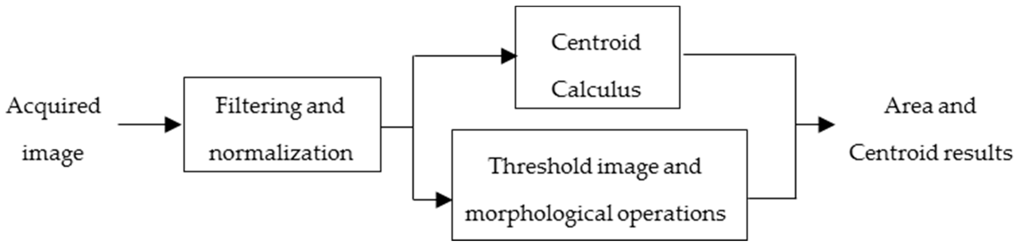
Mathematical methods for studying turbulence parameters in this paper were based on movements of the laser beam spot acquired on CMOS cameras. The gray level centroids were estimated from these digitized images in order to evaluate their temporal fluctuation (as shown in Figure 1).

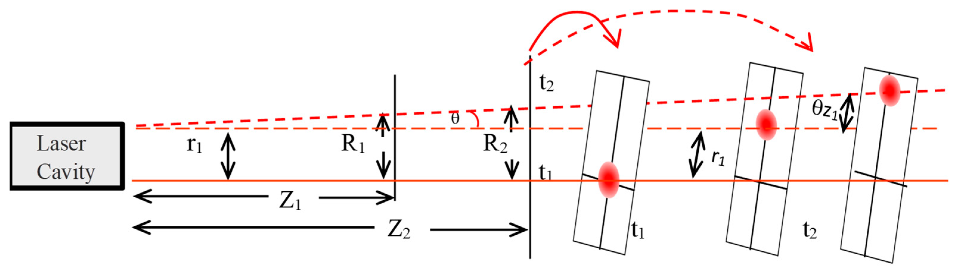
The centroids are included in the model shown in [14], whose purpose is to split laser cavity effects (mainly beam wander) of turbulence effects in the atmosphere. Figure 2 shows a spot on two planes located at distances $z_1$ and $z_2$ from the laser output, and the beam shifting that is modeled by $r_1$ and $\theta$ as translation and tilt, respectively, at times $t_1$ and $t_2$.

From geometric optics, if $z_1$ is longer than the Rayleigh range and $\theta$ is smaller, $z_1$ and $z_2$ distances lead to:

$$R_1=r_1+{\theta z}_1,$$

(1)

$$R_2=r_1+\theta z_2,$$

(2)

where $R_1$ and $R_2$ model the position of the centroids computed from CMOS-1 and CMOS-2 (as shown in Figure 3 below); $r_1$ and $\theta$ are known whether the spot is captured in two different instants ($t_1$ and $t_2$). Notice that the time is discretized in order to find $\theta$ and to estimate the turbulence parameters from the fluctuations of the temporal angle and the scintillation index.

For computing the propagation angle in the Cartesian coordinates from geometric optics, let

$${\theta }_x\left(k\right)=\frac{x_{n2}\left(k\right)-x_{n1}\left(k\right)}{z_2-z_1}$$

(3)

and

$${\theta }_y\left(k\right)=\frac{y_{n2}\left(k\right)-y_{n1}\left(k\right)}{z_2-z_1},$$

(4)

where $n_1$ and $n_2$ refer to two planes at $z_1$ and $z_2$ respectively, and $k$ refers to the iteration time. These equations are used to estimate the location of the beam with only the beam wander effect in a plane at $z_3$ from the laser output. Similarly, the Equations (3) and (4) are computed only in the third plane ($z_3$) and two adjacent times ($k$ and $k+1$) in order to evaluate the spatial fluctuations with regards to the time.

On the other hand, the scintillation index, which measures intensity fluctuations, can be computed as:

$${\sigma }_I^2=\frac{\langle I^2\rangle }{\langle I^2\rangle }-1,$$

(5)

whose expression corresponds to a line-of-sight laser communication link and the inner scale as:

$$l_o=1.08z_3\sqrt{\frac{\langle {\theta }^2\rangle }{{\sigma }_I^2}},$$

(6)

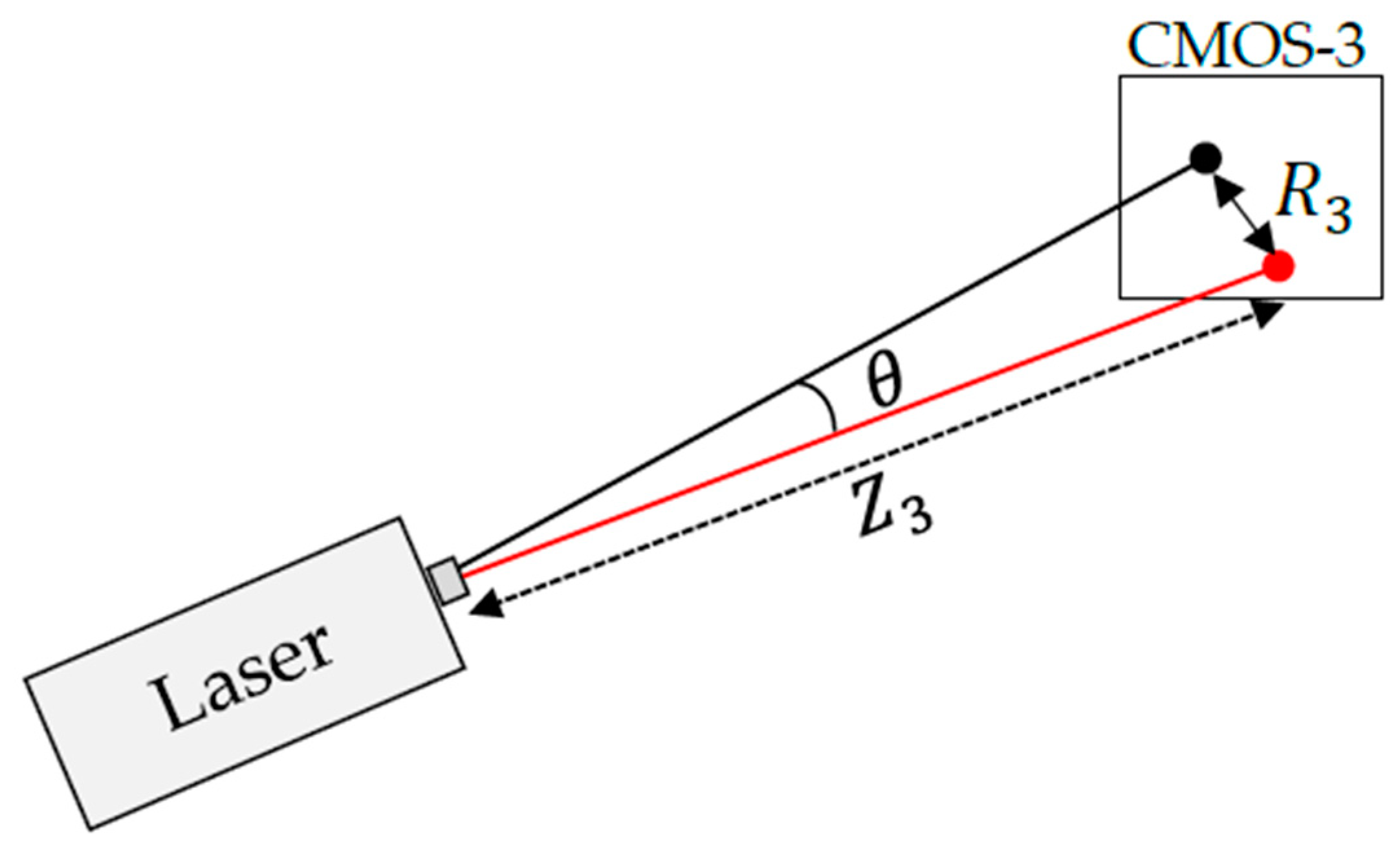
with $z_3$ as the propagation distance, $\theta$ as (3–4), which corresponds to the cylindrical coordinates as depicted in Figure 4. Lastly, the refraction index can be computed from Equation (6) shown in [7] as:

$$C_n^2=\frac{{\sigma }_I^2}{1.23k^{7/6}{z}_3^{11/6}},$$

(7)

where, $k=\frac{2\pi }{\lambda }$ is the wave vector. The parameter $C_n^2$ is important since it characterizes the different stages as summarized in [10]. For example, Davis scale presents $C_n^2~{10}^{-18}{m}^{-2/3}$ as a very weak turbulence, $C_n^2~{10}^{-16}{m}^{-2/3}$ as weak turbulence, and $C_n^2~{10}^{-14}{m}^{-2/3}$ as strong turbulence [17], while Wilfter and Dordowa include two stages: $C_n^2~{10}^{-13}{m}^{-2/3}$ as very strong turbulence and $C_n^2~{10}^{-15}{m}^{-2/3}$ as mean turbulence [18].

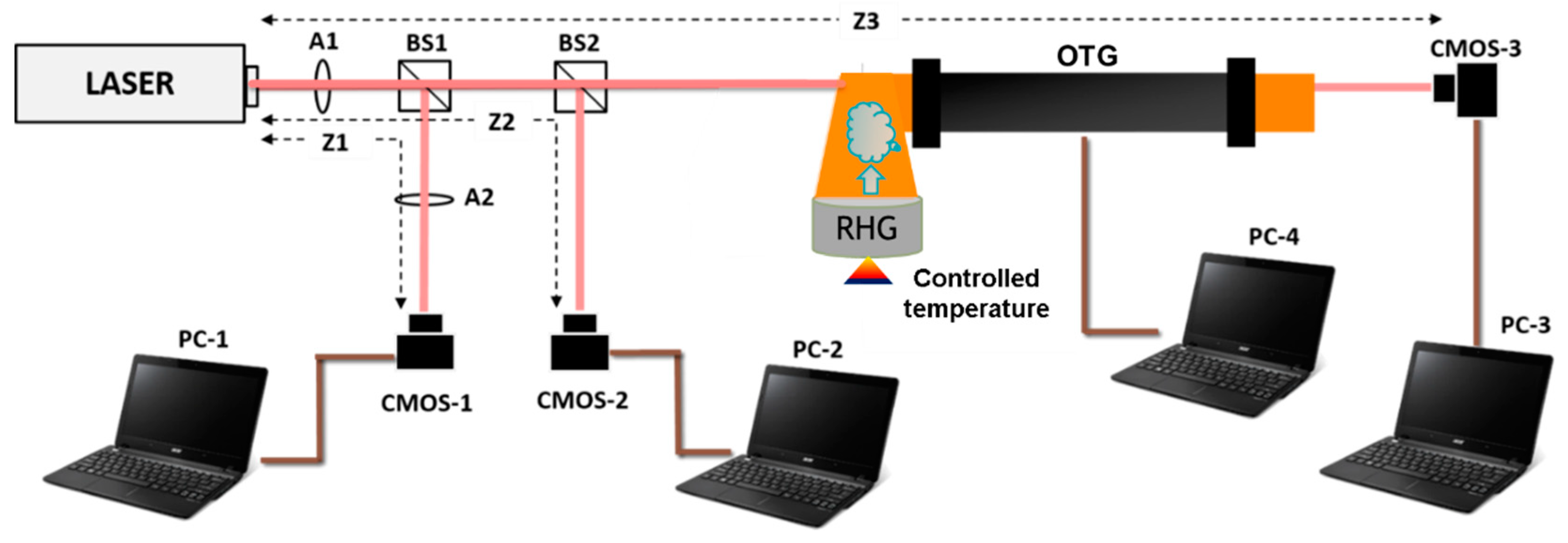
Considering Equations (1)–(7) and the beam wander effects produced by laser cavity, the setup to acquire the information consists of a laser beam that is propagated horizontally, two CMOS sensors for measuring the propagation and position of the laser beam in non-controlled conditions, a relative humidity generator, an OTG (with a relative humidity sensor inside), and another CMOS sensor for measuring the propagation in its XY coordinate plane, perpendicular to the Z axis of the laser beam propagation and after the altered propagation conditions. Figure 3 illustrates the setup configuration, and

Table 1. Summary of the main setup parameters.

Device	Characteristics
Laser	He-Ne Laser. Model 127-35. Power output: 35 mW. Wavelength: 632.8 nm [19].
CMOS Camera	Model: 1312C. Pixel Size: 5.3 μm. Pixels (H × V): 1280 × 1024. Area (H × V) (mm): 6.79 × 5.43 [20].
Relative Humidity Sensor	HST2030SMD – Temperature and Humidity Sensor by Measurement specialties [21]
Laptop	Intel processor, Core i3–i5. RAM Memory: 4GB.
Software	MATLAB ®, Arduino Platform [22], IDS uEye [23].
RHG	Metal pot with an electronic temperature control.

. shows the specifications of its components. The setup is based on the design proposed in Reference [14], but relative humidity is inserted in the OTG by controlling the water temperature inside a pot during the experiments. That is to say, the source of relative humidity is located under the OTG and a plastic pipe located transversally to the laser beam guides it. There is a hole in the left side of the pipe to propagate the laser beam from the OTG to the last sensor. PC-1 to PC-3 control the CMOS cameras acquisition, while PC-4 is used for programming and acquiring the relative humidity sensors data via an Arduino platform. Those sensors are located inside the OTG in three different positions: 10 cm, 60 cm, and 95 cm from its left edge

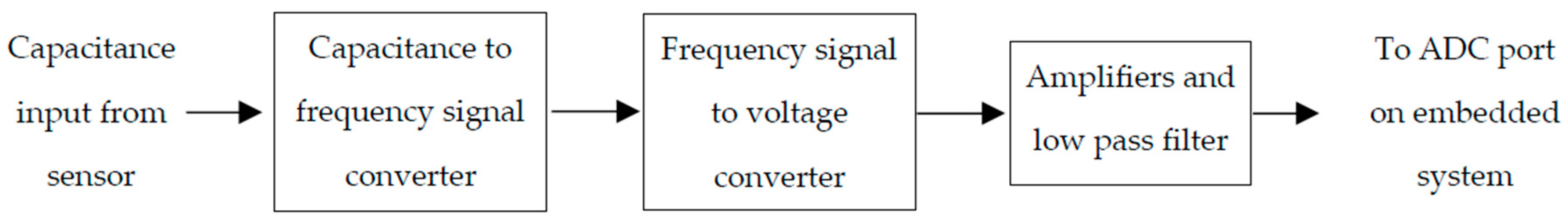
A coupled hardware architecture was designed to measure the humidity, taking advantage of the capacitance variable sensor (Table 1). That variable was used as input of a circuit to generate frequency, so that any change in capacitance is transduced in a change in frequency. Lastly, the output signal transduced to voltage is filtered, amplified, and coupled to a microcontroller (from Analog to Digital Converter—ADC). Figure 5 shows the devices designed and their signal processing scheme is shown in Figure 6.

Data acquisition starts with an optical synchronization, as shown in Figure 3. Cameras and sensors are set up before the laser beam port is opened. Thus, each subsystem is operating in an isolated manner under the frozen turbulence hypothesis [24]. Timers are programmed to acquire 1800 samples at a sampling frequency of 1 Hz. The number of samples considers the evaluation of humidity stability, calculation of the average time in turbulence parameter, and the sampling frequency to warrant synchronized acquisition over all devices (cameras, PCs, and micro-controller).

3. Results

Several experimental scenarios with controlled relative humidity were designed in order to evaluate the effects of relative humidity in the turbulence parameters. Some air temperature measurements are also summarized in

Table 2. Tests designed. Source: Authors.

Test Name	Relative Humidity (RH) Average (%)	RH Standard Deviation (%)	Temperature Average (°C)	T Standard Deviation (°C)
Pattern	64.05	±0.49	30.12	±0.32
Test 1	99.13	±0.26	31.13	±0.20
Test 2	57.88	±1.18	34.23	±0.08
Test 3	84.61	±1.49	29.8	±0.27

however, they were only references because the changes made in humidity lead to few changes in air temperature.

3.1. Synchronization

The synchronization time is measured from the previously programmed timers of MATLAB® and the Arduino Platform.

Table 3. Synchronization time of different tests (Maximum and Minimum time in bold).

Test Name	PC1 vs PC2 (ms)		PC1 vs PC3 (ms)		PC1 vs PC4 (ms)
	Time	Stand. Dev.	Time	Stand. Dev.	Time	Stand. Dev.
Pattern	26,45	16,57	40,3	18,8	13,84	8,10
Test 1	12,16	11,57	19,18	10,69	7,01	7,23
Test 2	39,27	30,61	34,77	19,19	4,49	8,13
Test 3	45,21	20,63	38,05	19,19	7,16	7,85

reports the experimental time for each test listed on Table 2. Notice that the worst case corresponds to Test 3, and the best average synchronization time corresponds to Test 1, following the frozen turbulence hypothesis [24].

After the acquisition, a time model from [14] is implemented. It studies the transversal displacements of laser beam centroids and their 2D distribution; then, each spatial shift between times $k$ and $k+1$ is registered by all CMOS cameras. Therefore, it is used to find the centroid temporal distribution from Equations (1)–(4) of the images acquired by CMOS-1 and CMOS-2 and their estimated centroid at $z_3$ (CMOS-3 in Figure 3), and lastly, the current centroid on the CMOS-3 image.

3.2. Centroids Fluctuations

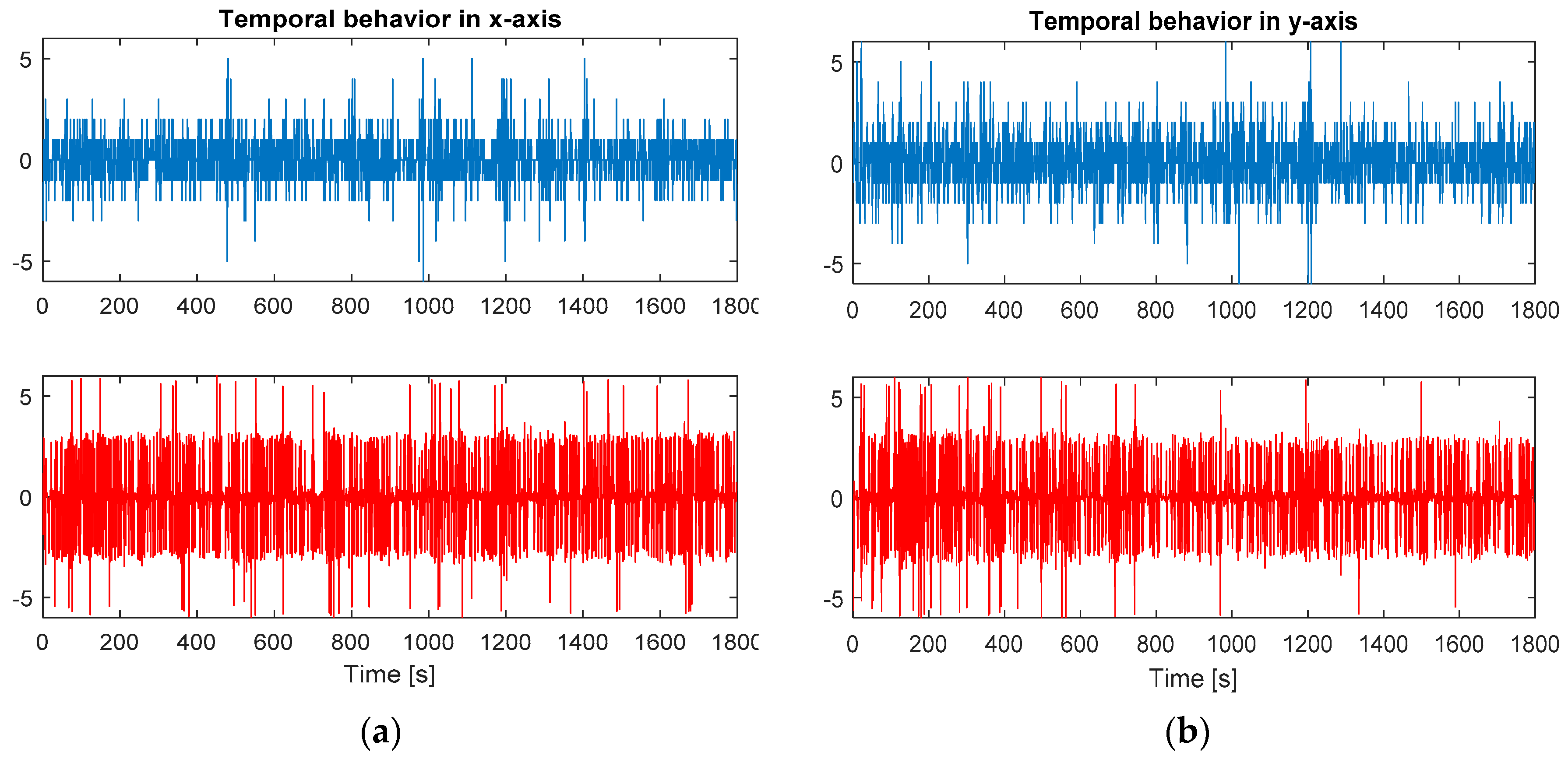
The first temporal fluctuation orders along the x and y-axis are calculated and analyzed from both the measured and estimated centroids (see Figure 7). In this section, movements are modeled as discrete variables; then, the minimum shifting calculated or estimated is a pixel.

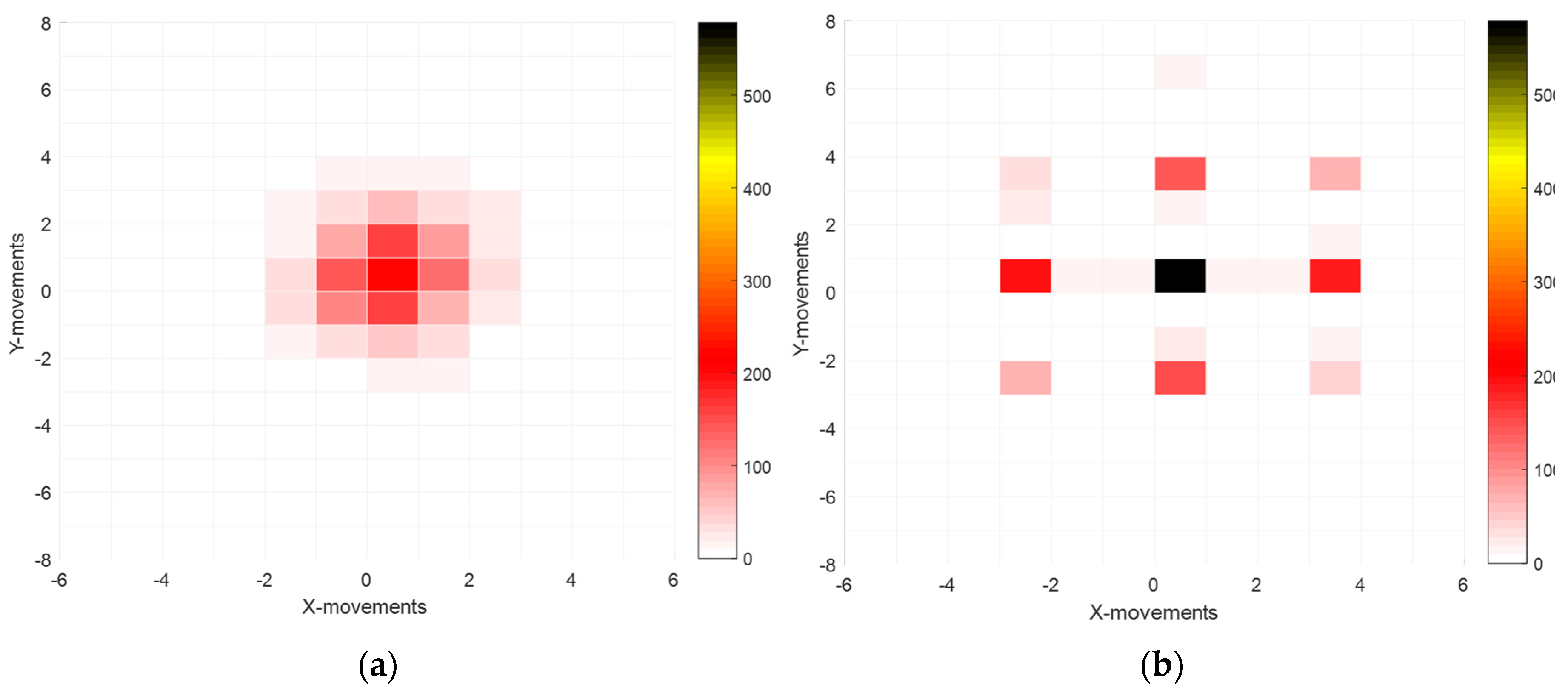
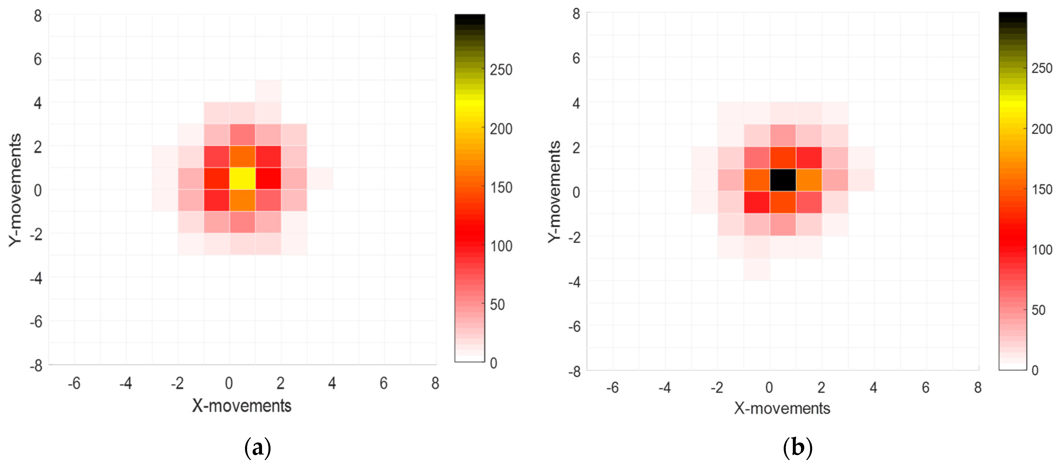
Figure 7 shows how the centroids measurements are near the center value (zero) and in both cases, the maximum fluctuation is close to 6 pixels. The results are similar in the estimated centroids, but there are effects due to the pixel size (see the CMOS Camera on Table 1). These results are shown as a 2D histogram in Figure 8. This representation indicates temporal fluctuations. Notice that the black color on the sidebar corresponds to the highest statistical frequency, while light red corresponds to the lowest frequency. Both the horizontal and vertical axis are movements on the plane of the laser beam centroid.

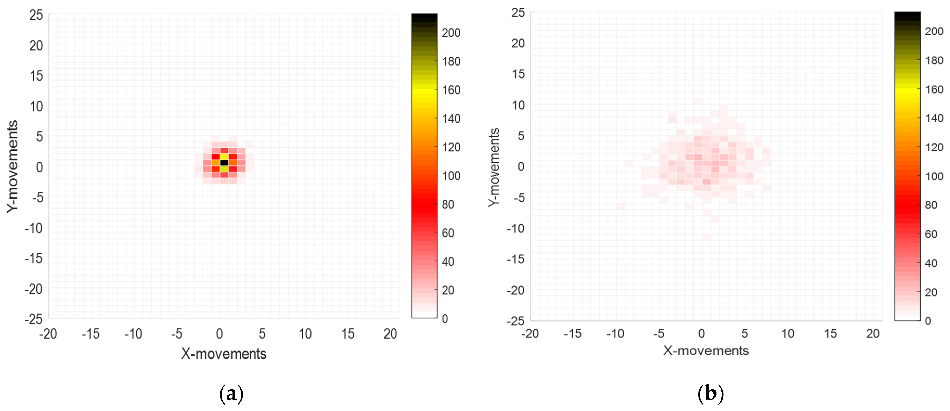
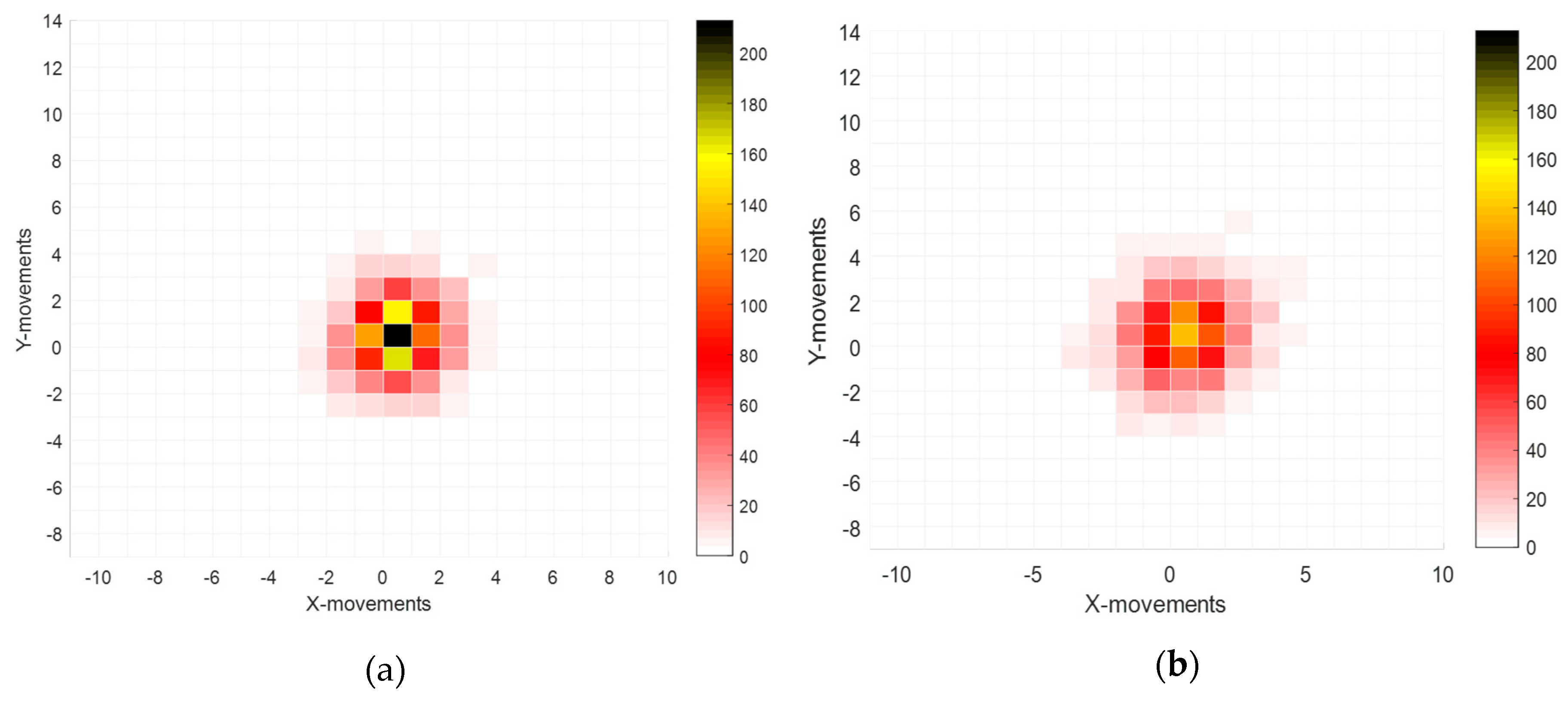
Figure 8 shows the histogram with some null values between pixels close to the center due to $z_3$ propagation distances (this corresponds to the geometrical projection from the plane of cameras CMOS 1-2 to the $z_3$ plane, as shown in Table 1). When the relative humidity is incorporated, their effects over the centroid fluctuations could be measured at $z_3$. Figure 9 shows these compared results.

Notice that the central point (labeled (0,0) corresponding to the optical axis) has the highest frequency in Figure 9a. In contrast, in Figure 9b, the region with the maximal frequency has been shifted several pixels to the right from the central point (which is difficult to see in the linear scale of the color bar), and dispersion of centroid fluctuations changed from ±8 pixels for the Pattern Test to ± 25 pixels for Test #1. Furthermore, results from Test #2 and Test #3 are compared to the Pattern Test, and the results are shown in Figure 10 and Figure 11. In both cases, the dispersion of fluctuations describes the humidity effects in the propagated laser beam. When the dispersion is large, the turbulent effect is strong. It is considered that the experimental setup conditions perhaps generate an additional vortex due to the 90°—incidence angle of the water vapor with regards to the optical path. Then, when the relative humidity produced by the vapor is large, so is the fluctuation of the laser beam centroid.

Notice that the dispersion in Test #2 is lower than in the Pattern Test case. It is caused by the relative humidity. Table 2 shows a relative humidity below the one for the Pattern Test.

3.3. Angle Computation

Results shown in Figure 7 and Equations (1)–(2) are used to measure the $\theta$-angle. Measurements presented in Section 3.2 are proportional to $\theta$, as follows:

$${\theta }_x\left[k\right]=\frac{x\left[k\right]-x\left[k-1\right]}{z_3},{\theta }_y\left[k\right]=\frac{y\left[k\right]-y\left[k-1\right]}{z_3},\theta \left[k\right]=\sqrt{{\theta }_x^2\left[k\right]+{\theta }_y^2\left[k\right]}$$

(8)

The pixel size reported in Table 1 for the CMOS-3 camera is incorporated to convert discrete spatial measurements in the plane into an angular discrete variable. Therefore, each pixel is converted. Figure 12 displays the fluctuations of angle.

These angle fluctuations allow obtaining the angle structure functions and the structure functions for Test #1 to Test #3, which are introduced in the next section.

3.4. Structure Functions and Turbulence Parameters

The structure function from Kolmogorov’s theory [1,25] is used to measure local fluctuations in the centroids and the $\theta$-angle:

$$D_f(\overrightarrow{r})=\langle {[(\overrightarrow{r_1}+\overrightarrow{r})-f(\overrightarrow{r_1})]}^2\rangle ,$$

(9)

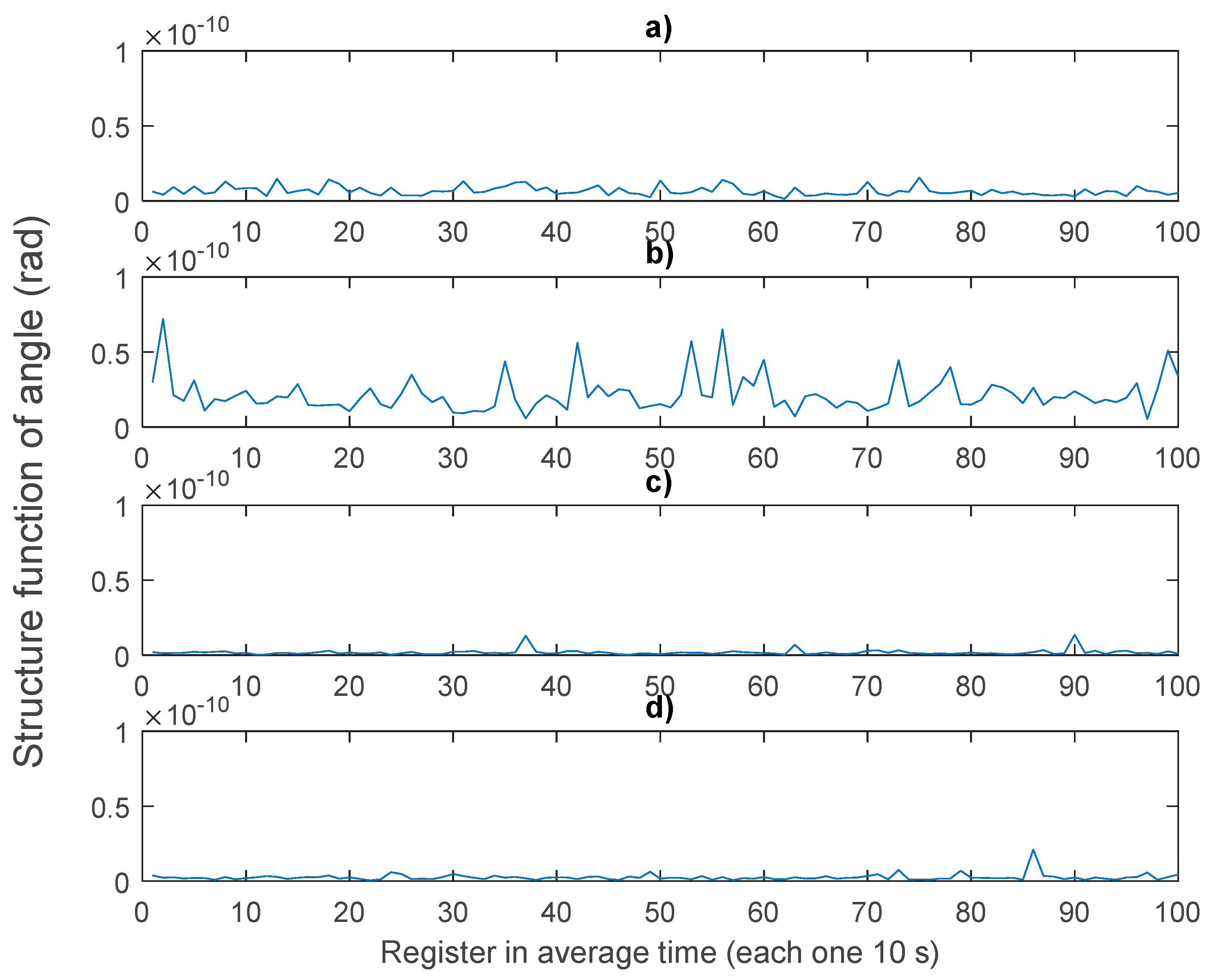
where $D$ is the structure function of $f$, the physical variable; $\overrightarrow{r}$ is a selected position vector to measure $D$; $\overrightarrow{r_1}$ is any other position vector relative and close to $\overrightarrow{r}$, assuming a homogeneous region in the acquisition area (on the CMOS camera plane); and 〈 〉 indicates the average time. After analysis, fluctuations are classified in groups of ten consecutive samples to compute the average time for getting the fluctuation angle of the centroid for each test as shown in Figure 13 (only for the first 1000 samples) and in

Table 4. Statistics of parameters to calculate $\theta$ and ${\sigma }_I^2$.

Test Name	$\mathit{\theta }$ Average Angle (prad)	$\mathit{\theta }$ Stand. Dev. Angle (prad)	${\mathit{\sigma }}_{\mathit{I}}^2$ Average (10−6)	${\mathit{\sigma }}_{\mathit{I}}^2$ Stand. Dev. (10−6)	${\mathit{l}}_0$ Average (mm)	${\mathit{l}}_0$ Stand. Dev. (mm)
Pattern	2.02	2.15	0.58	0.71	16.31	6.98
Test 1	34.8	34.2	243.4	133.1	6.02	4.16
Test 2	2.39	2.66	1.14	2. 08	7.37	4.17
Test3	3.64	5.15	5.89	0.55	6.97	3.70

for all of the samples. Fluctuations are measured in relation to the average value of the angle of centroid ($\overline{\theta }$).

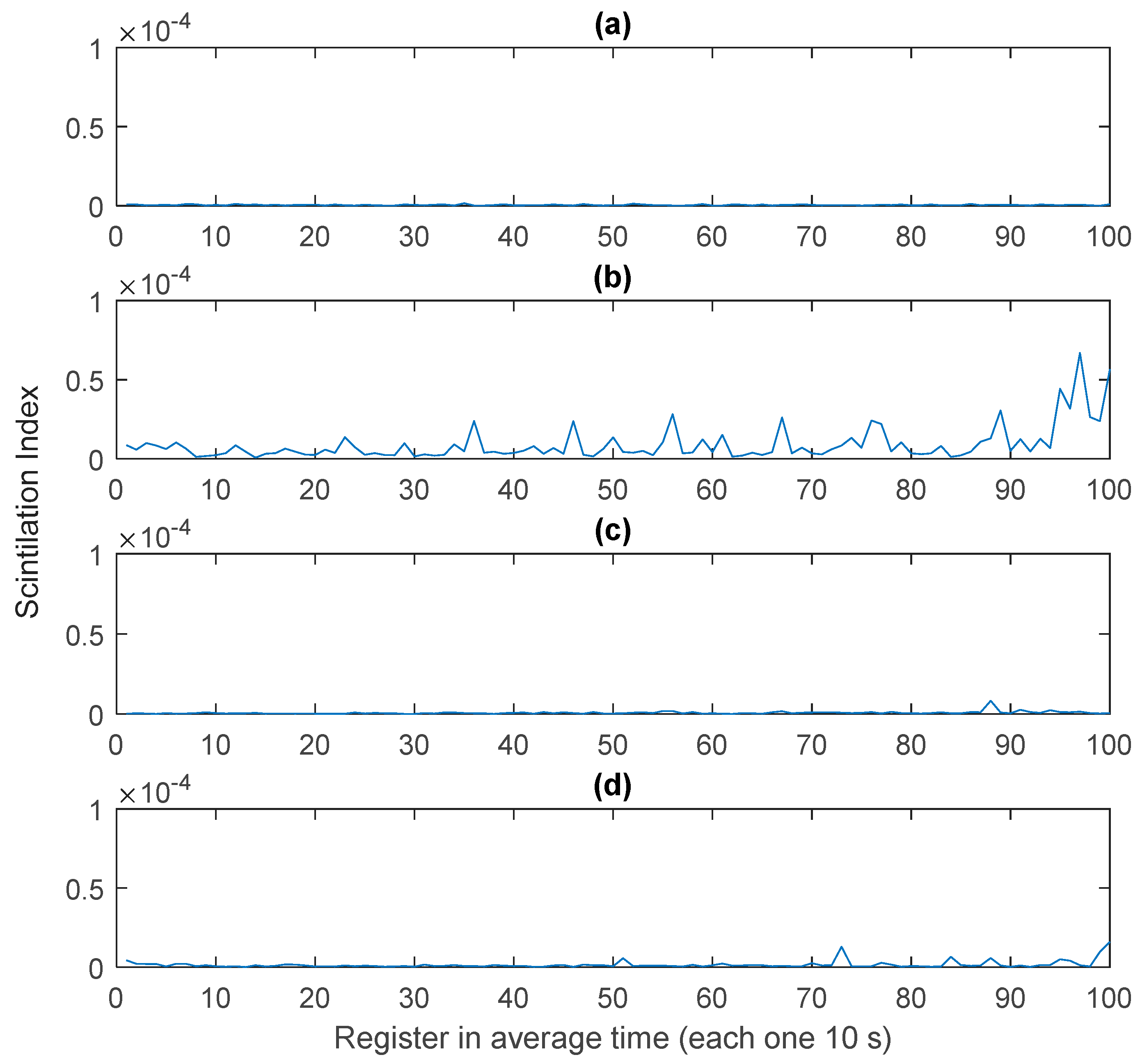
The fluctuation of the highest angle was found in Test #1, where the relative humidity was close to 100%. Even though the Pattern Test had shorter fluctuations than Test #1, we could not affirm, at this time, anything about a relationship between humidity and angle fluctuation. On the other hand, the scintillation index is computed from the acquired images using Equation (5), aside a constant factor calibrated from a power meter device. The outcomes are shown in Figure 14.

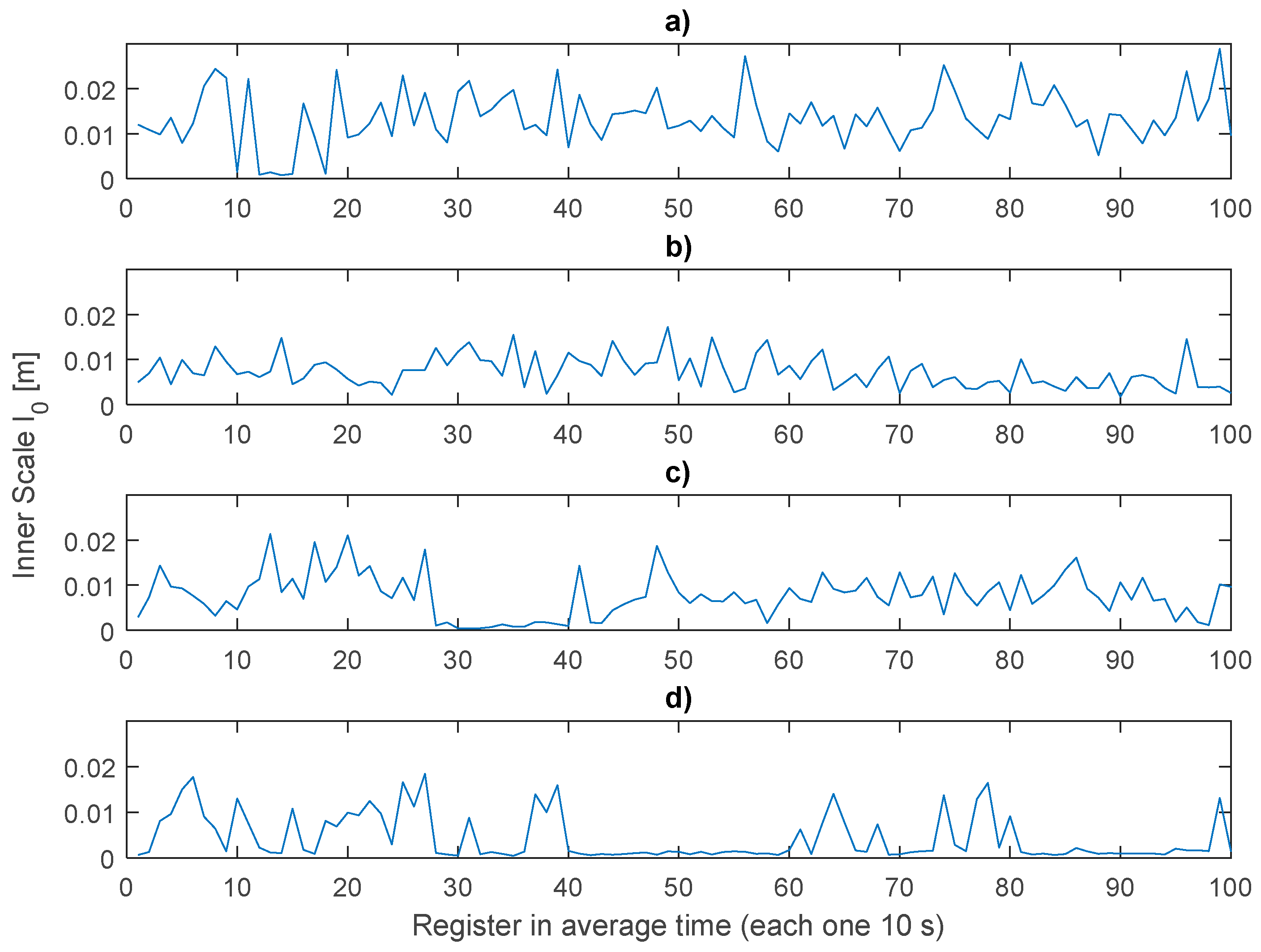
It can be observed on Figure 14 that the scintillation index was most stable in the Pattern Test; Test #1 had more variations, and both Test #2 and Test #3 had insignificant variation. Then, the inner scale $l_0$ is also computed from previous results and Equation (6), as shown in Figure 15.

Figure 15 shows Test #1 as the smallest inner scale which is an expected value because the inner scale must be small when turbulence is strong.

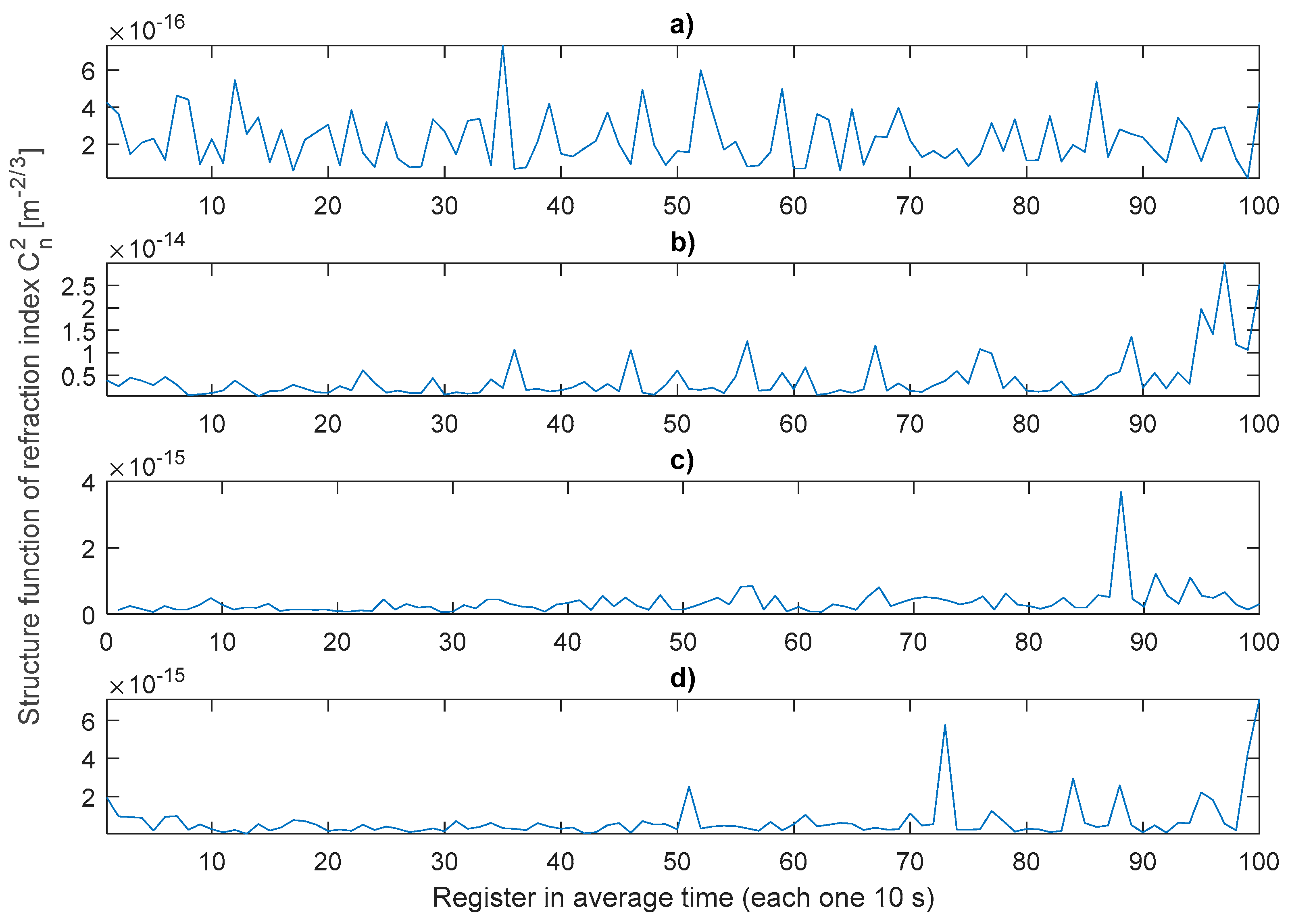
On the other hand, Table 4 shows final statistics for different turbulence parameters and Figure 16 the results of computing $C_n^2$, the refractive index structure constant.

In Figure 16, it was necessary to use a different scale in Test #1 to detail the values on the effect of turbulence in the other tests. In this case and using Equation (7), we could identify that the scale on Figure 16b is 10 times greater than its c and d.

Finally,

Table 5. Statistics of parameters to calculate $C_n^2$.

Test Name	${\mathit{C}}_{\mathit{n}}^2$ Average (${\mathit{m}}^{-2/3}$)	${\mathit{C}}_{\mathit{n}}^2$ Stand. Dev. (${\mathit{m}}^{-2/3}$)
Pattern	2.28 × 10−16	1.4 × 10−16
Test #1	4.05 × 10−15	4.91 × 10−15
Test #2	3.45 × 10−16	4.01 × 10−16
Test #3	6.95 × 10−16	1.01 × 10−15

shows the average and the standard deviation of the refractive index structure constant ($C_n^2$). Notice that Test #1 corresponds to a strong turbulence at a relative humidity of 99.13%.

4. Discussion

The techniques presented were implemented as a collaborative arrangement between electronic and optical devices. Temporal synchronization is important to ensure that each sample is taken under the frozen turbulence hypothesis. CMOS-1 and CMOS-2 were used to test the model and estimate centroids fluctuations as shown in Figure 7 and Figure 8. In addition, 2D histograms calculated to see temporal movements were a key to study the turbulence behavior.

Regarding previous results, devices were adapted to measure different turbulence parameters [7]. Besides, if only $C_n^2$ is observed, it is difficult—and perhaps impossible—to associate humidity changes to estimate the degree of turbulence. It means that the highest value of humidity corresponded to the moderate turbulence; on the other hand, in normal conditions observed at Pattern Test, the turbulence was weak, as well, while the other parameters were coherent with the relative humidity value.

5. Conclusions

This paper proposes a simple technique to change the relative humidity, isolated from the experimental setup, to measure its effects on an optical turbulence generator. This setup allows temporal fluctuations in the frontwave of the laser beam because of the controlled relative humidity inside the OTG. Fluctuations are computed from the centroids of images acquired at different horizontal distances from the laser output. In addition, the arrival angle and the intensity were computed from the experimental measurements. Other turbulence parameters had a behavior in accordance with the relative humidity changes (in line with the average values in Table 4). Further, the study used a laser beam propagated horizontally without a telescope, lens, or any other optic element, avoiding aberrations and high-cost devices. A scheme using an interferometer and a fringe pattern to compute the optical phase effect will be considered for future works.

References

- Kolmogorov, A.N. The local structure of turbulence in incompressible viscous fluid for very large Reynolds numbers. Proc. R. Soc. London. Ser. A Math. Phys. Sci. 1991, 434, 9–13. [Google Scholar] [CrossRef]
- Tatarski, V.I. Wave Propagation in a Turbulent Medium; Dover Publ.: Toronto, ON, Canada, 1961. [Google Scholar]
- Larry, L.C.; Philips, R.L. Laser Beam Propagation through Random Media; SPIE Optic.: Washington, DC, USA, 2005; Volume 2, ISBN 0819459488. [Google Scholar]
- Dashti, M.; Rasouli, S. Measurement and statistical analysis of the wavefront distortions induced by atmospheric turbulence using two-channel moire deflectometry. J. Opt. 2012, 14, 095704. [Google Scholar] [CrossRef]
- Rasouli, S.; Tavassoly, M.T. Application of moiré technique to the measurement of the atmospheric turbulence parameters related to the angle of arrival fluctuations. Opt. Lett. 2006, 31, 3276–3278. [Google Scholar] [CrossRef] [PubMed]
- Rasouli, S. Use of a moiré deflectometer on a telescope for atmospheric turbulence measurements. Opt. Lett. 2010, 35, 1470–1472. [Google Scholar] [CrossRef] [PubMed]
- Consortini, A.; Sun, Y.Y.; Innocenti, C.; Li, Z.P. Measuring inner scale of atmospheric turbulence by angle of arrival and scintillation. Opt. Commun. 2003, 216, 19–23. [Google Scholar] [CrossRef]
- Gustavo, F.; Garavaglia, M. Determinación de la Constantes de Estructura del Aire Turbulento Mediante Interferometría Young; Universidad Nacional de la Plata: Buenos Aires, Argentina, 2011. [Google Scholar]
- Jurado Navas, A.; Puerta Notario, A. Enlaces ópticos no Guiados con téCnicas de Diversidad en Canal AtmosféRico Afectado por Turbulencias; Universidad de Málaga: Malaga, Spain, 2010; Volume 43. [Google Scholar]
- Kwiecień, J. The effects of atmospheric turbulence on laser beam propagation in a closed space—An analytic and experimental approach. Opt. Commun. 2019, 433, 200–208. [Google Scholar] [CrossRef]
- Mckechnie, T.S. General Theory of Light Propagation and Imaging Through the Atmosphere; Rhodes, W.T., Ed.; Springer: Basel, Switzerland, 2016; ISBN 9783319182087. [Google Scholar]
- Herreño Vanegas, M.F.; Villamizar Conde, J. Estudio de los Efectos de la Humedad en la Caracterización de la Propagación de un haz láser a Través de la Turbulencia Atmosférica a Bajas Alturas en Trayectorias Horizontales; Universidad Industrial de Santander: Bucaramanga, Colombia, 2016; Volume 1. [Google Scholar]
- Hovis, J. What Causes Humidity? Available online: https://www.scientificamerican.com/article/what-causes-humidity/ (accessed on 13 December 2017).
- Tíjaro, O.; Galeano, Y.; Torres, Y. Method to measure effects of turbulence using CCD sensors and beam centroids. Laser Commun. Propag. through Atmos. Ocean. V 2016, 9979, 99790P. [Google Scholar] [CrossRef]
- Rhodes, W.T. Time-average Fourier telescopy: A scheme for high-resolution imaging through horizontal-path turbulence. Appl. Opt. 2012, 51, A11. [Google Scholar] [CrossRef] [PubMed]
- Meneses, J.; Gharbi, T.; Humbert, P. Phase-unwrapping algorithm for images with high noise content based on a local histogram. Appl. Opt. 2005, 44, 1207–1215. [Google Scholar] [CrossRef] [PubMed]
- Davis, J.I. Consideration of atmospheric turbulence in laser systems design. Appl. Opt. 1966, 5, 139–147. [Google Scholar] [CrossRef] [PubMed]
- Wilfert, O. Laser beam attenuation determined by the method of available optical power in turbulent atmosphere. J. Telecommun. Inf. Technol. 2009, 53–57. [Google Scholar]
- Spectra-Physics Model 107B/Model 127 (25 or 35 mW) Helium-Neon Lasers. 1996, pp. 1–4. Available online: http://www.asi-team.com/asi%20team/brookhaven/35mW-Laser.pdf (accessed on 1 September 2019).
- Optics, E. EO 1312C 1/1.8” CMOS Color USB Camera. 1992, 473. Available online: https://www.edmundoptics.com/p/eo-1312c-118-cmos-color-usb-camera/26850/ (accessed on 1 September 2019).
- Specialties, M. HTS2030SMD–Temperature and Relative Humidity Sensor. Available online: https://datasheet.octopart.com/HTS2030SMD-TE-Connectivity-datasheet-15992094.pdf (accessed on 1 September 2019).
- Arduino Platform. Available online: https://www.arduino.cc/ (accessed on 1 September 2019).
- Imaging Developem Systems, I. uEye ActiveX Control. Available online: https://en.ids-imaging.com/manuals-ueye-software.html (accessed on 3 September 2019).
- Holm, D.D. Taylor’s Hypothesis, Hamilton’s Principle, and the LANS-a Model for Computing Turbulence. Los Alamos Sci. 2005, 172–180. [Google Scholar]
- Labeyrie, A.; Lipson, S.G.; Nisenson, P. An Introduction to Optical Stellar Interferometry; Cambridge University Press: Cambridge, UK, 2006; ISBN 9780521828727. [Google Scholar]
Figure 1.
Signal processing scheme to register characteristics of beam centroid on an electronic embedded system. Source: Authors.
Figure 2.
Transversal shifts of laser propagation, the illustration shows two observers placed at and , at (solid line) and (dashed lines), respectively. We assumed a centered beam at time , and beam wander effects at time due to laser cavity (in polar coordinates). Source: Authors.
Figure 3.
Experimental setup. A#: Density neutral filter. BS#: Beam Splitter #. CMOS#: CMOS Camera to acquire beam at =1.18 [m], =1.45 [m] and =3.97 [m]. OTG: Optical Turbulence Generator. RHG: Relative Humidity Generator. Source: Authors.
Figure 4.
Scheme to compute the angle of centroids. Source: Authors.
Figure 5.
Designed board to add humidity signal to the microcontroller (ADC). Source: Authors.
Figure 6.
Signal processing scheme to register humidity fluctuations on an embedded system. Source: Authors.
Figure 7.
Temporal distribution, in cartesian coordinates, of centroid fluctuations to Pattern Test. Up: Measured at distance , Down: estimated at distance from distance and . (a) X-axis. (b) Y-axis. Source: Authors.
Figure 8.
2D histogram of temporal fluctuations in the Pattern Test (X and Y movements are in pixels). (a) Measured at distance . (b) Estimated at from distance and . Source: Authors.
Figure 9.
2D histogram of temporal fluctuations measured at : (a) Pattern Test. (b) Test #1. Source: Authors.
Figure 10.
2D histogram of temporal fluctuations measured at plane: (a) Pattern Test. (b) Test #2. Source: Authors.
Figure 11.
2D histogram of temporal fluctuations measured at plane: (a) Pattern Test. (b) Test #3. Source: Authors.
Figure 12.
Temporal distribution for the angle of the centroid for the Pattern Test, measured at the plane. Source: Authors.
Figure 13.
Fluctuations for the angle of centroid () according to Test: (a) Pattern. (b) Test #1. (c) Test #2. (d) Test #3. Source: Authors.
Figure 14.
Scintillation index () according to Test: (a) Pattern. (b) Test #1. (c) Test #2. (d) Test #3. Source: Authors.
Figure 15.
Inner Scale () according to Test: (a) Pattern. (b) Test #1. (c) Test #2. (d) Test #3. Source: Authors.
Figure 16.
Refraction index structure constant according to Test: (a) Pattern. (b) Test #1. (c) Test #2. (d) Test #3. Source: Authors.