Three-Dimensional Wind Measurements with the Fibered Airborne Coherent Doppler Wind Lidar LIVE

Abstract

A three-dimensional (3D) wind profiling Lidar, based on the latest high power 1.5 µm fiber laser development at Onera, has been successfully flown on-board a SAFIRE (Service des Avions Français Instrumentés pour la Recherche en Environnement) ATR42 aircraft. The Lidar called LIVE (LIdar VEnt) is designed to measure wind profiles from the aircraft down to ground level, with a horizontal resolution of 3 km, a vertical resolution of 100 m and a designed accuracy on each three wind vector components better than 0.5 m.s⁻¹. To achieve the required performance, LIVE Lidar emits 410 µJ laser pulses repeating at 14 KHz with a duration of 700 ns and uses a conical scanner of 30° total opening angle and a full scan time of 17 s.

1. Introduction

Since the late 1980s, several on-board coherent wind lidars have been developed, tested and exploited, based on various laser technologies, i.e., at 10.6 µm with a gas laser [1,2,3], and at 2 µm with a solid state laser [4,5,6]. Recent progress in fiber laser technology has enabled new lidar technology development [7,8,9,10]. More robust and compact fiber technology paves the way for the simple and standard use of coherent Doppler lidar from an airplane. The 1.5 µm lidar called LIVE (LIdar VEnt) has been developed at Onera in order to measure three-dimensional (3D) wind fields under an airplane. It was installed and tested on a SAFIRE (Service des Avions Français Instrumentés pour la Recherche en Environnement) ATR42 aircraft. LIVE wind lidar is based on a Leosphere lidar that has been extensively modified to meet the constraints of real-time wind measurement from an aircraft. In particular, it incorporates an innovative laser amplifier designed and developed by Onera which, thanks to its high peak power pulses, makes it possible to perform wind profiling from the aircraft altitude down to ground level.

2. Experiments

LIVE lidar has been designed for 3D wind profiling from an aircraft for meteorological applications. The wind measurement requirements are a horizontal resolution of 3 km, a vertical resolution of 100 m and an accuracy on each of the three wind vector components better than 0.5 m.s⁻¹.

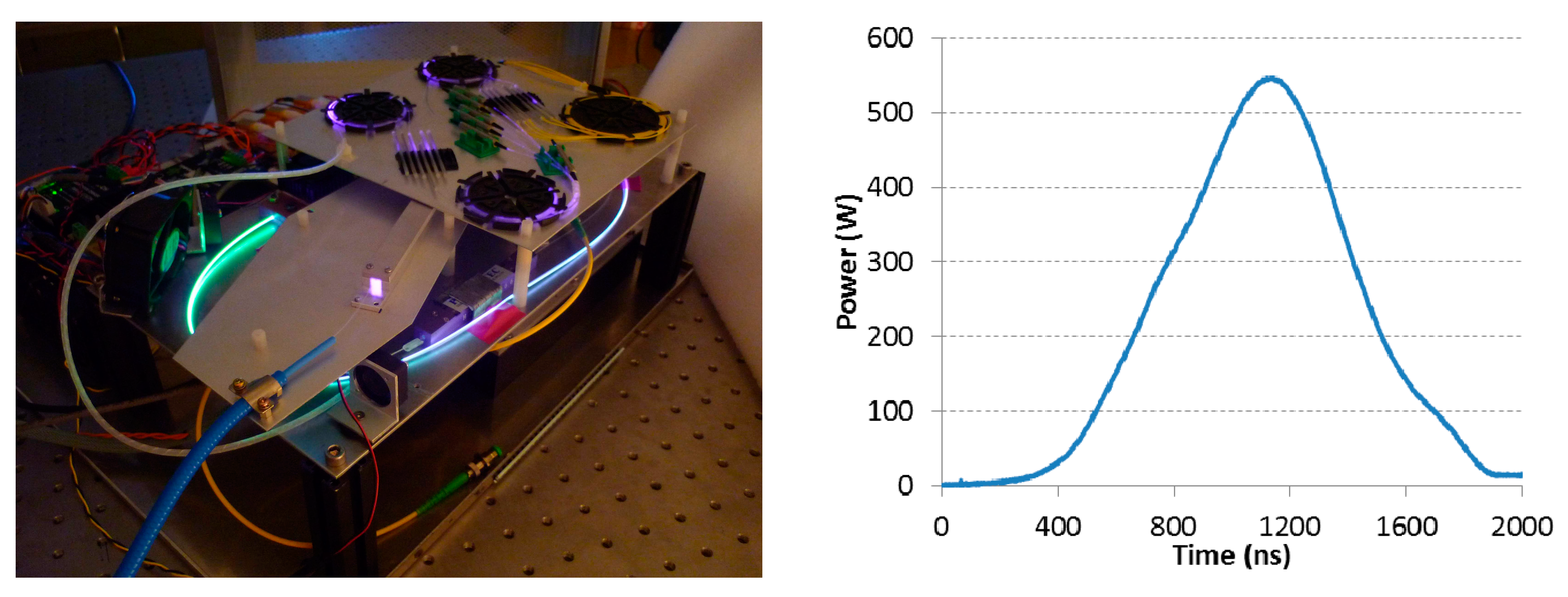
2.1. Fiber Laser Design

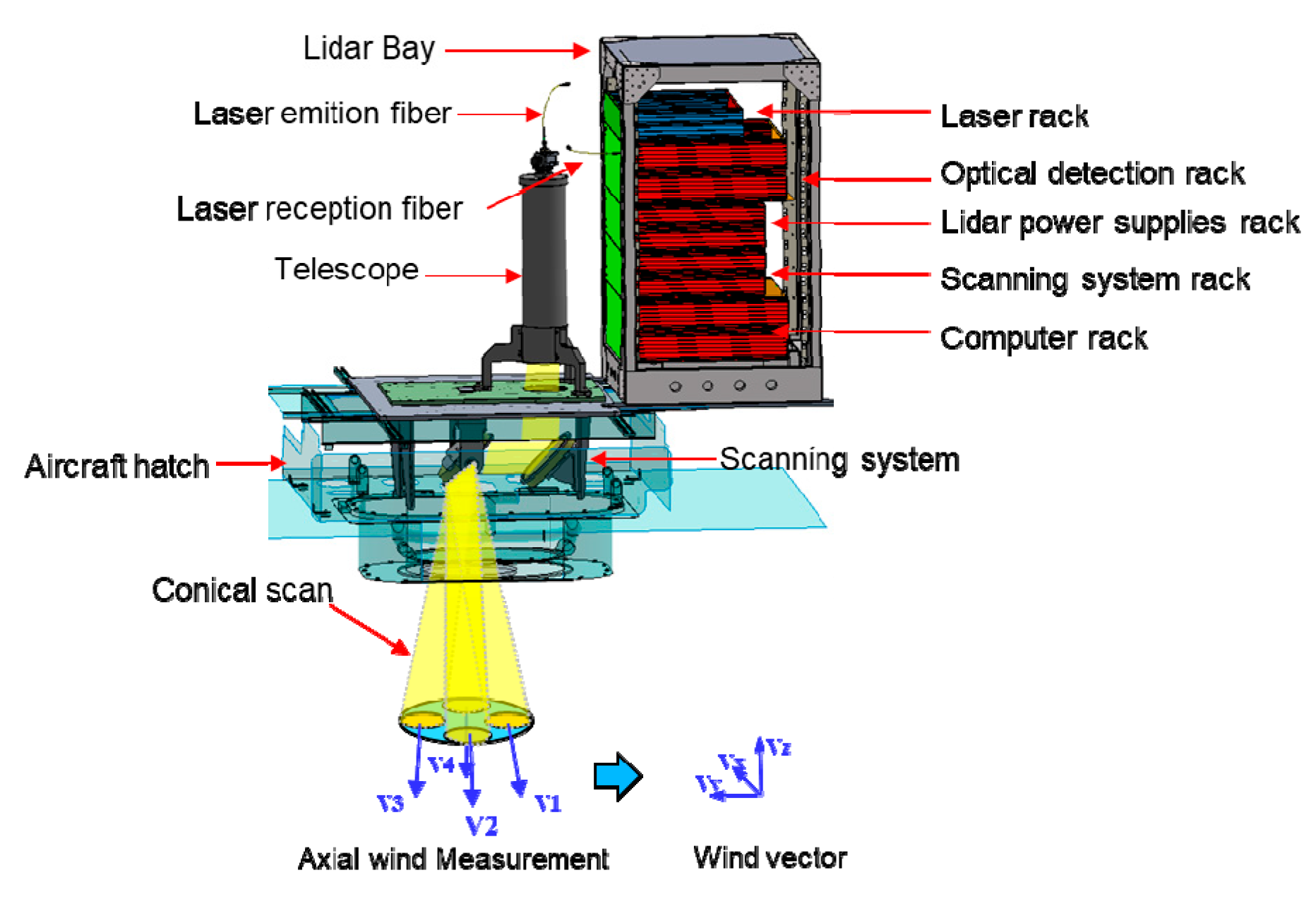
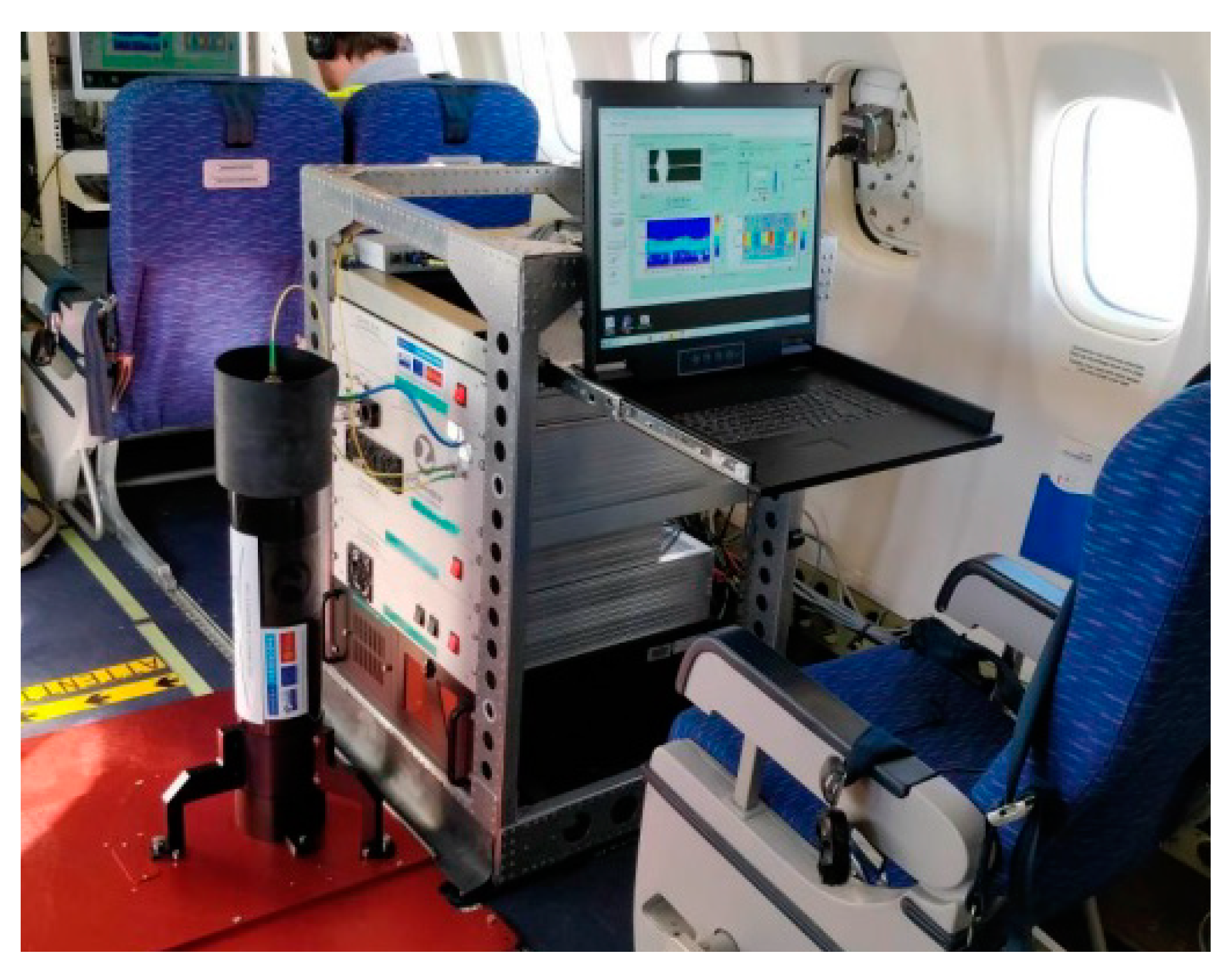
The laser source of the LIVE lidar is a pulsed 1.5 µm all-fiber laser based on master oscillator power amplifier architecture. To achieve the required accuracies for wind velocity measurement, the laser pulses should have an energy higher than 300 µJ and a duration of 700 ns. The coherent Doppler lidar application has additional requirements such as polarized laser emission, near-diffraction limited spatial beam quality and Fourier-limited spectral linewidth for coherent detection.

In fiber amplifiers, this last specification on linewidth limits the achievable laser energy, or more precisely, the achievable peak power. Indeed, to avoid nonlinear effects (particularly stimulated Brillouin scattering (SBS)), peak power must remain below the SBS threshold. Many methods have been experimented with to overcome this limitation, i.e., special fibers [11] or the use of a temperature or strain gradient along the amplifying fiber [12]. The simplest one from the lidar system point of view is the use of large mode area (LMA) fibers. In this case, the technical challenge is the fabrication of the amplifying fiber. The core diameter must be increased while reducing the numerical aperture to minimize the number of guided modes and maintain a quasi-single mode operation, since high beam quality is essential for lidar efficiency. In commercial pulsed power amplifiers at 1.5 µm, amplifying fibers are double-clad polarization maintaining Erbium–Ytterbium co-doped fibers. Two years ago, commercially available fibers of this type limited the peak power of a 700 ns pulse to 250–300 W when no SBS mitigation technic was implemented. A new glass matrix was proposed and after several tests, a new Erbium–Ytterbium co-doped fiber has been fabricated. This fiber enables us to reach a higher peak power, around 600 W, with all the necessary characteristics in terms of polarization maintenance, beam quality and amplification efficiency [13].

For the LIVE lidar, we developed the last power amplifier stage of the laser source with this new fiber and evaluated the laser performance. A picture of the laser is presented in Figure 1. The emission is linearly polarized, and we measured a polarization extinction ratio of 17 dB. An excellent beam quality is also observed with a measured beam quality factor M² = 1.1. Pulses were temporally shaped thanks to the acousto-optic modulator to compensate for distortions in the different amplification stages in order to obtain a duration of 715 ns and the pulse shape is presented in Figure 1. The pulse repetition frequency is 14 kHz and the pulse energy is limited by the SBS to 410 µJ. A double-pass architecture in the preamplifier enabled us to minimize ASE (Amplified Spontaneous Emission) generation and amplification in the power amplifier; a low level of ASE (<2%) is measured [14].

2.2. Lidar Design

LIVE Lidar has been designed to be compact, robust and suited to ATR42 aircraft integration. It was composed on an aircraft adapted bay that includes (see Figure 2):

• A rack for various Lidar power supplies.
• A control rack for the scanning system.
• A rack for the emission of the Lidar beam including the Onera laser source.
• A rack for the Lidar signal reception and its coherent detection.
• A rackable computer for real time processing.

The total power consumption is about 900 VA (Volt Ampere) and the weights of the scanning head and the lidar bay are 18 kg and 58 kg, respectively. The lidar bay is sufficiently compact to occupy a volume of 55 × 65 × 130 cm³.

The telescope is in a carbon tube positioned above the hatch of the aircraft on a metal interface plate that also supports the scanning system. Scanning for the analysis of the wind fields involves a system consisting of two mirrors to allow conical addressing. The beam emitted by the telescope is sent back to a fixed mirror and then to a mirror mounted on a gimbal-type scan turret as represented in Figure 2.

For a flight altitude of 5000 m, and an aircraft speed of 100 m.s⁻¹, the 3 km horizontal resolution is obtained with conical scanning with a total opening angle of 30° and one round in 17 s. After each lap, the lidar points in the nadir direction in 2 s in order to achieve good accuracy on vertical wind measurements.

The lidar is installed inside the SAFIRE ATR42 looking through a trapdoor in the floor of the plane in while aiming towards the nadir (Figure 3).

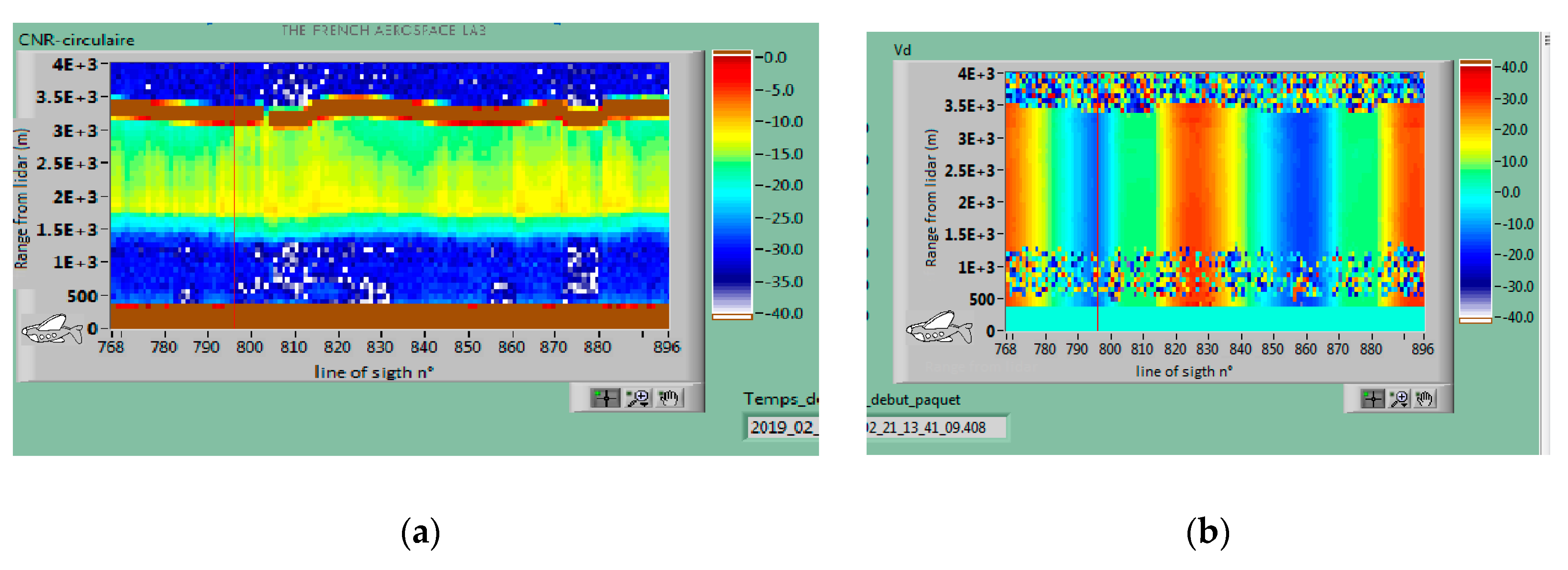
2.3. Lidar Signal Processing

Lidar raw data are first processed into spectrograms which show power spectral density as a function of lidar range on one axis and Doppler frequency on the other axis. Within a short time (0.3 s), called the line of sight time, the motion of the laser beam (6°) is considered small enough to be neglected. All computed spectrograms within this line of sight time are averaged in order to reduce noise. This task is made in real time using GPU (Graphics Processing Unit) computing. Such averaged spectrograms are computed for every line of sight of a full 360° scan. Thus, after a full scan, spectrogram data show power spectral density as a function of line of sight angle, lidar range and Doppler frequency.

From this stage, real time processing and post processing will differ. The aim of real time processing is to quickly deliver information about lidar measurement. The carrier to noise ratio (CNR) and radial wind speed are computed from spectrogram data at all lidar ranges and line of sight angles, using fast computing moments estimators along the Doppler frequency dimension. This CNR and radial wind speed data (functions of line of sight angle and lidar range) are displayed in real time by the lidar interface for monitoring purposes.

The aim of post processing is to offer the best performance. Since the aircraft will operate above the planetary boundary layer (PBL), the backscatter coefficient is expected to be a hundred times lower than usual at ground level. Therefore, the best low CNR estimators must be used for wind vector retrieval. According to [15], the usual algorithms such as velocity azimuth display (VAD) are limited at low CNRs; in essence, these algorithms use radial velocity data computed from the spectrogram in a way that is similar to real time processing. The limitation at low CNRs lies in the fact that each column of the spectrogram (along the Doppler frequency dimension) has been computed within a short time (of a line of sight). Thus, retrieving information at a column scale is not efficient in terms of low CNR performance. A more efficient algorithm would work with spectrogram data as a whole along the line of sight angle dimension.

According again to [15], two algorithms show excellent low CNR performance: the maximum of the function of the accumulated spectra (MFAS) and the wind vector maximum likelihood (WVML). For each lidar range, both algorithms compute the wind speed vector directly from spectrogram data along the Doppler frequency dimension and line of sight angle dimension. Both algorithms are complementary and are applied to our data during post processing.

The MFAS is, in essence, well suited for signal detection.

Figure 4 shows an example of low CNR spectrogram data obtained at high altitude (first range gate from the aircraft), which at first sight seems to contain only noise. The MFAS algorithm has detected the lidar signal, and its presence is highlighted by a trail of black dots. Lidar signal center frequency as a function of scan angle has a sinusoidal shape due to the projection of a constant wind vector on laser beam direction with conical motion. The phase of the sinusoidal shape is the direction of horizontal wind, its amplitude is proportional to the modulus of horizontal wind, and its offset from zero Doppler frequency is proportional to vertical wind. The MFAS algorithm makes rough assumptions about the value of horizontal wind (within the range of expected values). There is a sinusoidal shape for each assumption. As shown in Figure 5 on the left hand side, the MFAS algorithm shifts the spectrogram data of frequency in order to compensate for lidar signal center frequency dependence on scan angle. Then, the MFAS algorithm averages the compensated spectrogram data over all scan angle values, as shown in Figure 5 on the right hand side. If the assumption is roughly equal to the real value of horizontal wind, the accumulated spectra will exhibit a signal peak. The closer the assumption is from the real value, the stronger the signal peak, hence the name of the algorithm: maximum of the function of accumulated spectra. The remaining frequency offset from zero Doppler frequency leads to an estimate of vertical wind. Accumulated spectra also allow us to estimate the lidar CNR.

The accuracy of the MFAS algorithm is related to the number of assumptions being computed, i.e., the computing time allocated to the algorithm. It is wise to use a rough MFAS estimate in order to initiate a WVML algorithm dedicated to wind accuracy. The WVML algorithm is a more common algorithm which fits a wind parametric model over spectrogram data thanks to an optimization algorithm. We then proceeded with wind vector estimation for all lidar ranges.

At this stage, the wind has been estimated relative only to the aircraft. In order to obtain the wind relative to the ground, we must add aircraft speed relative to the ground (or cancel ground speed relative to the aircraft). The accuracy of aircraft attitude from FTI (Flight Test Instrumentation) and lidar orientation relative to the aircraft is not high enough to safely add aircraft speed. For an aircraft speed of 100 m.s⁻¹, an error of orientation of a single degree will lead to a residual aircraft speed of 1.75 m.s⁻¹ on axes perpendicular to aircraft motion. The desired wind speed accuracy is 0.5 m.s⁻¹, and this goal requires a precise ground speed relative to the aircraft cancelling procedure. We have chosen to work with ground speed measured from the lidar ground level return. Since both measurements are done within the same frame of reference, there is no lidar orientation issue. As the signal level from the ground return is stronger than the signal level from the atmospheric return, we use a more common VAD algorithm to retrieve ground speed relative to the aircraft.

3. Results

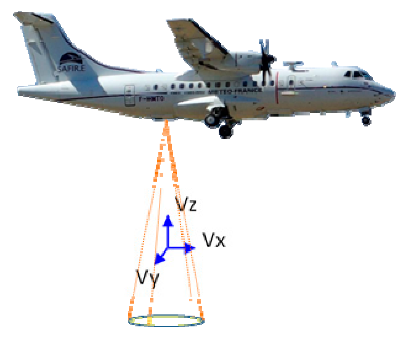
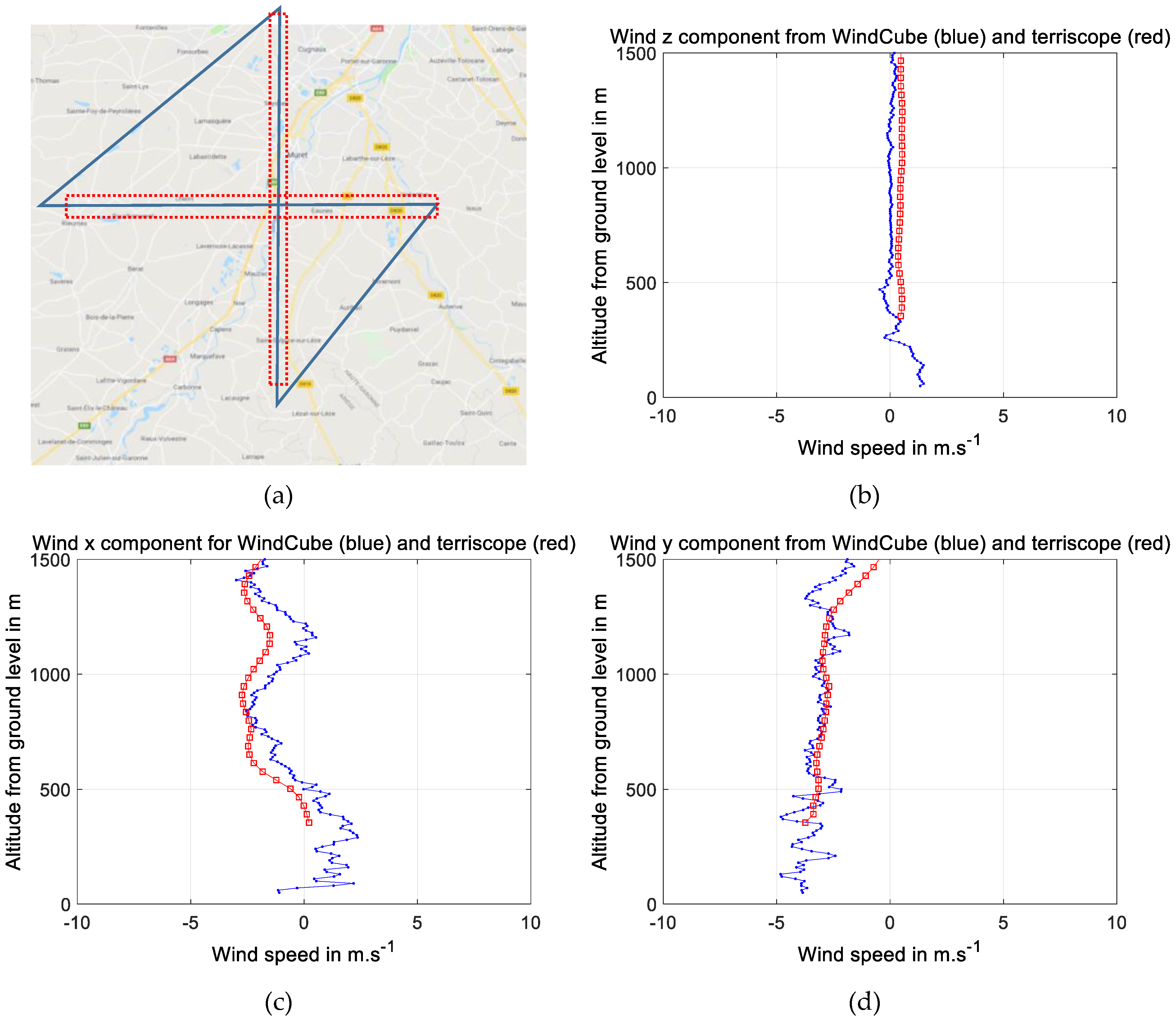
3.1. Flight Test Campaign

Objectives of the test campaign were to evaluate LIVE lidar behavior in an aeronautical environment, to validate its performance (range and velocity measurements), and to validate LIVE 3D wind field measurements by comparisons with wind measurements from other ground based wind profilers, such as ultra high frequency (UHF) radar and ground based lidar.

Acquisitions of LIVE lidar took place on 20, 21 February 2019, during two flights over two geographical areas of interest: a mountainous area around the city of Lannemezan and a plain area around the city of Fauga. Near Lannemezan, the Atmospheric Research Center (CRA) had two radar wind profilers operating, an UHF and a very high frequency (VHF) radar. Their data will enable Lidar measurements to be validated at high altitudes. Near Fauga, Onera has a center where a WindCube 100S (commercial Lidar from Leosphere) was operated to compare ground based lidar with airborne lidar measurements in the boundary layer. Flight altitudes of 3 km, 5 km and 7 km were used during these flight tests. Figure 6 shows LIVE lidar installed inside the ATR42 of SAFIRE, with a red aluminum plate covering the hole in the aircraft floor over the rear bottom porthole. Under this plate is the gimbal deflection turret, and over it is the lidar telescope. All optical electronic components are inside the grey racks of the bay, with the black computer on the bottom and its display deployed for operator use on top.

As explained in the lidar signal processing chapter, displays for a short time (0.3 s) averaging of CNR and velocity along the line of sight are processed in real time thanks to GPU computing (Figure 7). The CNR is a useful coherent lidar signal quality criterion [16]. In the usual case of detection noise being limited by shot noise, the accuracy of the measured wind speed is theoretically proportional to:

$${\sigma }_v=\frac{1}{f\left(CNR\right)\sqrt{N}},$$

(1)

where N is the number of averaged pulses and f is an increasing function depending on lidar configuration.

Figure 7 shows an example of the on-board real time display. Figure 7a shows the real time display of CNR: the horizontal axis is the line of sight number (the real time display shows two complete conical scanning patterns) and the vertical axis is the range from the lidar. The CNR display first exhibits a blind zone due to the reflection of the laser pulse on the optics, followed by a low CNR area (in blue) due to low aerosol density at high altitudes. Then, the laser pulse reaches the top of the boundary layer at 1.5 km from the lidar, and a high level of lidar signal is obtained to the ground, where a strong reflection occurs at 3.3 km from the lidar. The distance from which ground reflection is obtained varies because of landforms. Figure 7b shows the real time display of wind velocity versus line of sight number. The velocity display shows a rainbow pattern mainly due to aircraft speed projection on the conical scan of the line of sight. At 700 m to 1200 m from the lidar, the real time velocity display contains many outliers due to low CNR in this range.

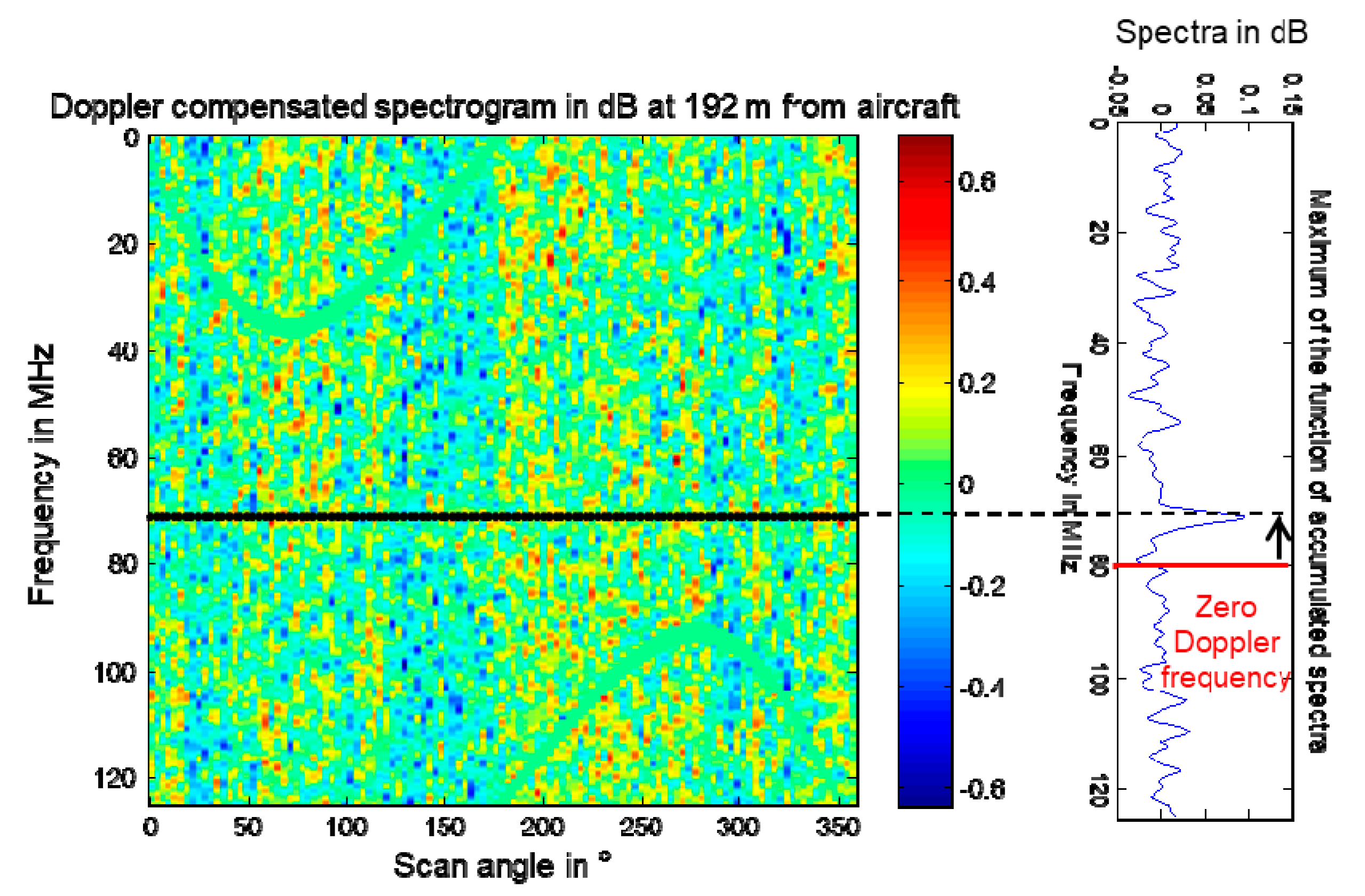
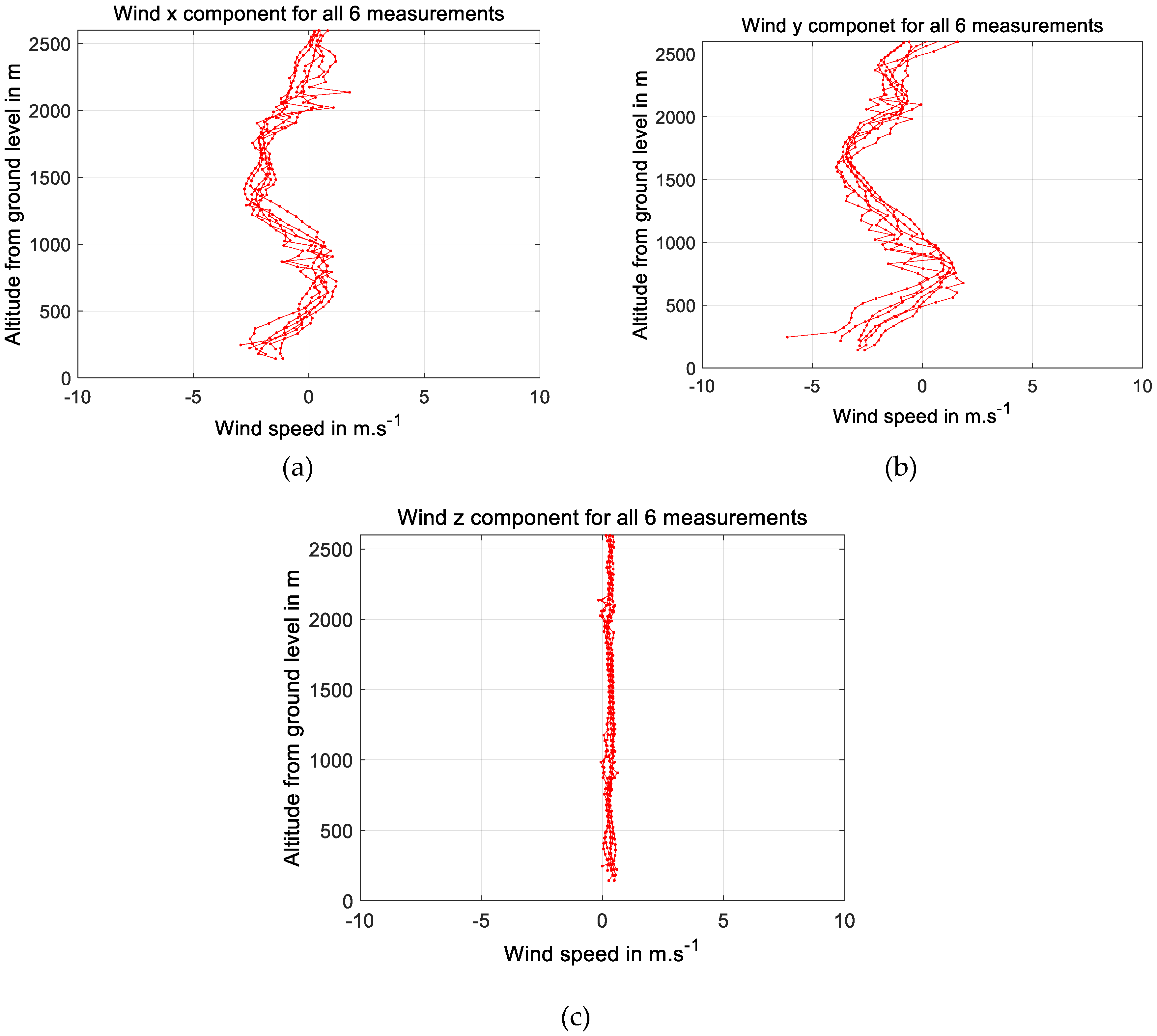
3.2. Flight Test Results

Raw data from the flight tests were stored for post processing. As explained in the lidar signal processing chapter, MFAS and WVML algorithms [15] are used for wind vector retrieval. These wind speed vectors, relative to the aircraft frame of reference, are then transposed to the earth frame of reference using FTI data (aircraft altitude, location and attitude). Since wind speed measured by lidar is the wind speed relative to the aircraft, we also add aircraft speed relative to the ground in order to calculate wind speed relative to ground.

Figure 8a shows the flight path (blue line) followed by the aircraft above the Onera ground based WindCube lidar near the city of Fauga. On 20 February 2019, the aircraft was flying over the ground based lidar at three different altitudes (FL100, FL160 and FL220), with two different headings for each altitude (red dashed boxes). Unfortunately, we got poor signal return from the WindCube on this day. The next day (21 February 2019), the aircraft only flew at FL100 and we were able to receive a signal from the WindCube up to the top of the planetary boundary layer. Figure 8b–d shows the comparison between LIVE (red squared line) and WindCube (blue dotted line) wind measurements for all three components in the earth frame of reference. The agreement between the two lidars is good, considering that the 2 km footprint of LIVE is larger than the one of WindCube. The accuracy of the WindCube as given by its manufacturer is 0.2 m.s⁻¹ in radial wind speed in the range of 100 m to 2 km.

In the lidar signal processing chapter, we have also mentioned an orientation issue between LIVE lidar and FTI when we add the aircraft speed relative to ground to the wind speed relative to aircraft. As a workaround, we have chosen to measure aircraft speed relative to ground also from LIVE lidar. In order to evaluate the quality of the workaround, we have compiled all six LIVE measurements of February the 20th of 2019 into Figure 9, from ground level up to FL100. Results are consistent despite a delay of almost a quarter of an hour between each measurement, and different aircraft orientations (heading, angle of attack varying with altitude).

4. Conclusions

An airborne 3D wind profiling lidar based on the latest 1.5 µm fiber laser development at Onera has been designed to be operated on-board an ATR42 aircraft from SAFIRE. The lidar includes a conical scanner aiming at the nadir. The horizontal resolution is 3 km for a flight altitude of 5000 m, the vertical resolution is 100 m and the designed accuracy on each three wind vector components is better than 0.5 m.s⁻¹. The CNR and line of sight velocity are displayed on-board in real time, and 3D wind vector retrieval is obtained from data post processing using the best low CNR algorithms.

A flight test campaign was successfully performed during February 2019. Airborne wind measurements are in good agreement with measurements from a WindCube lidar operated at Onera center in Fauga. Measurements from different headings and angles of attack are also consistent, showing that all procedures to transpose wind measurements relative to the aircraft into wind measurements relative to the ground are successful thanks to the use of aircraft speed extracted from on-board lidar measurements. Lidar measurement comparison with radar wind profile measurements from CRA are currently in progress.

This airborne wind fibered lidar is now available for meteorological and atmosphere dynamics scientific studies.

References

1. Bilbro, J.; Fichtl, G.; Fitzjarrald, D.; Krause, M.; Lee, R. Airborne Doppler lidar wind field measurements. Bull. Am. Meteorol. Soc. 1984, 65, 348–359. [Google Scholar] [CrossRef]
2. Targ, R.; Kavaya, M.J.; Huffaker, R.M.; Bowles, R.L. Coherent lidar airborne windshear sensor: Performance evaluation. Appl. Opt. 1992, 30, 2013–2026. [Google Scholar] [CrossRef] [PubMed]
3. Reitebuch, O.; Werner, C.; Leike, I.; Delville, P.; Flamant, P.H.; Cress, A.; Engelbart, D. Experimental Validation of Wind Profiling Performed by the Airborne 10-μm Heterodyne Doppler Lidar WIND. J. Atmos. Ocean. Technol. 2001, 18, 1331–1344. [Google Scholar] [CrossRef]
4. Targ, R.; Hawley, J.G.; Steakley, B.C.; Ames, L.L. Airborne lidar wind detection at 2 µm. Proc. SPIE 1995, 2464, 109–115. [Google Scholar]
5. Targ, R.; Steakley, B.C.; Hawley, J.G.; Ames, L.L.; Forney, P.; Swanson, D.; Stone, R.; Otto, R.G.; Zarifis, V.; Brockman, P.; et al. Coherent lidar airborne wind sensor II: Flight-test results at 2 and 10 μm. Appl. Opt. 1996, 35, 7117–7127. [Google Scholar] [CrossRef] [PubMed]
6. Weissmann, M.; Busen, R.; Dörnbrack, A.; Rahm, S.; Reitebuch, O. Targeted observations with an airborne wind lidar. J. Atmos. Ocean. Technol. 2005, 22, 1706–1719. [Google Scholar] [CrossRef]
7. Dolfi-Bouteyre, A.; Augere, B.; Besson, C.; Canat, G.; Fleury, D.; Gaudo, T.; Goular, D.; Lombard, L.; Planchat, C.; Valla, M.; et al. 1.5 μm all fiber pulsed lidar for wake vortex monitoring. In Proceedings of the 2008 Conference on Lasers and Electro-Optics and 2008 Conference on Quantum Electronics and Laser Science, San Jose, CA, USA, 4–9 May 2008. [Google Scholar]
8. Kameyama, S.; Ando, T.; Asaka, K.; Hirano, Y.; Wadaka, S. Compact all-fiber pulsed coherent Doppler lidar system for wind sensing. Appl. Opt. 2007, 46, 1953–1962. [Google Scholar] [CrossRef] [PubMed]
9. Liu, J.; Zhu, X.; Diao, W.; Zhang, X.; Liu, Y.; Bi, D.; Chen, W. All-Fiber Airborne Coherent Doppler Lidar to Measure Wind Profiles. EPJ Web Conf. 2016, 119, 10002. [Google Scholar] [CrossRef] [Green Version]
10. Dolfi-Bouteyre, A.; Canat, G.; Lombard, L.; Valla, M.; Durécu, A.; Besson, C. Long-range wind monitoring in real time with optimized coherent lidar. Opt. Eng. 2016, 56, 031217. [Google Scholar] [CrossRef]
11. Canat, G.; Jetschke, S.; Lombard, L.; Unger, S.; Bourdon, P.; Kirchhof, J.; Dolfi, A.; Jolivet, V.; Vasseur, O. Multifilament-core fibers for high energy pulse amplification at 1.5 µm with excellent beam quality. Opt. Lett. 2008, 33, 2071–2073. [Google Scholar] [CrossRef] [PubMed]
12. Zhang, X.; Diao, W.; Liu, Y.; Liu, J.; Hou, X.; Chen, W. Single-frequency polarized eye-safe all-fiber laser with peak power over kilowatt. Appl. Phys. B 2014, 115, 123–127. [Google Scholar] [CrossRef]
13. Durécu, A.; Bourdon, P.; Gustave, F.; Jacqmin, H.; le Gouët, J.; Lombard, L. High Peak Power Single-Frequency Amplifier Based on a Er-Yb Doped Polarization Maintaining LMA Fiber. Opt. Soc. Am. 2018, 120. [Google Scholar] [CrossRef]
14. Durécu, A.; Pureur, V.; Cariou, J.; le Gouët, J.; Lombard, L.; Bourdon, P. High Peak Power Single-Frequency ASE-reduced PM LMA fiber amplifier. In Proceedings of the European Conference on Lasers and Electro-Optics 2017, Munich, Germany, 25–29 June 2017. [Google Scholar]
15. Smalikho, I. Techniques of wind vector estimation from data measured with a scanning coherent Doppler lidar. J. Atmos. Ocean. Technol. 2003, 20, 276–291. [Google Scholar] [CrossRef]
16. Lombard, L.; Valla, M.; Planchat, C.; Goular, D.; Augère, B.; Bourdon, P.; Canat, G. Eyesafe coherent detection wind lidar based on a beam-combined pulsed laser source. Opt. Lett. 2015, 40, 1030–1033. [Google Scholar] [CrossRef] [PubMed]
Figure 1. Left: picture of the power amplifier. Right: temporal shape of laser pulse.
Atmosphere 10 00549 g001
Figure 2. Diagram of the LIVE lidar installation inside the airplane. V1, V2 … represent radial wind speed measured by lidar, and Vx, Vy and Vz are the components of the retrieved wind vector.
Atmosphere 10 00549 g002
Figure 3. ATR42 aircraft, with trapdoor localization and lidar scanning representation.
Atmosphere 10 00549 g003
Figure 4. Spectrogram data at a low carrier to noise ratio (CNR), and presence of the lidar signal (black dotted trail) in accordance with the maximum of the function of the accumulated spectra (MFAS) algorithm estimation.
Atmosphere 10 00549 g004
Figure 5. Doppler compensated spectrogram and presence of lidar signal (black dotted trail) in accordance with MFAS estimation (left). Function of accumulated spectra (right).
Atmosphere 10 00549 g005
Figure 6. Picture of LIVE lidar installed inside the ATR42.
Atmosphere 10 00549 g006
Figure 7. (a) Line of sight CNR real time display. (b) Line of sight velocity real time display for the conical scan. Range zero is the aircraft altitude while range 3500 m is the ground echo.
Atmosphere 10 00549 g007
Figure 8. (a) Aircraft trajectories during measurements (north–south and west–east) over Fauga. (bd) respectively z (zenith), x (north) and y (west) components of wind measured by airborne lidar LIVE (red squares) and WindCube lidar (blue dots).
Atmosphere 10 00549 g008
Figure 9. (ac) respectively x (north), y (west) and z (zenith) components of wind measured by airborne lidar LIVE at three different altitudes and each altitude at two different headings.
Atmosphere 10 00549 g009