Abstract
The objective of this paper is to use remote sensing to measure on-road emissions and to examine the impact and usefulness of additional measurement devices at three sites. Supplementing remote sensing device (RSD) equipment with additional equipment increased the capture rate by almost 10%. Post-processing of raw data is essential to obtain useful and accurate information. A method is presented to identify vehicles with excessive emission levels (high emitters). First, an anomaly detection method is applied, followed by identification of cold start operating conditions using infrared vehicle profiles. Using this method, 0.6% of the vehicles in the full (enhanced) RSD data were identified as high emitters, of which 35% are likely in cold start mode where emissions typically stabilize to low hot running emission levels within a few minutes. Analysis of NOx RSD data confirms that poor real-world NOx performance of Euro 4/5 light-duty diesel vehicles observed around the world is also evident in Australian measurements. This research suggests that the continued dieselisation in Australia, in particular under the current Euro 5 emission standards and the more stringent NO2 air quality criteria expected in 2020 and 2025, could potentially result in local air quality issues near busy roads.
Keywords:
remote sensing; on-road; emissions; motor vehicle; road traffic; cold start; high emitter; NOx; NO2 1. Introduction
Motor vehicles are a major source of air pollution and greenhouse gas (GHG) emissions in urban areas around the world. The close proximity of motor vehicles to the general population makes this a particularly relevant source from an exposure and health perspective [1].
A comprehensive measurement of vehicle emissions in urban networks is cost-prohibitive due to the large number of vehicles that operate on roads with different emission profiles, large spatial and temporal variability in vehicle activity, and a range of real-world factors that influence emission levels [2]. Several methods are used to measure vehicle emissions, such as on-board emission measurements (PEMS), remote sensing, near-road air quality measurements, and tunnel studies. However, all methods have their own strengths and weaknesses, and the weaknesses in particular must be clearly understood and explicitly considered in any subsequent use of the emissions data, e.g., model development and validation [3].
Following on from earlier remote sensing work [4,5], the objective of this paper is to use remote sensing to measure on-road emissions and to examine the impact and usefulness of additional measurement devices. This study took a step further than ‘conventional’ remote sensing programs, with the specific aim to examine data accuracy, enhance data capture rates, and potentially address specific issues (bias) that relate to the use of remote sensing. The particular focus of this paper is on improving remote sensing device (RSD) capture rate, high emitter detection, (on-road) cold start detection, and trends in measured NO vehicle emissions.
2. Methods
2.1. Site Selection
An on-road measurement campaign was conducted at three locations in Brisbane, Australia. The sites were selected to represent different types of adjoining land use and therefore distinct situations regarding fleet mix and driving behavior. The sites were a freeway on-ramp (FWY) (Macgregor 4–5 September 2018), a heavily trafficked urban road (URB) (Taringa 6–7 September 2018), and a commercial road in an industrial area (COM) (Eagle Farm 20 February 2019). Figure 1 shows the test sites.
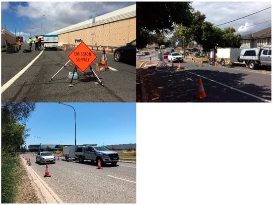
Figure 1.
On-road emission test sites in Brisbane, Australia, from left to right and down: freeway on-ramp (FWY) (4–5 September 2018), a heavily trafficked urban road (URB) (6–7 September 2018), and a commercial road in an industrial area (COM) (20 February 2019).
2.2. On-Road Instruments and Procedures
Different types of instrumentation were used to measure emissions, local air quality, and traffic activity and performance. Table 1 presents an overview of equipment used for each site. All sites were instrumented with a remote sensing device (RSD), a dedicated second license plate camera and a thermal imaging camera. On two sites, loop detectors and a network of Bluetooth MAC address units were also installed. On one site, two integrated air quality monitoring stations and speciated VOC sampling equipment were also used. In addition, two test vehicles were tested on a dynamometer and then driven multiple times past the RSD at one site.

Table 1.
Overview of equipment used at each measurement site.
An Accuscan RSD4600 was used to measure vehicle emission concentrations of CO, NO, HC, ‘UV smoke’, and CO2, and includes a Source Detector Module (SDM), a speed-acceleration bar, and a video camera to capture an image of the vehicle’s license plate number (LPN) [6]. The remote sensing system uses the principle that the majority of gases will absorb light at particular wavelengths. It measures on-road emissions by absorbance of ultraviolet (UV) and infrared (IR) light across an open (optical) path using wave-length specific detectors for different air pollutants. The RSD consists of an IR component for detecting CO, CO2, and HC, together with an UV spectrometer for measuring NO.
A specialized license plate number camera (Reconyx MS7 Microfire, Holmen, Wisconsin, USA) was installed about 15 m upstream from the RSD to provide complete information of the on-road traffic composition. In addition, a thermal imaging camera (Noptic Thermal Camera, Strategic Innovations, STH1000, Strategic Innovations, Melbourne, Australia) was used at the RSD site to record, visualize, and analyze the thermal profiles of individual vehicles.
Three sets of automatic pneumatic loop detectors were installed at two sites for a period of two weeks to collect traffic count data and speed and acceleration data for individual vehicles (refer to Section 3.3). Rubber tubes are placed across traffic lanes and when a pair of wheels hits the tube, air pressure in the compressed tube activates a recording device that notes the time of the event. Based on the pattern of these times, the device will match each compression event to a particular vehicle according to a vehicle classification scheme. Two tubes attached to the same counter can be placed a set distance apart in order to determine speed by measuring the interval between the time an axle hits the first tube and the time it hits the second tube. The loop pairs (i.e., two closely spaced loops) had a separation distance of 1 m. The distance between the loop pairs was 15 m and 20 m for the URB and FWY sites, respectively. The middle loop set was located as close to the RSD acceleration/speed bar as possible (about 2 m upstream). Data loggers were set to an atomic clock.
Bluetooth MAC address units were installed in the road network around the measurement sites, with the aim of tracking individual vehicle movements in time and space before the RSD measurement took place.
Two integrated air quality monitoring stations (AQM65) were installed at one site (URB), 7 m upstream of the RSD SDM and on both sides of the road (1 m from road markings and on the kerb) to monitor on-road minute-by-minute ambient concentrations. Local meteorology (wind speed/direction, temperature, humidity, etc.) was measured using a Vaisala WXT520. Summa canisters were also installed on site to provide VOC speciation of on-road emissions. The air quality results are discussed in a separate paper.
A portable transient vehicle dynamometer (Mustang Model MD1000, Twinsburg, Ohio, USA) was used to measure instantaneous emissions of two test vehicles (MY 2016 Euro 4 diesel 4WD Ford Ranger and a MY 2017 diesel Euro 5 4WD Ford Ranger). The same test vehicles were also driven multiple times past the RSD. A special driving cycle was developed specifically for this study. The dynamometer emission testing results are discussed in a separate paper.
3. Results and Discussion
The collective set of measurements provides a rich and unique database that can be analyzed in various ways. This paper presents the results of selected and specific analyses. The reader is referred to the following papers: (1) detecting cold start vehicles using thermal imaging and Bluetooth units [7] and (2) on-road air quality and remote sensing [8].
3.1. The Remote Sensing Database
Vehicle emission RSD measurement requires valid concentration and valid speed-acceleration readings, as well as a clear image of the license plate. The latter is required to retrieve essential information regarding vehicle class (e.g., vehicle type, fuel type, weight) and vehicle technology (year of manufacture, Euro standard). Other information such as vehicle make/model and residential address can also be useful, allowing for specific data analysis.
A total of 13,011 vehicles were measured by the RSD at the three sites, with 8813 valid emission and speed/acceleration measurements (68%) and 8194 valid samples with recorded license plate numbers (63%). Cross-referencing LPNs with the Queensland vehicle registration database resulted in 7889 vehicles with a valid LPN, i.e., a 61% overall capture rate in the RSD data, defined as a proportion of the total number of RSD samples. As a large portion (~40%) of the RSD measurements could not be used, reduction of data loss using additional equipment was examined.
3.2. Reduced Data Loss Using a Second Camera
The RSD measurements include a subset of valid concentration and speed-acceleration readings, but invalid RSD vehicle images. RSD images can be illegible (e.g., dirty LPN) or out of view. In fact, 619 RSD measurements (5%) had valid emissions and speed/acceleration readings but the LPN could not be retrieved from the RSD image.
The second LPN (Reconyx) camera is located further away from the road. It provides good picture quality and has a wider view. Hence, it is able to capture vehicles that are out of view for the RSD camera or suffer from poor picture quality.
Images taken with the specialized license plate camera were used to both verify and supplement the RSD database. Vehicle images collected by both the RSD and LPN camera were put through an automated LPN recognition process. The Open Automatic License Plate Recognition ALPR [9] open source software library was used to automate the identification of vehicle number plates from a total of 65,046 images (RSD 13,009 and LPN Camera 52,037 images) within a Microsoft Windows operating environment. The Open ALPR API was chosen for its advanced configuration options and availability in many popular software languages. Adobe Photoshop was used to pre-process images in order to convert images to grayscale and increase the levels of contrast and brightness to improve readability by Open ALPR. Python was used to automate the collection of the output from Open ALPR, extract image file metadata, and summarize results into CSV format. The process was completed with a manual check where missing LPNs were determined by visual inspection of the images.
The dedicated LPN camera provided LPN information for an additional 541 vehicles, leading to reduced data loss and an increase in overall RSD capture rate from 8194 vehicles (63%) to 8735 vehicles (67%). Only 78 vehicles remained with valid emissions and speed/acceleration readings, but without LPN information. It is noted that the second camera may also reduce potential bias in the RSD database, as vehicles missed by the RSD could be dominated by older dirtier and/or smoky vehicles.
3.3. Reduced Data Loss Using Vehicle Loop Detectors
Automatic loop detectors provide vehicle count and vehicle speed data. Acceleration can be computed for individual vehicles using the recorded (change in) speed values across the three loop detector sets. Raw loop speed and count data were post-processed to link the loop and RSD databases. R code was written to time-align and combine the relevant data (time stamp, speed, vehicle class, and wheel-base) from three individual loop sets at each site and subsequently determine speed and acceleration values for individual vehicles. The code specifically deals with data gaps that occur randomly in the loop detector data using a set of predefined rules. The rules are: (a) vehicle time stamps must be sequential in time when a vehicle moves from loop set 1 to 3, (b) time differences must be within a pre-determined vehicle speed-dependent tolerance, and (c) the measured wheel base must be within 4% of the mean value for each individual vehicle.
For the Urban and Freeway on-ramp sites the RSD collected 810 valid concentration measurements with invalid (or missing) speed and acceleration readings, representing a significant loss of data (7%). The loop detectors provided data for an additional 611 vehicles of which 584 had valid LPNs. Hence, RSD capture rate for the two sites increased significantly. In principle, loop detector data can be used to provide valid speed and acceleration data for these missed vehicles.
3.4. Expanded Remote Sensing Database
Before expansion, the RSD database with 13,011 records contained 7889 vehicles with valid measurement data. This corresponds to a 61% capture rate, which is defined as a proportion of the total number of RSD samples. The second LPN camera increased the capture rate to 65% and the loop detector speed/acceleration data increased this further to 69%. As a consequence, valid RSD emissions data were collected for a total of 8991 vehicles. This is a good overall result since capture rates for RSD studies are typically about 30–70% (NIWA, 2015).
3.5. Vehicle Counts Using Multiple Instruments
RSD does not capture all vehicles passing the RSD, i.e., a variable proportion of the on-road fleet is missed. The extent depends on traffic conditions (fleet mix, level of congestion, etc.) and weather conditions (rain, overcast/sunny, time of day, etc.). This means that the actual capture rate in terms of the on-road fleet is lower than the capture rate that is commonly defined as the proportion of all recorded RSD measurements.
To examine the significance of this issue, RSD ‘vehicle counts’ were cross-checked and compared with two independent measurement devices, i.e., loop detector count data and Reconyx ‘vehicle counts’. Note that ‘vehicle counts’ from the RSD and Reconyx cameras are simply computed by tallying the number of images that are taken within a specific time period (hour). This was done through an automated pre-processing and LPN recognition process, as was discussed before.
RSD images are actuated by vehicles passing the speed/acceleration bar and each image represents a unique vehicle. This is, however, not the case for the Reconyx camera, which is triggered by any movement (tree moving in the wind, car, truck, bicycle, etc.). As a consequence, several images are often taken for the same vehicle as it moves away from the camera. This is beneficial for LPN recognition, as multiple images increase the chance of obtaining clear LPN readings. However, for vehicle counting, unique vehicle images are required. Additional code (R) was therefore created to clean up the raw image database by (1) removing repeated LPNs in subsequent time stamps and (2) removing LPNs from stationary (parked) vehicles.
The loop detectors provide classified vehicle count data. These data show that the proportion of heavy-duty vehicles (HDVs) varies with time and location but is, on average, 9% at the FWY site, and 8% at the URB site. The HDV proportion at the commercial site is higher: 23%. Note that no loop detectors were installed at the commercial road site and that traffic counts are based on analysis of RSD and LPN camera images only.
Figure 2 shows traffic count data derived from three types of equipment (loop detectors, LPN camera, and RSD) and broken down by vehicle type (light duty vehicle-LDV and heavy-duty vehicle-HDV).
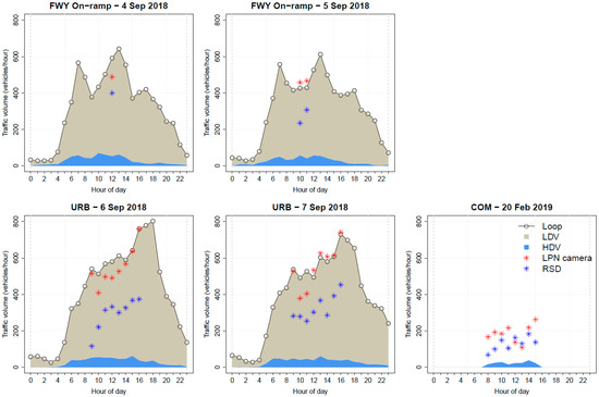
Figure 2.
Traffic count results at three sites using three types of equipment.
Figure 2 shows that count data from the LPN camera using automated image processing are generally comparable with the hourly loop counts, with an average capture rate of 95% (standard deviation ± 11%). The count data using RSD images is generally lower with an average capture rate of 90% (standard deviation ± 14%). This suggests that the LPN camera tends to capture most on-road vehicles and can potentially be used as an alternative (classified) vehicle count device, after proper post-processing of the raw data. This may be a suitable option in the absence of loop detectors, which are relatively expensive to install and operate.
This approach was chosen for the commercial road site where loop detectors were not installed. The LPN and RSD camera data indicate a relatively constant traffic volume during the measurement period, with an average value of 186 and 130 vehicles per hour, respectively.
Note that Figure 2 shows the results for all unique vehicle images for the LPN camera, whereas the RSD data shows the count data for valid RSD measurements only (7889 out of 13,011 measurements). The count results for the RSD give an indication of the proportion of valid vehicle emission measurements within a particular hour. There is significant variability, as can be seen in Figure 2. On average the actual capture rate, expressed as the proportion of total hourly vehicle counts, is 55%. This is lower than 61% expressed as proportion of the total number of RSD samples. Figure 2 shows that the actual capture rate exhibits a significant hourly variation between 21% and 72%.
3.6. Speed and Acceleration
Speed and acceleration data are relevant as they are used to compute vehicle specific power (VSP), which is used to determine on-road engine power and describe driving conditions. VSP is expressed as kW/ton and is computed using the following equation [10]
the variables ν, a, and g represent vehicle speed (m/s), acceleration (m/s2) and gradient (rise/run).
VSP = 1.1 ν a + 9.81 ν g + 0.213 ν + 0.000305 ν 3
Figure 3 shows the speed and acceleration distributions measured by both loop detectors and RSD. The two-sample Kolmogorov-Smirnov test computes p values < 0.001 for both the speed and acceleration distributions, which confirms that the distributions measured with the RSD and loop detectors are significantly different. The measured average speed and average positive acceleration are 27 km/h and +1.8 m/s2 (RSD) and 31 km/h and +0.2 m/s2 (loops), respectively. The acceleration distributions suggest rather constant speed driving.
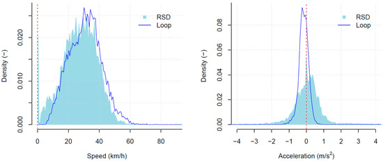
Figure 3.
Comparison of remote sensing devices (RSDs) and loop detector speed and acceleration data.
RSD speeds vary between 0 and 90 km/h and have a larger range compared with the loop detector data (6–69 km/h). The difference is (partly) explained with the short distance of the RSD speed-acceleration bar (0.9 m) versus the longer distance loop detector distances (30–40 m). For a travel speed of 50 km/h, it will take a vehicle about 0.05 s to pass the RSD bar and 2–3 s to pass the loop detectors, providing longer averaging times (and hence reduced variability) in the loop speed measurements.
Nevertheless, RSD speeds exceeding 70 km/h appear unrealistic for this urban site with a speed limit of 60 km/h, and indeed these speeds are flagged as invalid by the RSD. A small portion (2%) of the RSD measurements are recorded as zero speed and are also flagged as invalid, whereas the loop detectors report vehicle speeds between 10 and 54 km/h for these vehicles. The left chart in Figure 3 suggests there is tendency for the RSD to report speeds that are too low, which will affect the accuracy of VSP estimates.
The RSD reports extreme and unrealistic accelerations varying from −110 m/s2 to +138 m/s2, which are flagged as invalid by the RSD. Valid RSD accelerations vary between −6.0 and +4.4 m/s2, whereas the loop detectors have a much narrower range and vary between −1.4 and +1.9 m/s2, as is shown in Figure 3. Note that the acceleration axis range in Figure 3 is capped at ±4 m/s2 for readability purposes, and that 5% of the RSD data are not shown as a result.
It is clear that the use of loop detector speed and acceleration data instead of RSD data will lead to substantially different VSP estimates. In this paper the VSP values provided by the RSD have been used. However, in future papers the impact of loop detector data on the analysis results will be explored.
3.7. High Emitter Detection
Vehicle fleet emissions are dominated by a small percentage of ‘high-emitters’ with excessive emission levels. This has been confirmed by laboratory test programs [11], remote sensing studies [12] and tunnel studies [13]. This skewness in emission distributions is—at least to some extent—due to the variability in emission profiles by vehicle type, the progressive introduction of cleaner engine, and catalyst technology into the vehicle fleet and ageing effects of the in-use fleet.
The skewness of emission distributions for CO, hydrocarbons (HC), and NOx as measured with RSD has increased over the last decade [14], whereas fleet-averaged emissions have decreased considerably. Bishop et al. [15] noted that 1% of on-road vehicles in the USA contributed about 10% to total vehicle emissions in the late 1980s and that this contribution of 1% of on-road vehicles now has increased to about 30%. This change in on-road emission profiles reflects two main trends: (1) the penetration of cleaner vehicles into the fleet over time due to increasingly strict emission standards and improved control technologies with emissions behavior that is characterized with generally low emission levels and brief and large emission peaks; and (2) the presence of vehicles that have excessive emissions, for example due to engine issues, malfunctioning or partly functioning emission control systems, incorrect repairs, lack of servicing and maintenance, poorly retrofitted fuel systems or even tampering.
Remote sensing has been used as a roadside real-time vehicle emissions information system to identify these high-emitting vehicles [16,17]. High emitters are considered to be outliers or anomalies in a statistical sense, i.e., observations with characteristics that are identified to be distinctly different from the other observations. Outliers can be determined in various ways e.g., through examination of univariate and multivariate distributions and at different scales.
Outliers are observations that fall at the outer ranges of the distributions. Observations may occur normally in the outer ranges of a distribution, so this study made an attempt to identify the truly distinctive observations and designate them as anomalies. Outliers can be detected using ‘standard z-scores’. A z-score represents the difference between the observation and the mean in terms of the number of standard deviations. The z-score is negative when the observation is below the mean and positive when above.
There is, however, one issue with this approach. Vehicle emissions are highly skewed with long tails to the right, reflecting occasional emission spikes. Outlier detection using z-scores assumes an (approximate) normal distribution. As a consequence, RSD emissions data need to be transformed before outlier detection can be applied. The aim is to achieve an approximately symmetrical and normal distribution of observed emission rates.
The Box-Cox procedure (R boxcoxfit function) has been used to automatically select the best data transformation from a family of power transformations. Since power transformations require all values to be positive, this procedure includes the option for an automatic location shift. The transformed data z-scores are computed for each combination of vehicle category and pollutant ratio as follows:
where xi is the vehicle-specific RSD observation i, zi is the (transformed) z-score for observation xi, λ is the power transformation parameter, γ is the location shift parameter required, µ* and σ* are the mean, and standard deviation of the transformed data sample, respectively. The z-scores are standardized such that their mean is equal to 0 and standard deviation equal to 1. The two-sample Kolmogorov-Smirnov test is used to test if the (transformed) z-scores have achieved a normal distribution (p > 0.05). Z-score values larger than 3.5, implying that the transformed data value is 3.5 standard deviations (σ*) away from the mean, are considered to qualify as an anomaly and are identified as a high emitter, if pollutant ratios are larger than the mean value.
Figure 4 visualizes the approach. The top left chart shows the observed emissions distribution (n = 51), and the top right chart shows the same distribution after data transformation using λ = 0.2. To verify normality of the transformed distribution, the bottom plots show a quantile-quantile (QQ)-plot (left) and empirical cumulative distribution function (ECDF) plot (right). The ECDF plot graphically shows the probability that the z-score takes a value of less than or equal to X. The x-axis presents the allowable domain for the probability function. Since the y-axis represents probability, it must fall between zero and one. It increases from zero to one as we go from left to right on the horizontal axis.
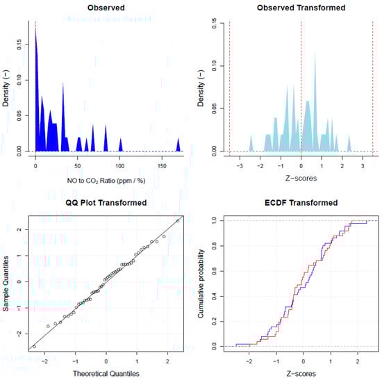
Figure 4.
Example (petrol Euro 2 LCV): transforming NO emission distributions for outlier. ECDF: empirical cumulative distribution function.
The Kolmogorov–Smirnov (KS) test p-value is 0.98, which confirms that the transformed distribution of z-scores (blue line) is not significantly different from a normal distribution (red line). No observations with z-scores larger than 3.5 σ* were found for this particular vehicle category and pollutant, implying there were no high emitters in this sample.
For the full (enhanced) dataset (n = 8991 vehicles), 52 high emitters (0.6%) were identified with the method described in this section. The 3.5 σ* criterion can be relaxed to identify more outliers and high emitting vehicles. However, it should be considered that several vehicles can have high emissions while still being part of the natural distribution of emissions of the on-road fleet for the same technology class. The objective is to identify emission anomalies, i.e., vehicles with excessive emission levels due to technological issues (including tampering) which could potentially be addressed through inspection and maintenance programs, for example.
It is noted that classification for anomaly testing can be refined further and include VSP bins, in addition to vehicle category and pollutant, but that this would require a larger database than used in this study. As an intermediate solution, identified anomalies with high VSP values ≥ 40 kW/ton could be removed, considering that high speed/acceleration conditions are likely to cause high emission levels. The 52 identified vehicles had low to moderate VSP values between −12 and +16 kW/ton.
3.8. High Emitters in Cold Start Mode
Vehicles may have excessive emissions due to technical issues with the engine or emission control system. However, cold starts also lead to short periods with high emissions.
Vehicle emissions are significantly elevated in cold start conditions and are particularly relevant in cold climates. At initial start-up the vehicle engine and emission control systems are cold (ambient temperature), which means more fuel is required and emission control efficiency is reduced and often very low. In contrast, stabilized and low emission hot running conditions occur when the vehicle engine, transmission and emission control technologies have reached their optimal operating temperatures (e.g., engine coolant 75–90 °C, catalysts > 200–250 °C). For instance, in hot running and real-world conditions, three-way catalysts are very effective in reducing engine-out emissions of CO, HC, (organic) PM, and NOx substantially (emission reduction efficiency > 90%). As a consequence, reduced catalyst efficiency due to cold starts has a large impact on vehicle emission levels.
There are different factors that contribute to cold start emissions and they differ in magnitude and duration of impact. Elevated fuel consumption and air pollutant emissions in cold start conditions are due to (1) reduced catalyst efficiency, (2) fuel enrichment in the engine combustion process, and (3) lower fuel efficiency due to increased frictional losses in the engine and transmission systems. The literature suggests that, at an ambient temperature of about 20 °C, hot running conditions should generally be achieved for all relevant vehicle components (engine, transmission, catalyst) within 15 min of driving. However, ‘light-off’ conditions for the catalyst and tight control of the air-to-fuel ratio, which together largely determine the magnitude of cold start emissions, will be achieved much faster than this, i.e., typically within a minute of engine start for modern vehicles and a maximum of a few minutes for older technology vehicles [18].
It is thus important to identify true high emitters with technological issues, and not incorrectly identify vehicles in cold start mode. It is, however, challenging to accurately determine if a vehicle is in cold start mode in real-world driving conditions. In local emission (remote sensing) testing programs it is generally (and often incorrectly) assumed that cold start emissions are not significant and can be ignored [5].
Few researchers have attempted to determine which specific vehicles operate in cold start mode. Monateri et al. [19] reported on the (manual) use of an infrared (IR) camera to measure the heat signature of passing vehicles (exhaust, tires, and underbody) and determine if a vehicle is in cold start mode.
Smit and Kingston [7] developed, tested, and used two independent methods to identify vehicles operating in cold start mode. The first method assessed the likelihood that a particular measurement site is impacted by cold start vehicles by tracking the journeys of individual vehicles using a network of Bluetooth monitoring units at and around each measurement site. The second method analyzed the thermal IR signatures of individual vehicles to identify those in cold start conditions and is used in this study. A special test program [7] showed that the thermal signature of cold start vehicles is dark for the first 1–2 min after engine start. After about 2 min of driving, the thermal signature of the vehicle becomes visible. The IR signature has various components that light up varying from the exhaust system, tires/brakes, and the thermal reflection that radiates from the underbody. The tires/brakes and exhaust pipe (if visible) in particular appear to be good indicators for driving in cold start conditions. Hot vehicles exhibit hot and clearly distinguishable wheels/brakes and exhaust systems, and regularly an intense and bright reflection off the road surface. In contrast, cold vehicles will generally appear to be dark and have the same or only slightly brighter IR reflection on the road.
After identification of the 52 high-emitters, date-time stamped heat signature images were retrieved for analysis. The thermal images were then used to visually assess if a high emitting vehicle is (likely) producing high emissions due to cold start conditions. Figure 5 (next page) shows an example of two Euro 5 diesel LCVs that were identified as high emitters for CO but were assessed differently as either a hot or a cold start vehicle.
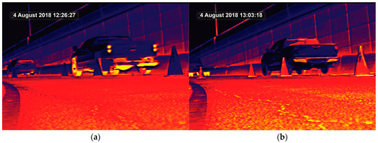
Figure 5.
Examples of heat signature images of two vehicles, one assessed as being a ‘hot high emitter’ (a) and one as a ‘cold start high emitter’ (b).
The total sample size for this vehicle category (diesel Euro 5 LCV) is 870 vehicles. The vehicle assessed as a cold start high emitter ranked as number 1 and had the highest z-score (4.3) and highest recorded CO/CO2 ratio (0.11%/%). The vehicle assessed as a hot high emitter ranked a number 5 and had a z-score of 3.9 and a recorded CO/CO2 ratio of 0.04%/%. Approximately 35% of the 52 identified high emitters were assessed to be in cold start mode based on their thermal signature.
This implies that, in areas where a significant number of cold start vehicles are likely (e.g., urban areas), a substantial portion of high emitting vehicles are potentially incorrectly identified by an RSD as vehicles that require enhancements to significantly reduce emissions. The additional use of a thermal camera can then help to address this issue. If a thermal camera is not available for an RSD campaign, an initial screening criterion for potential cold start mode interference could be a minimum distance between residential address (if know from vehicle registration data) and RSD sampling site of at least a few kilometers.
It is finally noted that the number of high-emitters in the on-road fleet is typically small and that their emissions are highly variable, more so than properly functioning vehicles [20]. In terms of identifying high emitters and consideration of this variability, identification of the same vehicle at multiple dates/times appears sensible before the owner is contacted and instructed to have the vehicle repaired.
3.9. RSD Data Analysis: Trends in Vehicle NOx Emissions
The RSD reports concentration levels in the exhaust gas, i.e., CO2 (%), CO (%), HC (ppm), and NO (ppm), corrected for water and excess oxygen not used in the combustion process. However, the exhaust plume path length and the density of the observed plume are highly variable from vehicle to vehicle and are a function of the height of the vehicle’s exhaust pipe, wind direction and speed, and turbulence behind the vehicle, amongst other factors. The RSD can therefore only reliably measure ratios of CO, HC, and NO to CO2. These ratios are assumed to be constant in a particular vehicle’s exhaust plume. Due to the short time period involved in the measurement, this is expected to hold true for reactive species such as NO as well. However, RSD data are naturally noisy and sufficiently large sample sizes are required to obtain significant results.
Overseas studies have demonstrated poor real-world NOx performance of diesel passenger cars, which have contributed to persistent NO2 air quality issues in many EU cities [21,22]. NOx emission rates from diesel cars have not significantly reduced over progressive Euro standards [23]. They have also undergone a significant shift towards higher primary NO2 to NOx ratios, mainly due to implementation of more effective PM emission control technologies, such as (combined) diesel oxidation catalysts and catalyzed particulate filters. These mean ratios have changed from about 15% for pre-Euro technology to almost 60% for Euro 4–6 technology cars, although ratios as high as almost 80% have been reported [4,24,25,26,27].
Primary NO2-to-NOx ratios are critically dependent on type of emission control technology used, which explains the large observed variability in measured ratios [28,29]. In addition, there is some evidence that larger (diesel) cars have higher NO2 emission rates [30] and that NO2-to-NOx ratios are reduced as vehicles age [31].
It is therefore of interest to examine if the same behavior is observed in the Australian RSD data. This is particularly relevant now as the Australian on-road fleet has experienced a strong increase in the sale of large diesel cars (SUVs) [32]. In addition, the current Australian (Euro 5 equivalent) emission standards are likely to be in place until 2027, at which time Euro 6 standards will likely be introduced.
Although NO2 measurement has recently become a feature of remote sensing [30], remote sensing studies have traditionally used RSDs that measure NO only, as is the case in this study. In contrast, on-road or laboratory measurements, as well as emission factors used in vehicle emission predictions, relate to the sum of NO and NO2 (i.e., NOx, expressed as NO2 equivalents). Direct use of NO data from RSD would therefore result in an underestimation (bias) of RSD NOx emission rates. For petrol vehicles this a less significant issue as petrol cars exhibit low NO2/NOx shares in the order of 5%, which are approximately independent of emissions standard.
Therefore, a suitable adjustment factor is required to convert measured RSD NO data to an estimate of NOx-to-CO2 ratios and properly account for primary NO2 emissions. The NOx-to-CO2 ratio is computed using the vehicle technology dependent mass fraction of NO2 in vehicle exhaust (fNO2). Table 2 shows the reported fNO2 ranges in the literature and the selected fNO2 value for each vehicle type and Euro class. The NOx-to-CO2 ratio is computed as NO/(1-fNO2), where NO is the measured RSD NO-to-CO2 concentration ratio (ppbv/%).
Table 2.
NO2 to NOx ratios: reported ranges * and selected values for this study.
The RSD data were classified by vehicle category (e.g., vehicle type, fuel type, euro standard) and vehicle specific power (VSP). VSP normalizes RSD data for ‘driving conditions’ and is commonly used as an explanatory variable in emission simulation, particularly in the USA [33]. VSP (kW) is calculated by the RSD using speed and acceleration for each individual vehicle. Six VSP bins were used to classify the data. They are defined as VSP < 0 kW/(metric) ton, 0 ≤ VSP < 5 kW/ton, 5 ≤ VSP < 10 kW/ton, 10 ≤ VSP < 20 kW/ton, 20 ≤ VSP < 40 kW/ton, and VSP ≥ 40 kW/ton. It is noted that other researchers have used a larger number of VSP bins, e.g., 14 bins [34] and 2 kW/ton bins [30]. However, NIWA [5] found that the difference between a 6 or 14 bin classification is not statistically significant when the variability in the RSD emissions data is considered. The six bins and their boundaries use a logical distinction in driving behavior and generally ensure a sufficient sample sizes for each bin [4].
Figure 6 shows the comparison of NOx-to-CO2 ratios for petrol and diesel cars, SUVs and LCVs. Colored bars reflect measured data and color intensity is used to show the sample size for each VSP-Euro class bin. The estimated NO2 portion is shown in grey. Single vehicle measurements (n = 1) were removed and are not presented. It is noted that Australian emissions legislation did not adopt Euro 3 for diesel LDVs; therefore, it is not included in Figure 6.
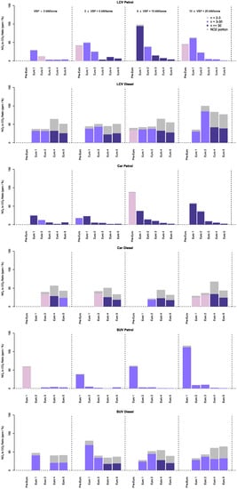
Figure 6.
Mean NOx-to-CO2 ratios for petrol and diesel light duty vehicles (LDVs) by vehicle type and VSP/Euro class.
Figure 6 shows a consistent pattern of reduction in NOx-to-CO2 ratios for petrol LDVs across all VSP bins, with more recent technology vehicles (Euro 3+) exhibiting relatively low NOx emissions. In contrast, diesel LDVs generally show stabilizing or even increasing NOx-to-CO2 ratios, which confirms that the NOx emission issues with diesel vehicles in Europe are similarly observed in Australia.
The difference in real-world CO2 emissions between petrol and diesel cars has become smaller over time with Euro 1 diesel LDVs emitting about 5% less CO2 per km of driving, reducing to a negligible difference for Euro 5(+) LDVs [35]. Accounting for the difference in CO2 emissions, it is clear that the gap in real-world NOx emissions between diesel and petrol LDVs has increased substantially with progressive emission standards. The ratio of diesel to petrol NOx emissions for Euro 2 technology was about 0.6–0.7, which means that diesel LDVs had, on average, approximately 30–40% lower NOx emissions than petrol LDVs.
However, for Euro 4 and 5 technology the picture is very different. Euro 4 diesel LDVs emit approximately a factor of 10 (LCVs), 16 (cars) and 27 (SUVs) more NOx per km than the corresponding petrol LDVs. Euro 5 diesel LDVs emit approximately a factor of 15 (LCVs), 12 (cars) and 23 (SUVs) more NOx per km than the corresponding petrol LDVs.
The evidence suggests that Australia is potentially heading for local air quality issues near roads that are similar to Europe, due to a combination of compounding factors. First, this study confirms poor NOx emissions performance of Euro 4 and 5 diesel LDVs in Australia, which is in line with extensive research regarding the European on-road fleet. Second, the issue is compounded by a continued and strong increase in LDV dieselization of the Australian fleet and SUV sales. Third, there is no (clear) plan to implement Euro 6 emission standards in Australia, which means that the sale of Euro 5 technology LDVs is allowed to continue, potentially until 2027. These factors combined will lead to an increasing proportion of high-NOx emission vehicles in the on-road fleet. Fourth, Australia will likely adopt significantly more stringent NO2 air quality criteria in 2020 and 2025, potentially surpassing current EU criteria. At this stage it is proposed that the current NO2 criterion (annual) of 62 µg/m3 will reduced to 39 and 31 µg/m3 in 2020 and 2025, respectively, a reduction of 37% and 50%. The current annual EU air quality standard is 40 µg/m3. The short term NO2 criterion (99.7P) of 250 µg/m3 is also proposed to be reduced to 185 and 164 µg/m3 in 2020 and 2025, respectively, a reduction of 26% and 34%. The current short-term EU air quality standard (99.8P) is 200 µg/m3. This development increases the risk of local air quality exceedances near busy roads.
4. Conclusions
This paper discussed and presented selected results from a short but comprehensive on-road emission measurement program conducted in Brisbane, Australia. The study used and combined a range of instruments that measured vehicle emissions (on-road and dynamometer), on-road air quality, traffic activity and performance at the measurement sites, vehicle journeys in the vicinity of the sites (vehicle tracking), on-road vehicle thermal profiles, and license plate recognition.
The results show that supplementing RSD equipment with additional equipment can generate certain benefits; it can significantly increase sample size (e.g., LPN camera, loop detectors) and provide useful new information that assists in the analysis of on-road emissions data (e.g., thermal imaging camera, MAC address units, loop detectors).
Use of the second LPN camera and loop detectors increased RSD capture rate with almost 10% and may reduce bias in RSD measurements by better capturing older dirtier and/or smoky vehicles. The second camera can also be used as a cheap and independent vehicle count device. Post-processing of data from both the LPN camera and loop detectors is required to obtain useful and accurate information.
This paper has presented a method to identify vehicles with excessive emission levels (high emitters), as measured with the remote sensing device (RSD). The first step is to apply an anomaly detection method based on a statistical data transformation and standardization technique. Using this method, 0.6% of the vehicles in the full (enhanced) RSD dataset (n = 8991 vehicles) were identified as high emitters. The second step was to examine thermal profiles for the identified vehicles to assess if measured high emission levels could be caused, at least to some extent, by cold start operating conditions. A special test program was conducted to associate key factors in a thermal profile (e.g., tires/brakes, exhaust pipe, underbody) with time since engine start. Analysis of the thermal IR signatures of the individual vehicles showed that approximately 35% of the high emitters are likely in cold start mode. This implies that, in areas where a significant number of cold start vehicles are likely (e.g., urban areas), a substantial portion of high emitting vehicles are potentially incorrectly identified by an RSD as vehicles that require enhancements to significantly reduce emissions. The additional use of a thermal camera can then help to address this issue.
Analysis of NOx RSD data confirms that poor real-world NOx performance of Euro 4/5 diesel passenger cars and LCVs observed around the world is also evident in the Australian measurements. The evidence suggest that Australia is potentially heading for local air quality issues near busy roads, similar to Europe, due to a combination of compounding factors. These compounding factors are a continued and strong increase in LDV dieselization of the Australian fleet, no (clear) plan to implement Euro 6 emission standards in Australia, and adoption of significantly more stringent NO2 air quality criteria in Australia in 2020 and 2025, potentially surpassing current EU criteria.
The data used in this study was generated in a short but intensive measurement campaign. It would be interesting to see if the findings in this study are confirmed in other (larger) programs. In particular the use of thermal profiling in combination with high emitter detection could be further tested and explored. The feasibility of full automation of this process can be further explored. A limitation of this study is that NO2 emissions had to be estimated as the RSD we used did not include NO2 measurement.
Author Contributions
Conceptualization, R.S.; methodology, R.S.; formal analysis, R.S.; investigation, R.S.; writing—original draft preparation, R.S. and P.K.; writing, R.S., visualization, R.S. and P.K.; supervision, R.S.; project administration, R.S. and P.K.
Funding
This research received no external funding.
Acknowledgments
The authors are grateful for the help provided by Scott Bainbridge of the Western Australia Department of Water and Environmental Regulation (WA DWER, Australia), Barbara Downs and Abbie Brooke of Brisbane City Council (Australia), Elizabeth Somervell of NIWA (New Zealand) and Ray Wilson of the Department of Transport and Main Roads (DTMR, Australia). WA DER is acknowledged for kindly loaning the RSD equipment to the Department of Environment and Science (DES) for 6 months. DTMR is acknowledged for kindly loaning the thermal imaging camera to DES. The technical support from the DES air quality monitoring team is appreciated and acknowledged.
Conflicts of Interest
The authors declare no conflict of interest.
References
- Caiazzo, F.; Ashok, A.; Waitz, I.A.; Yim, S.H.L.; Barrett, S.R.H. Air pollution and early deaths in the United States. Part I: Quantifying the impact of major sectors in 2005. Atmos. Environ. 2013, 79, 198–208. [Google Scholar] [CrossRef]
- Smit, R.; Brown, A.L.; Chan, Y.C. Do air pollution emissions and fuel consumption models for roadways include the effects of congestion in the roadway traffic flow? Environ. Modell. Softw. 2008, 23, 1262–1270. [Google Scholar] [CrossRef]
- Smit, R.; Ntziachristos, L.; Boulter, P. Validation of road vehicle and traffic emission models—A review and meta-analysis. Atmos. Environ. 2010, 44, 2943–2953. [Google Scholar] [CrossRef]
- Smit, R.; Bluett, J. A new method to compare vehicle emissions measured by remote sensing and laboratory testing: High-emitters and potential implications for emission inventories. Sci. Total Environ. 2011, 409, 2626–2634. [Google Scholar] [CrossRef] [PubMed]
- Smit, R.; Somervell, E. The Use of Remote Sensing to Enhance Motor Vehicle Emission Modelling in New Zealand; National Institute of Water & Atmospheric Research: Auckland, New Zealand, 2015. [Google Scholar]
- ESP. RSD4600 NextGen Operator’s Manual, 2nd ed.; Environmental Systems Products Holdings Inc.: Tucson, AZ, USA, 2006. [Google Scholar]
- Smit, R.; Kingston, P. Detecting cold start vehicles in the on-road fleet. Air Qual. Clim. Chang. 2019, 53, 22–26. [Google Scholar]
- Smit, R.; Kingston, P.; Neale, D.W.; Brown, M.K.; Verran, B.; Nolan, T. Monitoring on-road air quality and measuring vehicle emissions with remote sensing in an urban area. Atmos. Environ. 2019, in press. [Google Scholar]
- ALPR. Automated License Plate Recognition. Available online: https://github.com/openalpr/openalpr (accessed on 9 October 2018).
- Kuhns, H.D.; Mazzoleni, C.; Moosmuller, H.; Nikolic, D.; Keislar, R.E.; Barber, P.W.; Li, Z.; Etyemezian, V.; Watson, J.G. Remote sensing of PM, NO, CO and HC emission factors for on-road gasoline and diesel engine vehicles in Las Vegas, NV. Sci. Total Environ. 2004, 322, 123–137. [Google Scholar] [CrossRef] [PubMed]
- Choo, S.; Shafizadeh, K.; Niemeier, D. The development of a prescreening model to identify failed and gross polluting vehicles. Transpn Res. D 2007, 12, 208–218. [Google Scholar] [CrossRef][Green Version]
- Zhang, Y.Z.; Stedman, D.H.; Bishop, G.A.; Guenther, P.L.; Beaton, S.P. Worldwide on-road vehicle exhaust emissions study by remote sensing. Environ. Sci. Technol. 1995, 29, 2286–2294. [Google Scholar] [CrossRef] [PubMed]
- Smit, R.; Kingston, P.; Wainwright, D.; Tooker, R. A tunnel study to validate motor vehicle emission prediction software in Australia. Atmos. Environ. 2017, 151, 188–199. [Google Scholar] [CrossRef]
- Park, S.S.; Kozawa, K.; Fruin, S.; Mara, S.; Hsu, Y.K.; Jakober, C.; Winer, A.; Herner, J. Emission factors for high-emitting vehicles based on on-road measurements of individual vehicle exhaust with a mobile measurement platform. J. Air Waste Manag. Assoc. 2012, 61, 1046–1056. [Google Scholar] [CrossRef]
- Bishop, G.A.; Schuchmann, B.G.; Stedman, D.H.; Lawson, D.R. Multispecies remote sensing measurements of vehicle emissions on Sherman Way in Van Nuys, California. J. Air Waste Manag. Assoc. 2012, 62, 1127–1133. [Google Scholar] [CrossRef]
- Sjödin, Å.; Andréasson, K.; Wallin, M.; Lenner, M.; Wilhelmsson, H. Identification of high-emitting catalyst cars on the road by means of remote sensing. Int. J. Vehicle. Des. 1997, 18, 326–339. [Google Scholar]
- Bishop, G.A.; Stedman, D.H. A decade of on-road emissions measurements. Environ. Sci. Technol. 2008, 42, 1651–1656. [Google Scholar] [CrossRef] [PubMed]
- Smit, R.; Ntziachristos, L. Cold start emission modelling for the Australian petrol fleet. Air Qual. Clim. Chang. 2013, 47, 31. [Google Scholar]
- Monateri, A.M.; Stedman, D.H.; Bishop, G.A. Infrared thermal imaging of automobiles. In Proceedings of the 14th CRC On-Road Vehicle Emissions Workshop, San Diego, CA, USA, 21 March–2 April 2004. [Google Scholar]
- Schulz, D.; Younglove, T.; Barth, M. Statistical Analysis and Model Validation of Automobile Emissions; Research and Innovative Technology Administration: Washington, DC, USA, 2000. [Google Scholar]
- Carslaw, D.C.; Beevers, S.D.; Tate, J.E.; Westmoreland, E.J.; Williams, M.L. Recent evidence concerning higher NOx emissions from passenger cars and light duty vehicles. Atmos. Environ. 2011, 45, 7053–7063. [Google Scholar] [CrossRef]
- Beevers, S.D.; Westmoreland, E.; De Jong, M.C.; Williams, M.L.; Carslaw, D.C. Trends in NOx and NO2 emissions from road traffic in Great Britain. Atmos. Environ. 2012, 54, 107–116. [Google Scholar] [CrossRef]
- Borken-Kleefeld, J.; Dallmann, T. Remote Sensing for Motor Vehicle Exhaust Emissions; The International Council on Clean Transportation (ICCT): Washington, DC, USA, 2018. [Google Scholar]
- Gense, R.; Vermeulen, R.; Weilenmann, M.; McCrae, I. NO2 emissions from passenger cars. In Proceedings of the 2nd Conference on Environment and Transport, Reims, France, 12–14 June 2006. [Google Scholar]
- Grice, A.; Stedman, J.; Kent, A.; Hobson, M.; Norris, J.; Abbott, J.; Cooke, S. Recent trends and projections of primary NO2 emissions in Europe. Atmos. Environ. 2009, 43, 2154–2167. [Google Scholar] [CrossRef]
- Rhys-Tyler, G.A.; Bell, M.C. Toward reconciling instantaneous roadside measurements of light-duty vehicle exhaust emissions with type approval drive cycles. Environ. Sci. Technol. 2012, 46, 10532–10538. [Google Scholar] [CrossRef]
- Carslaw, D.C.; Rhys-Tyler, G. New insights from comprehensive on-road measurements of NOx, NO2 and NH3 from vehicle emission remote sensing in London, UK. Atmos. Environ. 2013, 81, 339–347. [Google Scholar] [CrossRef]
- Kousoulidou, M.; Ntziachristos, L.; Mellios, G.; Samaras, Z. Road-transport emission projections to 2020 in European urban environments. Atmos. Environ. 2008, 42, 7465–7475. [Google Scholar] [CrossRef]
- EMEP/EEA Emission Inventory Guidebook 2016; European Environment Agency (EEA): Copenhagen, Denmark, 2016.
- Borken-Kleefeld, J.; Hausberger, S.; McClintock, P.; Tate, J.; Carslaw, D.; Bernard, Y.; Sjödin, Å. Comparing Emission Rates Derived from Remote Sensing with PEMS and Chassis Dynamometer Tests–CONOX Task 1 Report; IVL Swedish Environmental Research Institute, Commissioned by Federal Office for the Environment: Stockholm, Switzerland, 2018; ISBN 978-91-88787-28-6. [Google Scholar]
- Carslaw, D.C.; Murrells, T.P.; Andersson, J.; Keenan, M. Have vehicle emissions of primary NO2 peaked? Faraday Discuss. 2016, 189, 439–454. [Google Scholar] [CrossRef] [PubMed]
- ABS. Survey of Motor Vehicle Use, Australian Bureau of Statistics. Available online: www.abs.gov.au (accessed on 12 March 2019).
- International Vehicle Emissions Model. Available online: http://www.issrc.org/ive/ (accessed on 7 February 2019).
- Frey, H.C.; Unal, A.; Chen, J.; Li, S. Evaluation and recommendation of a modal method for modelling vehicle emissions. In Proceedings of the 12th International Emission Inventory Conference—“Emission Inventories-Applying New Technologies”, San Diego, CA, USA, 29 April–1 May 2003. [Google Scholar]
- Helmers, E.; Leitao, J.; Tietge, U.; Butler, T. CO2-equivalent emissions from European passenger vehicles in the years 1995–2015 based on real-world use: Assessing the climate benefit of the European “diesel boom”. Atmos. Environ. 2019, 198, 122–132. [Google Scholar] [CrossRef]


© 2019 by the authors. Licensee MDPI, Basel, Switzerland. This article is an open access article distributed under the terms and conditions of the Creative Commons Attribution (CC BY) license (http://creativecommons.org/licenses/by/4.0/).