Quantitative Detection of Dust Storms with the Millimeter Wave Radar in the Taklimakan Desert

Abstract

In order to conduct real-time quantitative monitoring of dust storms, Ka-band millimeter wave radar (MMWR) was utilized for the consecutive detection of dust storms over the Taklimakan Desert from April to June 2018. The retrievals of the reflectivity factor, dust spectrum distribution and dust mass concentration were carried out with the power spectrum data detected by MMWR for three dust storm processes. The analysis shows that: The probability density distribution of dust conforms to the lognormal distribution. During the dust storm processes, the effective detection height of the reflectivity factor was within 2000 m and the range of the reflectivity factors was between $-25\mathrm{dBZ}$ and $25\mathrm{dBZ}$. During the floating dust period, the effective height of the dust spectrum distribution was lower than 300 m and the values of dust mass concentration were less than 31.62 $\mathsf{\mu }\mathrm{g}·{\mathrm{m}}^{-3}$, at a height of 200 m. Furthermore, during the blowing sand stage, the effective height of the dust spectrum distribution was normally lower than 600 m and the values of dust mass concentration were mainly less than $316.23\mathsf{\mu }\mathrm{g}·{\mathrm{m}}^{-3}$, at a height of 200 m. During the dust storm period, the effective height of the dust spectrum distribution exceeded 1000 m; when the height was 100 m, the values of dust mass concentration were between $1220\mathsf{\mu }\mathrm{g}·{\mathrm{m}}^{-3}\mathrm{and}\mathrm{42,146}\mathsf{\mu }\mathrm{g}·{\mathrm{m}}^{-3}$ and the average mass concentration was $9287\mathsf{\mu }\mathrm{g}·{\mathrm{m}}^{-3}$; whereas, the values of dust mass concentration were between $2\mathsf{\mu }\mathrm{g}·{\mathrm{m}}^{-3}\mathrm{and}820\mathsf{\mu }\mathrm{g}·{\mathrm{m}}^{-3}$ when the height was 1200 m and the average mass concentration was $24\mathsf{\mu }\mathrm{g}·{\mathrm{m}}^{-3}$. The relationship between the reflectivity factor Z and the dust mass concentration M is defined as $Z=651.6M^{0.796}$. Compared with the observational data from Grimm180 particle detector, the data of the retrieved dust mass concentration are basically accurate and this retrieved method proves to be feasible. Thus, the MMWR cans be used as a new device for quantitative monitoring of dust storms.

1. Introduction

Dust storms are a disastrous natural phenomenon, which can cause serious damage to human habitats, including breaking down industrial machinery, disrupting traffic, harming vegetation and deteriorating air quality [1,2,3,4,5]. High dust loading in the air due to the dust storms could also impact the solar radiation balance, cloud formation, secondary pollutant generation and marine primary productivity, which has a complex influence on the ecosystem [6,7,8]. The impact of a dust storm is not limited to the source areas but extends to larger regional or even global scales [9,10]. Therefore, the quantitative monitoring of dust storms is of great significance for disaster prevention, environmental protection and sustainable development.

Recently, satellite remote sensing and Micro Pulse Lidar (MPL) technologies have been commonly used for monitoring dust storms [11,12,13,14]. For instance, Lei and Wang [15] defined a set of common characteristics for different types of dust storms over the western US based on stationary satellite datasets. Kai et al. [16] studied the structure of dust layer over Taklimakan desert in April 2002 by MPL. Satellite remote sensing technology, which can monitor the coverage and transport routes of dust storms, but it is not able to extract such data as specific vertical structure of dust storm, sand content in the air and sand-dust particle concentrations [17,18,19]. Contrastingly, the MPL technology can observe the vertical structure, composition and optical properties of sand-dust aerosols in real-time. However, owing to the low transmitted power, MPL cannot penetrate the entire profile of strong dust storms [20]. Hence, how to conduct real-time quantitative monitoring of dust storms has always been an unsolved problem. In order to address the problem, the dust storms over the Taklimakan Desert are detected and analyzed in this paper, with the Millimeter Wave Radar (MMWR).

The MMWR has many outstanding features, such as: Millimeter wavelength, a high range resolution, low power consumption and can continuous monitoring and extracting of the vertical reflectivity factor [21]. Because of its wavelength, the MMWR provides robust information even in degraded conditions. It has been used to monitor the height of clouds [22,23], and analyze the clouds’ water [24], precipitation [25] and snow contents [26]. During the dust storm period, the transmitting wave of MMWR is scattered by sand-dust particles, and therefore, generates a scattered echo which can be received by the MMWR receiver [27,28,29]. Juan et al. [30] and Nashashibi et al. [31] analyzed the theory of applications of MMWR for the detection of dust storms. Although the previous studies have proved that the MMWR could be effective in the detection of dust storms in theory, this paper initiates the first long-term continuously quantitative detection of dust storms with the MMWR.

The Taklimakan Desert, the world’s second largest moving sand-dune desert, is one of the regions with a high frequency of dust storms. The dust storms in the Taklimakan Desert, which are associated with active cold fronts, mostly occur in the spring [32,33,34]. Dusts from the Taklimakan, which transport routes along west-central China and the Tibetan Plateau, play an important role in the regional and East Asian climate [35].

In order to study on the quantitative features of dust storms occurring in the Taklimakan Desert, the processes of dust storm events from April to June 2018 are detected and analyzed in this paper, using a Ka-band MMWR. Firstly, the altitudinal-temporal distribution features of reflectivity factors are calculated and analyzed. Secondly, the altitudinal-temporal distributions of dust particle spectrums and dust mass concentrations are retrieved. Finally, the Z (reflectivity factor)-M (dust mass concentration) equation is established to represent the relationship between reflectivity factor and dust mass concentration.

2. Instrumentation and Data

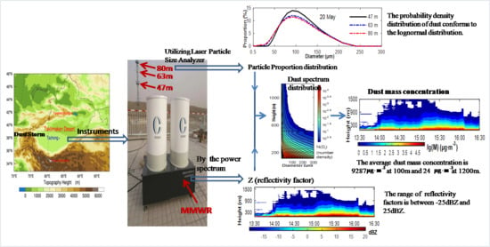
2.1. Site and Instruments

The detection was carried out at Tazhong Experimental Station (39°00′ N, 83°40′ E, 1099.3 m above sea level), which is located in the center of the Taklimakan Desert (see Figure 1b). All year round, the climate of this region is droughty, with little precipitation and is hit by frequent dust storms. The sparsely vegetated region embodies paradigmatic geomorphic features of the Taklimakan Desert.

The main instruments used for detection of dust storms in this study were the Ka-band MMWR, the dust collection instruments, the Laser Particle Size Analyzer (LPSA) and the Grimm180 particle detector.

The Ka-band MMWR is manufactured by Anhui Sichuang Electronics Company (Figure 1a). The MMWR, which has high vertical range resolution (10 m), can generate a set of data per 1 min and its main configuration parameters are shown in

Table 1. Parameters of Ka-band millimeter continuous wave radar.

Parameter Name	Value	Parameter Name	Value
Wavelength	$8.26\mathrm{mm}$	Pulse width	$2560 \mathsf{\mu }\mathrm{s}$
Range resolution	10 m	Transmit power	10 w
Center frequency	35 GHz	FFT points	256
Horizontal beam width	${1.2}^0$	Feeder loss	1.2 dB
Vertical beam width	${1.2}^0$	Antenna gain	40 dB

.

The dust collection instruments were installed at the 47 m, 63 m and 80 m heights of the flux tower which is installed in the hinterland of the Taklimakan Desert (Figure 1a). The dust collection instruments collected the dust particles during every dust storm. The LPSA is manufactured by Everise Technology Ltd. And retrieved particle proportion distributions based on the particle laser scattering principle.

The Grimm180 particle detector, which is made by Grimm Company in Germany, consists of 32 channels. Real-time measurements of the dust mass concentrations with diameters less than $10 \mathsf{\mu }\mathrm{m}$ can be conducted by Grimm180. The consecutive detection of dust storms over the Taklimakan Desert was conducted from April to June 2018 with those instruments.

2.2. Description of Dust Storm Processes

Three strong dust storms occurred over the Taklimakan Desert from April to June 2018. Based on the differences of the visibility and the ground wind speed during the stages of the dust events (Rashki [36,37]; the regulations of China Meteorological Administration): The weather is a dust storm when the ground wind speed is very large and the visibility is less than 1 km; however, when the ground wind speed is relatively large and the visibility is between 1 km and 10 km, the weather is considered as blowing sand, whereas, during floating dust, the ground wind speed is small and the visibility is between 1 km and 10 km.

Table 2. Observation times of the dust storm processes.

Date	Floating Dust	Blowing Sand	Dust Storm
7 May	11:00–11:30; 17:30–19:00	11:30–13:35; 16:00–17:30	13:35–16:00
20 May	13:30–13:40	13:40–14:10; 16:08–16:30	14:10–16:08
24 May	8:50–12:00; 17:20–19:00	12:00–14:20; 17:10–17:20	14:20–17:10

shows the ground observation time for the three dust storm processes. This paper mainly uses the detection data of the three dust storms by the MMWR, the data retrieved by the LPSA and the observational data from Grimm180. Beijing time (BT) is applied in this study and the time of the Figures is displayed from left to right.

3. Method for the Retrieval of Dust Spectrum Distribution

Dust spectrum distribution is the distribution of sand-dust density, varying in terms of different sand-dust particle diameters per unit volume ($1{\mathrm{m}}^3$). The original data used in this paper is the frequency power spectrum data observed by the MMWR. The retrieval method is illustrated with the example of the power spectrum data$\left(S\left({\mathrm{f}}_{\mathrm{i}}\right)\right)$ observed by the MMWR at a height of 100 m at 15:40 on 24 May (Figure 2a).

3.1. The Calculation of the Reflectivity Factor

With the radar meteorological equation (Zhang et al. [38]), the reflectivity factors (Z) can be calculated by the following formula.

$$Z=\frac{1024\times ln2\times {\lambda }^2\times R^2\times L\times P_r}{{\pi }^3\times P_t\times c\times \tau \times G^2\times \phi \times \theta \times {10}^{-0.2{{\displaystyle \int }}_0^{R}k\mathrm{d}R}\times {\left|\frac{m^2-1}{m^2+2}\right|}^2}$$

(1)

where$\mathsf{\lambda }$ is the wave length ($8.26\mathrm{mm}$), R is the target distance, L is the feeder loss (1.2 dB), $P_t$ is the radar transmitting power (10 w), $\mathrm{c}$ is the transmitting speed of the electromagnetic wave ($3\times {10}^8\mathrm{m}·{\mathrm{s}}^{-1}$), $\mathsf{\tau }$ is the pulse width ($2560\mathsf{\mu }\mathrm{s}$), G is the antenna gain (40 dB), $\mathsf{\phi }$ is the horizontal beam width (0.02 rad), $\mathsf{\theta }$ is the vertical beam width (0.02 rad) and ${\left|\frac{m^2-1}{m^2+1}\right|}^2$ is the square of the complex refraction index (0.3).

In Equation (1), the $P_r$ represents the echo power received by the radar, which can be calculated with the power spectrum$\mathrm{S}\left({\mathrm{f}}_{\mathrm{i}}\right)$. The equation is given as:

$$P_r={{\displaystyle \sum }}_1^{\mathrm{N}}\frac{\mathrm{S}\left({\mathrm{f}}_{\mathrm{i}}\right)}{{\mathrm{N}}_{\mathrm{f}}}\times \mathrm{K}\times {\mathrm{T}}_0\times \mathrm{B}$$

(2)

where N is the number of FFT (Fast Fourier Transform) points (256), K is Boltzmann constant ($1.38\times {10}^{-23} \mathrm{J}/\mathrm{K}$), B is the receiver bandwidth (4 MHz), ${\mathrm{T}}_0$ is the radar antenna temperature expressed by absolute temperature (290 K) and${\mathrm{N}}_{\mathrm{f}}$ is the noise factor.

By Equations (1) and (2), the reflectivity factor Z can be obtained by utilizing the power spectrum$\mathrm{S}\left({\mathrm{f}}_{\mathrm{i}}\right)$. The Z calculated by $\mathrm{S}\left({\mathrm{f}}_{\mathrm{i}}\right)$ is $18.97\mathrm{dBZ}$ in Figure 2.

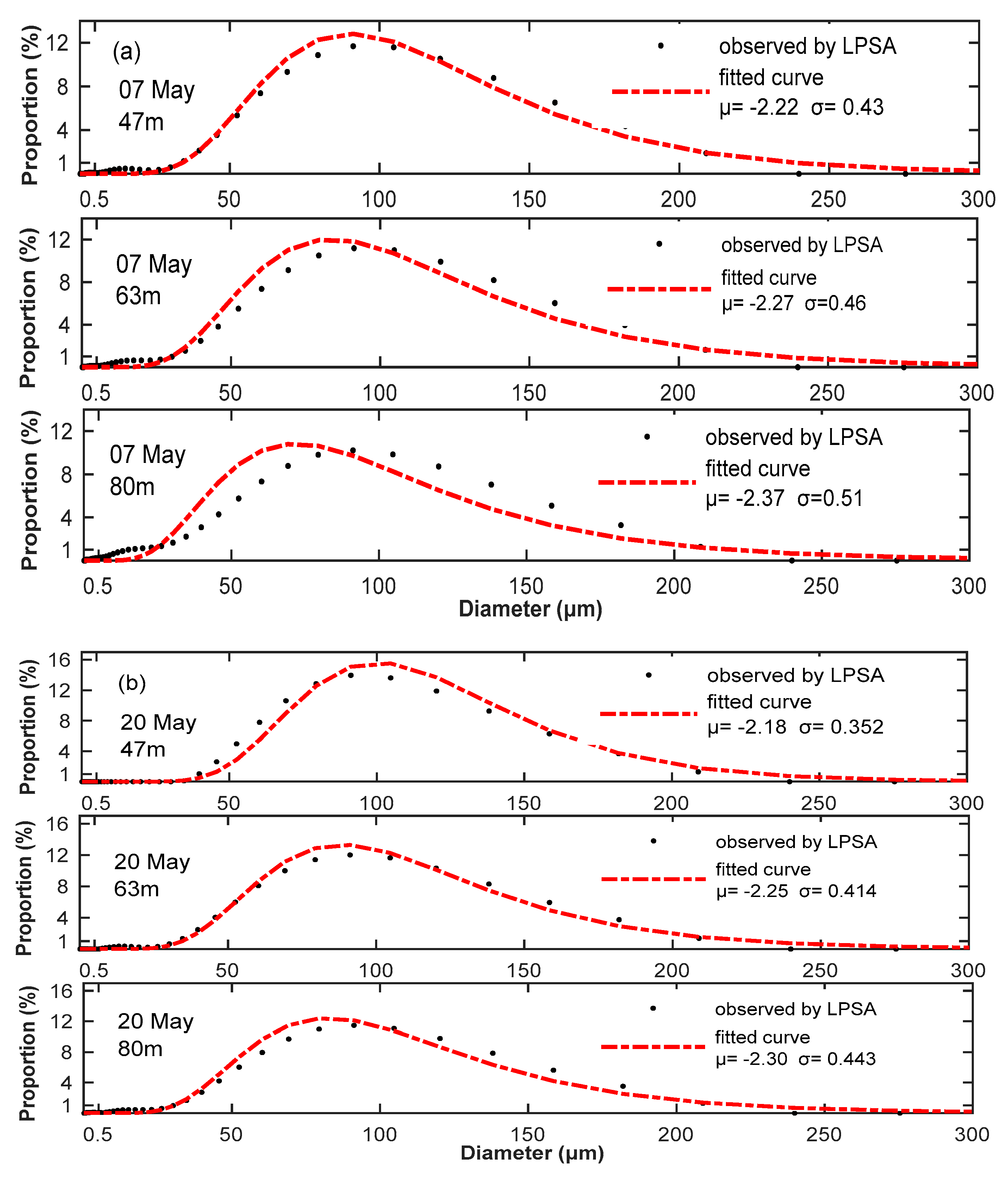
3.2. The Probability Density Distribution of Dust Particles

Firstly, with the LPSA, the particle proportion distributions of the three dust storms are retrieved by analyzing the dust particles collected by the dust collection instruments. Secondly, the particle proportion distributions at the 47 m, 63 m and 80 m heights of the three events are shown in Figure 3. Form the Figure 3, the maximum diameter of dust particles is less than $300\mathsf{\mu }\mathrm{m}$ and the minimum diameter of dust particles is larger than $0.5\mathsf{\mu }\mathrm{m}$ in the three events. Hence, the range of particle diameters analyzed in this paper was between $0.5\mathsf{\mu }\mathrm{m}$ and $300\mathsf{\mu }\mathrm{m}$.

As shown in Figure 3, the particle proportion distributions of the three dust storms basically conform to the lognormal distributions, which are consistent with the results of Dong et al. [39] and Wang et al. [20]. Hence, the probability density function can be shown as:

$$p\left(D\right)=\frac{1}{\sqrt{2\pi }\sigma D}exp(-\frac{{\left(lnD-\mu \right)}^2}{2{\sigma }^2})$$

(3)

where $p\left(D\right)$ is the probability density distribution, D is the particle diameter, $\sigma$ is the standard deviation and $\mathsf{\mu }$ is the mean. By the discrete Equation (3), when the particle diameter is${\mathrm{D}}_{\mathrm{i}}$, the probability $\mathrm{p}\left({\mathrm{D}}_{\mathrm{i}}\right)$ can be expressed as:

$$p\left(D_i\right)=\frac{1}{\sqrt{2\pi }\sigma D_i}exp\left(-\frac{\left(ln{D}_i-\mu \right)}{2{\sigma }^2}\right)\Delta D; i=\left[1,N\right]$$

(4)

where N stands for the total number of discretization, and $\Delta D$ is the resolution of particle diameter.

Utilizing the no-linear least square method; the lognormal distributions of the particle proportions retrieved by the LPSA are fitted and shown in Figure 4, where all of R-square coefficients are larger than 0.95.

The statistical data of the mean$\mathsf{\mu }$ and the standard deviation$\mathsf{\sigma }$ of the fitted lognormal distributions in Figure 4 are shown in

Table 3. The parameters of the fitted lognormal distributions.

Height (m)	$\mathsf{\mu }$				$\mathsf{\sigma }$
	7 May	20 May	24 May	Average	7 May	20 May	24 May	Average
47	−2.22	−2.18	−2.27	−2.22	0.43	0.352	0.426	0.403
63	−2.27	−2.25	−2.31	−2.28	0.46	0.414	0.440	0.438
80	−2.37	−2.30	−2.34	−2.34	0.51	0.443	0.462	0.472

. In Table 3, the $\mathsf{\mu }$ decreases as the height increases; however, the $\mathsf{\sigma }$ increases with the height increases. At the same height, the values of the $\mathsf{\mu }$ and those of $\mathsf{\sigma }$ are basically the same, which indicate that the variations of the probability density distributions are very small at the same height in the three dust storms.

In their study on the distributions of dust particles, Dong et al. [40] pointed out that the variations of the standard deviation $\mathsf{\sigma }$ and the mean $\mathsf{\mu }$, with height conform to the exponential distribution. Utilizing the average values of the $\mathsf{\mu }$ and the $\mathsf{\sigma }$ at the 47 m, 63 m and 80 m heights in Table 3, and the fitted exponential distributions those of the $\mathsf{\mu }$ and the $\mathsf{\sigma },$ with height R (mas the unit) are obtained and expressed as:

$$\mathsf{\mu }=-2.061{\mathrm{e}}^{0.001593\mathrm{R}}$$

(5)

$$\mathsf{\sigma }=0.323{\mathrm{e}}^{0.004764\mathrm{R}}$$

(6)

Hence, utilizing Equations (5) and (6), the values of $\mathsf{\mu }$ and $\mathsf{\sigma }$ of the different heights are obtained. Furthermore, the particle probability distributions of different heights can be obtained by Equations (4)–(6). In Figure 2b, $p\left(D_i\right)$ is the particle probability distribution at 100 m height.

3.3. The Calculation of theDust Spectrum Distribution

During the dust storm period, the echo power received by the radar is mainly triggered by the back-scattering of dust particles. The reflectivity factor Z can be defined by the dust spectrum distribution $N\left(D_i\right)$ as follows (Zhang et al. [38]):

$$Z={\displaystyle \sum }_{i=1}^{N}N\left(D_i\right)D_i^6\Delta D$$

(7)

where N is for the total number of discretizations,$D_i$ is the particle diameter and $\Delta D$ is the resolution of the particle diameter.

The dust spectrum distribution $N\left(D_i\right)$ can be described with the particle probability $p\left(D_i\right)$ and the total number of particles$N_0$ as follows:

$$NN\left(D_i\right)=N_{0}p\left(D_i\right); i=\left[1,N\right]$$

(8)

Through inserting Equation (8) into Equation (7), the relationship among the reflectivity factor Z, the particle probability $p\left(D_i\right)$, the total number-density of particles $N_0$ and the diameter of the particle $D_i$ can be expressed as:

$$Z={\displaystyle \sum }_{i=1}^N{N}_{0}p\left(D_i\right)D_i^6\Delta D$$

(9)

Utilizing Equations (8) and (9), the dust spectrum distribution $N\left(D_i\right)$ can be calculated by the Z and the $p\left(D_i\right)$, as shown in Figure 2c.

4. The Analysis of the Results

4.1. The Weather Overview

Since the weather backgrounds of the three dust storms are basically the same, the event on 20 May, 2018 is taken as the example to illustrate the situations. From the 500 hPa geopotential height field at 08:00 on 18 May (Figure 5a), there was a trough in Siberia, behind which there was strong cold air. As time progressed, the trough moved from west to east, further developed and strengthened. By 08:00 on 20 May (Figure 5b), the trough entered the Tazhong area. Affected by the eastward movement of the trough, the ground wind speed gradually increased, which resulted in the occurrence of dust storm in Taklimakan desert.

4.2. The Ground Wind Speed

Since the wind is the dynamic condition of dust storms, it is necessary to analyze the ground wind speed. The ground wind speed during the three dust storm processes observed by the Tazhong meteorological station is shown in Figure 6. From 08:00 to 09:00, the wind speed was less than 5 m/s; as time progressed, the wind speed continuously increased, and a large amount of floating dust appeared in the air when the wind speed was larger than 5 m/s. When the wind speed reached 6 m/s, the weather was converted into blowing sand, and the wind speed generally was between 6 m/s to 8 m/s in that period. When the wind speed was greater than 8 m/s, the weather turned into a dust storm; in that period, the wind speed generally was between 9 m/s to 10 m/s, with the maximum wind speed having been larger than 11 m/s (Figure 6b). After the dust storm, the wind speed dropped below 8 m/s.

4.3. Reflectivity Factor

Utilizing Equations (1) and (2), the temporal and altitudinal distributions of the reflectivity factors are obtained with the power spectrum data for the three dust storm processes detected by the MMWR, as shown in Figure 7. According to the observation time in Table 2, it is revealed that during the floating dust period, the effective height of the reflectivity factors is normally lower than 300 m, and the reflectivity factors are around 5 dBZ when the height is 100 m. During the blowing dust period, the effective height of the reflectivity factors is normally lower than 600 m, and the reflectivity factors are around 10 dBZ when the height is 100 m. Conversely, during the dust storm period, the effective height of the reflectivity factor is between 1000 m and 2000 m, and the reflectivity factors are larger than 15 dBZ when the height is 100 m.

Table 4. Distribution features of reflectivity factors at different heights during the dust storm period.

Height (m)	Range of the Reflectivity Factor (dBZ)	Average Reflectivity Factor (dBZ)	Statistical Cumulative Time (min)
100	12.2~24.7	18.3	427
200	2.5~17.2	10.2	413
500	−12.6~14.4	4.5	285
800	−18.3~9.5	−8.7	198
1000	−22.8~−3.7	−13.4	126
1200	−23.7~−7.1	−14.5	86

shows the distribution ranges and the average values of the reflectivity factors observed at different heights during the dust storm period. As shown in Table 4, it can be derived that as the height increases, the average values of reflectivity factors decrease. Furthermore, when the height increases from 100 m to 200 m, the average reflectivity factors reduce from 18.3 dBZ to 10.2 dBZ, with a decrease of 8.1 dBZ; when the height rises from 800 m to 1000 m, the average reflectivity factors drop from −8.7 dBZ to −13.8 dBZ, with a decrease of 5.1 dBZ; when the height goes up from 1000 m to 1200 m, the average reflectivity factors decline from −13.4 dBZ to −14.5 dBZ, with a decrease of 1.1 dBZ.

4.4. The Dust Spectrum Distributions

Firstly, three representative time points (the floating period at 10:00 on 24 May, the blowing sand period at 12:32 on 24 May and the dust storm period at 16:00 on 24 May) were selected for analyzing the characteristics of the dust spectrum distributions. Furthermore, utilizing Equations (8) and (9), the dust spectrum distributions of the three time points were retrieved by the Z and the $p\left(D_i\right)$, as shown in Figure 8. During the floating dust period (Figure 8a), the height of the effective dust spectrum was less than 300 m, and the distribution range of the particle diameters was quite small. During the blowing sand period (Figure 8b), the height of the effective particle spectrum was lower than 600 m; when the height was less than 200 m, the range of the particle diameters was $0–300\mathsf{\mu }\mathrm{m}$, with the maximum number density of ${10}^{3.5}$; when the height was 300 m, the range of the diameter was $0–150\mathsf{\mu }\mathrm{m}$, with the maximum number density of ${10}^2$; when the height was 400 m, the range of the diameter was $0–100\mathsf{\mu }\mathrm{m}$, with the maximum number density of 10; when the height was higher than 400 m, the diameter was less than $100\mathsf{\mu }\mathrm{m}$. During the dust storm period (Figure 8c), the height of the effective particle spectrum was higher than 1000 m; when the height was less than 500 m , the range of the particle diameters was $0–300\mathsf{\mu }\mathrm{m}$. , while the maximum number density was larger than ${10}^{3.5}$; when the height was 600 m, the range of the particle diameters was $0–200\mathsf{\mu }\mathrm{m}$, with a maximum number density of ${10}^2$; when the height was 1000 m, the range of the particle diameters was$0–100\mathsf{\mu }\mathrm{m}$, with a maximum number density of${10}^1$. Due to the differences of the ground wind speed during three stages of the dust events (${\mathrm{V}}_{\mathrm{dust}\mathrm{storm}}>{\mathrm{V}}_{\mathrm{blowing}\mathrm{sand}}>{\mathrm{v}}_{\mathrm{floating}\mathrm{dust}}$), the number of dust particles (N) blowing in the air varied in the three stages (${\mathrm{N}}_{\mathrm{dust}\mathrm{storm}}>{\mathrm{N}}_{\mathrm{blowing}\mathrm{sand}}>{\mathrm{N}}_{\mathrm{floating}\mathrm{dust}}$), which led to the differences in dust spectrums among floating dust, blowing sand and dust storms.

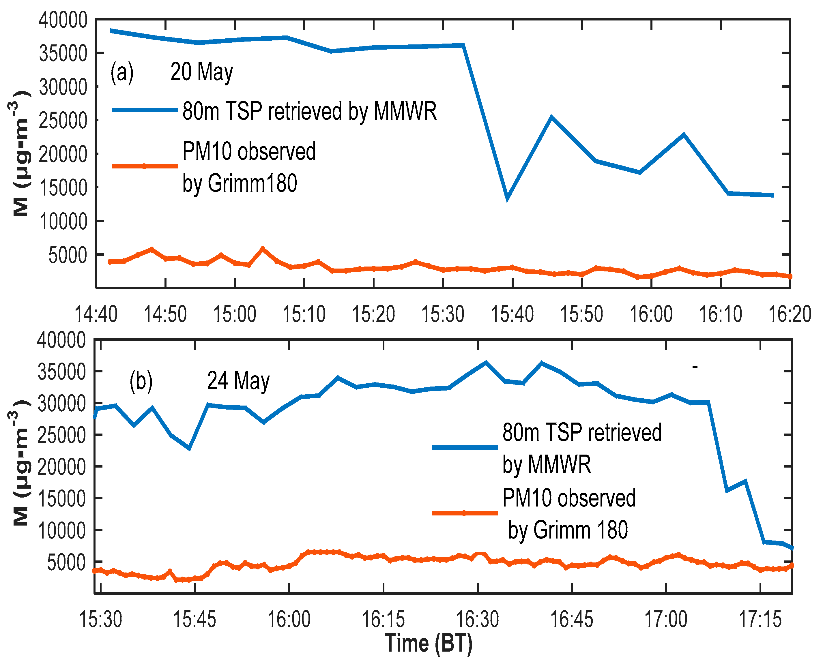
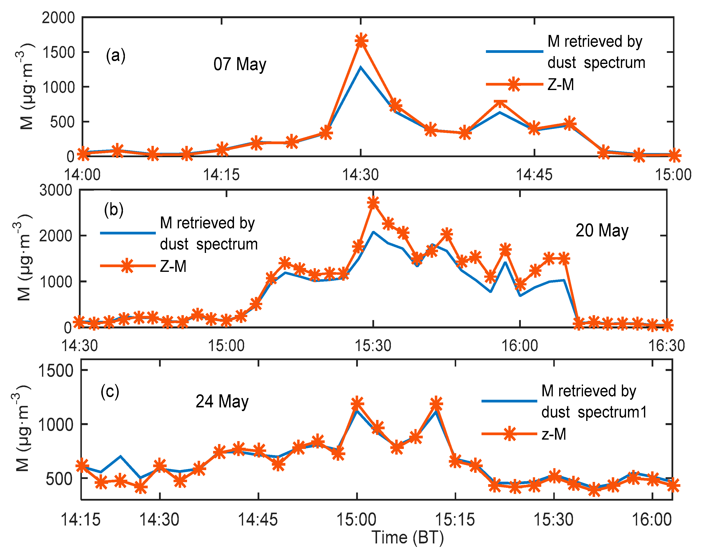
4.5. Dust Mass Concentration

Dust mass concentration is the total mass of the dust particles per unit volume ($1{\mathrm{m}}^3$). Dust mass concentration can be described by $M$ dust spectrum distribution $N\left(D_i\right)$ as follows:

$$M=\frac{1}{6}\pi \rho {\displaystyle \sum }_{i=1}^{N}N\left(D_i\right)D_i^3\Delta D$$

(10)

where $\mathsf{\rho }$ is the dust density ($2.65\times {10}^3\mathrm{kg}/{\mathrm{m}}^3$).

From the dust spectrum distributions retrieved by the Z and the $p\left(D_i\right)$, the temporal and altitudinal distributions of the dust mass concentration for the three dust storms were calculated via Equation (10), and shown as Figure 9. Compared to Figure 7, the temporal and altitudinal variations of the dust mass concentration exhibit a good consistency with the variations of the reflectivity factor. During the floating dust period, the effective height of the dust mass concentration was lower than 300 m; moreover, the values of mass concentration were less than ${10}^{1.5}\mathsf{\mu }\mathrm{g}·{\mathrm{m}}^{-3}$ when the height was 200 m. During the blowing sand period, the effective height of the dust mass concentration was lower than 600 m; furthermore, the values of dust mass concentration were around ${10}^{2.5}\mathsf{\mu }\mathrm{g}·{\mathrm{m}}^{-3}$ at a height of 200 m, and around ${10}^{1.5}\mathsf{\mu }\mathrm{g}·{\mathrm{m}}^{-3}$ at a height of 300 m; whereas, if the height exceeded 400 m, the values of mass concentration were less than ${10}^1\mathsf{\mu }\mathrm{g}·{\mathrm{m}}^{-3}$. During the dust storm period, the effective height of the detected mass concentrations was higher than 1000 m.

The distribution ranges and the average values of the dust mass concentration at different heights during the dust storm period are shown in

Table 5. The distribution features of dust mass concentration at different heights during the dust storm period.

Height (m)	Range of the Mass Concentration $(\mathsf{\mu }\mathbf{g}·{\mathbf{m}}^{-3})$	Average Mass Concentration $(\mathsf{\mu }\mathbf{g}·{\mathbf{m}}^{-3})$	Statistical Cumulative Time (min)
100	1220~42,146	9287	427
200	32~6815	515	413
500	16~3825	70	285
800	10~1825	36	198
1000	8~1280	28	126
1200	2~820	24	86

. It is shown that the average value of dust mass concentration decreases as the height increases. Moreover, when the height rises from 100 to 200 m, the average value of dust mass concentration drops from $9287\mathsf{\mu }\mathrm{g}·{\mathrm{m}}^{-3}$ to $515\mathsf{\mu }\mathrm{g}·{\mathrm{m}}^{-3}$, with a decrease of $8772\mathsf{\mu }\mathrm{g}·{\mathrm{m}}^{-3}$. Furthermore, when the height goes up from 200 to 500 m, the average value of dust mass concentration declines from $515\mathsf{\mu }\mathrm{g}·{\mathrm{m}}^{-3}$ to $70\mathsf{\mu }\mathrm{g}·{\mathrm{m}}^{-3}$, with a decrease of $445\mathsf{\mu }\mathrm{g}·{\mathrm{m}}^{-3}$. Whereas, when the height increases from 800 m to 1200 m, the average dust mass concentration falls from $36\mathsf{\mu }\mathrm{g}·{\mathrm{m}}^{-3}$ to $24\mathsf{\mu }\mathrm{g}·{\mathrm{m}}^{-3}$, with a decrease of $12\mathsf{\mu }\mathrm{g}·{\mathrm{m}}^{-3}$. Hence, the decrease in dust mass concentration weakens as the height increases.

4.6. Data Comparison

Grimm180 particle detector was used as the tool to supplement the dust storms’ observation, so as to verify the accuracy of the dust mass concentrations retrieved by the MMWR.

The Grimm 180 detector was installed at an 80 m height on the flux tower, and consecutive observation was carried out between 14:40 and 16:20 on 20 May, and between 15:29 and 17:20 on 24 May. Figure 10 shows both the temporal variation of the dust mass concentrations with the particle diameters of less than $10 \mathsf{\mu }\mathrm{m}$ (shown as PM10) observed by Grimm 180 and the temporal variation of the dust mass concentration at a height of 80m (shown as TSP) retrieved from the MMWR. During the blowing sand period (16:08–16:20 on 20 May and 17:10–17:20 on 24 May), the real-time values of PM10 were between $1500\mathsf{\mu }\mathrm{g}·{\mathrm{m}}^{-3}\mathrm{and}4000\mathsf{\mu }\mathrm{g}·{\mathrm{m}}^{-3}$ and the real-time values of TSP were mainly between $5500\mathsf{\mu }\mathrm{g}·{\mathrm{m}}^{-3}\mathrm{and}\mathrm{10,000}\mathsf{\mu }\mathrm{g}·{\mathrm{m}}^{-3}$; moreover, the values of $\frac{\mathrm{PM}10}{\mathrm{TSP}}$ (the proportion of the PM10 observed by Grimm180 to the TSP retrieved by MMWR) were generally larger than 30% in the blowing sand, which is consistent with the result of Liu et al. [41]. During the dust storm period (14:40–16:08 on 20 May and 15:30–17:10 on 24 May), the real-time values of PM10 were between $2000\mathsf{\mu }\mathrm{g}·{\mathrm{m}}^{-3}$ and $5500\mathsf{\mu }\mathrm{g}·{\mathrm{m}}^{-3}$, and the values of TSP were mainly between $\mathrm{25,000}\mathsf{\mu }\mathrm{g}·{\mathrm{m}}^{-3}$ and $\mathrm{40,000}\mathsf{\mu }\mathrm{g}·{\mathrm{m}}^{-3}$. Furthermore, the values of $\frac{\mathrm{PM}10}{\mathrm{TSP}}$ were mainly between 5% and 13% in dust storms, which are consistent with the proportion distributions observed by the LPSA (Figure 3), also consistent with the $\frac{\mathrm{PM}10}{\mathrm{TSP}}$ values of, generally, between 5% and 10% for ten dust storms in the Taklimakan Desert (Huo et al. [42]). Hence, it is proven that the values of the dust mass concentration retrieved from MMWR are basically accurate at low altitude.

When the height exceeds 500 m , due to the lack of other dust mass concentration detection data, the values of the dust mass concentration retrieved by MMWR are not verified directly. Using aircraft measurements, Niu et al. [43] and You et al. [44] studied the dust storms in the Tengger Desert and found that the dust mass concentration ranged$\mathrm{between}10\mathsf{\mu }\mathrm{g}·{\mathrm{m}}^{-3}\mathrm{and}400\mathsf{\mu }\mathrm{g}·{\mathrm{m}}^{-3}$ when the height was from 1000 m to 2000 m . The dust mass concentration range retrieved by MMWR in this paper is basically consistent with their results. Hence, the values of dust mass concentration retrieved by MMWR are basically credible.

4.7. Z–MRelationship

Since both the reflectivity factor Z and the dust mass concentration M can be calculated by the dust spectrum distribution, the temporal and altitudinal variation trend of the reflectivity factor (Figure 7) is consistent with that of the dust mass concentration (Figure 9). The relationship between the reflectivity factor Z and the dust mass concentration M can be defined as:

$$Z=A{M}^b$$

(11)

where both A and b are constants. Logarithms taken on both sides of Equation (11) results in:

$$\lg Z=\lg A+b\lg M$$

(12)

With the reflectivity factors Z of the three dust storm processes detected by MMWR and the values of dust mass concentration M ($\mathrm{g}·{\mathrm{m}}^{-3}$ as the unit) retrieved from the dust spectrum distribution, the parameters $\lg A$ and b of Equation (12) can be obtained by the least square method. Then, A is acquired by taking $\lg A$’s exponent. Then, Equation (11) is as follows:

$$Z=651.6M^{0.796}$$

(13)

By utilizing the 200 m height data of the three dust storms, the temporal variations of the dust mass concentration are calculated with the dust spectrum distribution (by Equation (10)) and the reflectivity factor (by Equation (13)), and it is shown in Figure 11. The variation trends of the dust mass concentration calculated by two different methods are consistent with each other, with little difference in the values. Therefore, Equation (13) which stands for the Z–M relationship, is of certain creditability.

5. Discussions

(1) Since the diameter of dust particles is obviously smaller than that of precipitation, and the complex refractive index of dust particles is smaller than that of precipitation, MMWR with millimeter wavelength is used to detect dust particles more effectively.

(2) Compared with satellite remote sensing and Micro Pulse Lidar, the MMWR is of higher vertical resolution (10 m), as well as temporal resolution (a set of data is generated per 1 min), which enables observations of the reflectivity factors of dust storms in real-time. Based on the retrieved method in this paper, the dust spectrum distributions and dust mass concentrations can be obtained in real-time. Therefore, the MMWR can be regarded as the new instrument for the quantitative detection of dust storms in real-time.

(3) During the dust storms in Taklimakan desert, the range of ground wind speeds is generally from 9 m/s to 11 m/s and the variations of the dust spectrum distributions are very small (Huo et al. [42]; Wang et al. [20]). Hence, both the retrieved method and the conclusions of the paper have certain universal significance for the studies of dust storms in Taklimakan desert.

(4) The Z–M relationship summarized in this paper effectively simplifies the retrieved method of M from Z. The real-time quantitative detection of dust storms, carried out by MMWR, becomes faster.

(5) At present, due to the insufficient upper air sounding data, the accuracy of the retrieved dust mass concentration cannot be verified effectively when the height exceeds 500 m. However, in the future, we will use the air sounding monitors to detect the dust spectrum distributions in the upper height for improving the accuracy of the real-time quantitative monitoring of dust storms by the MMWR.

6. Conclusions

The reflectivity factor, the dust spectrum distribution and the dust mass concentration were retrieved from the power spectrum data of the three dust storm processes detected by Ka-band MMWR at Tazhong station in Taklimakan Desert. The conclusions are as follows:

(1) During the dust storm process, the range of the reflectivity factors was$-25\mathrm{dBZ}\mathrm{to}-25\mathrm{dBZ}$. The effective detection height was normally lower than 300 m during the floating dust period, whereas, it was less than 600 m during the blowing sand period, and the detection height was within 2000 m during the dust storm period.

(2) During the floating dust period, the effective height of the dust spectrum distribution was lower than 300 m, and the range of the particles’ diameters was quite small. At a height of 200 m, the dust mass concentration was less than 31.62 $\mathsf{\mu }\mathrm{g}·{\mathrm{m}}^{-3}$.

(3) During the blowing sand period, the effective height of the dust spectrum distribution was lower than 600 m. The range of the particle’s diameter was $0–300\mathsf{\mu }\mathrm{m}$ at a height of 200 m, with a maximum particle number reaching $3162.3$, and the dust mass concentration was less than 316.2 $\mathsf{\mu }\mathrm{g}·{\mathrm{m}}^{-3}$.

(4) During the dust storm period, the effective height of the dust spectrum distribution exceeded 1000 m. At heights less than 500 m, the range of the particles’ diameters was $0–300\mathsf{\mu }\mathrm{m}$, with a maximum number of particles of more than $3162.3$. Similarly, the range of the particles’ diameters was $0–100\mathsf{\mu }\mathrm{m}$ at a height of 1000 m, with a maximum particle number of 10.

(5) During the dust storm period, the range of the dust mass concentration was $1220–42146\mathsf{\mu }\mathrm{g}·{\mathrm{m}}^{-3}$ at a height of 100 m, with the average mass concentration of $9287\mathsf{\mu }\mathrm{g}·{\mathrm{m}}^{-3}$. Meanwhile, the range of the dust masses’ concentrations was $1-1120\mathsf{\mu }\mathrm{g}·{\mathrm{m}}^{-3}$ at a height of 1200 m, with the average mass concentration of$24\mathsf{\mu }\mathrm{g}·{\mathrm{m}}^{-3}$.

(6) The relationship between the reflectivity factor Z and the dust mass concentration M was described as $Z=651.6M^{0.796}$.

References

1. Lau, K.M.; Kim, K.M. Asian summer monsoon anomalies induced by aerosol direct forcing: The role of the Tibetan Plateau. Clim. Dyn. 2006, 26, 855–864. [Google Scholar] [CrossRef]
2. Wang, M.; Wei, W.; Ruan, Z.; He, Q.; Ge, R. Application of wind-profiling radar data to the analysis of dust weather in the Taklimakan Desert. Environ. Monit. Assess. 2013, 185, 4819–4834. [Google Scholar] [CrossRef] [PubMed]
3. Baddock, M.C.; Strong, C.L.; Murray, P.S.; McTainsh, G.H. Aeolian dust as a transport hazard. Atmos. Environ. 2013, 71, 7–14. [Google Scholar] [CrossRef] [Green Version]
4. Sprigg, W.A.; Nickovic, S.; Galgiani, J.N.; Pejanovic, G.; Petkovic, S.; Vujadinovic, M.; Vukovic, A.; Dacic, M.; DiBiase, S.; Prasad, A.; et al. Regional dust storm modeling for health services: The case of valley fever. Aeolian Res. 2014, 14, 53–73. [Google Scholar] [CrossRef] [Green Version]
5. Yan, Y.; Sun, Y.Z.; Ma, L.; Long, X. A multidisciplinary approach to trace Asian dust storms from source to sink. Atmos. Environ. 2015, 105, 43–52. [Google Scholar] [CrossRef]
6. Ramanathan, V.; Crutzen, P.J.; Kiehl, J.T.; Rosenfeld, D. Aerosols, climate, and the hydrological cycle. Science 2001, 294, 2119–2124. [Google Scholar] [CrossRef] [PubMed]
7. Uno, I.; Eguchi, K.; Yumimoto, K.; Takemura, T.; Shimizu, A.; Uematsu, M.; Liu, Z.; Wang, Z.; Hara, Y.; Sugimoto, N. Asian dust transported one full circuit around the globe. Nat. Geosci. 2009, 2, 557–560. [Google Scholar] [CrossRef]
8. Mallet, M.; Tulet, P.; Serca, D.; Solmon, F.; Dubovik, O.; Pelon, J.; Pont, V.; Thouron, O. Impact of dust aerosols on the radiative budget, surface heat fluxes, heating rate profiles and convective activity over West Africa during March 2006. Atmos. Chem. Phys. 2009, 9, 7143–7160. [Google Scholar] [CrossRef] [Green Version]
9. Prospero, J.M.; Lamb, P.J. African droughts and dust transport to the Caribbean: Climate change implications. Science 2003, 302, 1024–1027. [Google Scholar] [CrossRef]
10. Kaufman, Y.J.; Koren, I.; Remer, L.A.; Tanre, D.; Ginoux, P.; Fan, S. Dust transport and deposition observed from the Terra-Moderate resolution Imaging Spectroradiometer (MODIS) spacecraft over the Atlantic Ocean. J. Geophs. Res. 2005, 110, D10S12. [Google Scholar] [CrossRef]
11. Reid, J.S.; Koppmann, R.; Eck, T.K.; Eleuterio, D.P. A review of biomass burning emissions part II: Intensive physical properties of biomass burning particles. Atmos. Chem. Phys. 2005, 5, 799–825. [Google Scholar] [CrossRef]
12. Ganor, E.; Stupp, A.; Alpert, P. A method to determine the effect of mineral dust aerosols on air quality. Atmos. Environ. 2009, 43, 5463–5468. [Google Scholar] [CrossRef]
13. Mamouri, R.E.; Ansmann, A. Fine and coarse dust separation with polarization lidar. Atmos. Meas. Tech. Discuss. 2014, 7, 5173–5221. [Google Scholar] [CrossRef]
14. Mamouri, R.E.; Ansmann, A.; Nisantzi, A.; Solomos, S.; Kallos, G.G.; Hadjimitsis, D. Extreme dust storm over the eastern Mediterranean in September 2015: Satellite, lidar, and surface observations in the Cyprus region. Atmos. Chem. Phys. 2016, 16, 13711–13724. [Google Scholar] [CrossRef]
15. Lei, H.; Wang, J.X.L. Observed characteristics of dust storm events over the western United States using meteorological, satellite, and quality measurements. Atmos. Chem. Phys. 2014, 14, 7847–7857. [Google Scholar] [CrossRef]
16. Kai, K.; Nagata, Y.; Tsunematsu, N.; Matsumura, T.; Kim, H.S.; Matsumoto, T.; Hu, S.; Zhou, H.; Abo, M.; Nagai, T. The structure of the dust layer over the Taklimakan Desert during the dust storm in April 2002 as observed using a depolarization lidar. J. Meteorol. Soc. Jpn. 2008, 86, 1–16. [Google Scholar] [CrossRef]
17. Naeger, A.R.; Christopher, S.A.; Johnson, B.T. Multiplatform analysis of the radiative effects and heating rates for an intense dust storm on 21 June 2007. J. Geophys. Res. Atmos. 2013, 118, 9316–9329. [Google Scholar] [CrossRef]
18. Scheuvens, D.; Schuetz, L.; Kandler, K.; Ebert, M.; Weinbruch, S. Bulk composition of northern African dust and its source sediments—A compilation. Earth Sci. Rev. 2013, 116, 170–194. [Google Scholar] [CrossRef]
19. Mallet, M.; Dulac, F.; Formenti, P.; Nabat, P.; Sciare, J.; Roberts, G.; Pelon, J.; Ancellet, G.; Tanré, D.; Parol, F.; et al. Overview of chemistry-aerosol Mediterranean experiment/aerosol direct radiative forcing on the Mediterranean climate (ChArMEx/ADRIMED) summer 2013 campaign. Atmos. Chem. Phys. 2016, 16, 455–504. [Google Scholar] [CrossRef]
20. Wang, M.Z.; Ming, H.; Huo, W.; Xu, H.X.; Li, J.G.; Li, X.C. Detecting sand-dust storms using a wind-profiling radar. J. Arid Land 2017, 9, 753–762. [Google Scholar] [CrossRef]
21. Takano, T.; Yamaguchi, J.; Abe, H.; Futaba, K.I.; Yokote, S.I.; Kawamura, Y.; Takamura, T.; Kumagai, H.; Ohno, Y.; Nakanishi, Y.; et al. Development and performance of Millimeter-Wave cloud profiling radar at 95 GHZ: Sensitivity and spatial resolution. IEEJ Trans. Fundam. Mater. 2010, 93, 42–49. [Google Scholar] [CrossRef]
22. Wang, Y.; Wang, C.H.; Shi, C.Z.; Xiao, B.H. Integration of cloud top heights retrieved from FY-2 meteorological satellite radiosonde, and ground-based millimeter wavelength cloud radar observations. Atmos. Res. 2018, 214, 284–295. [Google Scholar] [CrossRef]
23. Wang, Z.; Wang, Z.H.; Cao, X.Z.; Tao, F. Comparison of cloud top heights derived from FY-2 meteorological satellites with heights derived from ground-based millimeter wavelength cloud radar. Atmos. Res. 2017, 199, 113–127. [Google Scholar] [CrossRef]
24. Bryan, S.; Clarke, A.; Vanderkluysen, L.; Groppi, C.; Paine, S. Measuring water vapor and Ash in Volcanic Eruptions with a millimeter-wave radar/imager. IEEE Trans. Geosci. Remote Sens. 2017, 55, 3177–3184. [Google Scholar] [CrossRef]
25. Zhao, C.; Liu, L.; Wang, Q.; Qiu, Y.; Wang, Y.; Wu, X. MMCR-based characteristic properties of non-precipitation cloud liquid droplets at Naqu site over Tibetan Plateau in July 2014. Atmos. Res. 2017, 190, 68–76. [Google Scholar] [CrossRef]
26. Ayhan, S.; Pauli, M.; Scherr, S.; Göttel, B.; Bhutani, A.; Thomas, S.; Jaeschke, T.; Panel, J.M.; Vivier, F.; Eymard, L.; et al. Millimeter-wave radar sensor for snow height measurements. IEEE Trans. Geosci. Remote Sens. 2017, 55, 854–861. [Google Scholar] [CrossRef]
27. Chen, H.Y.; Ku, C.C. Calculation of wave attenuation in sand and dust storms by the FDTD and turning bands methods at 10–100 GHz. IEEE Trans. Antennas Propag. 2012, 60, 2951–2960. [Google Scholar] [CrossRef]
28. Dong, Q.F.; Li, Y.L.; Xu, J.D.; Zhang, H.; Wang, M.J. Effect of sand and dust storms on microwave propagation. IEEE Trans. Antennas Propag. 2013, 61, 910–9162. [Google Scholar] [CrossRef]
29. Dong, Q.F.; Li, Y.L.; Xu, J.D.; Zhang, H.; Wang, M.J. Backscattering characteristics of millimeter wave radar in sand and dust storms. J. Electromagn. Wave Appl. 2014, 28, 1075–1084. [Google Scholar] [CrossRef]
30. Juan, W.; Li, X.; Wang, M.; Sun, W. Theoretical analysis of potential applications of microwave radar for sandstorm detection. Theor. Appl. Climatol. 2019, 137, 1–6. [Google Scholar] [CrossRef]
31. Nashashibi, A.Y.; Sarabandi, K.; Al-Zaid, F.A.; Alhumaidi, S. Characterization of radar backscatter response of sand-covered surfaces at Millimeter-Wave frequencies. IEEE Trans. Geosci. Remote Sens. 2012, 50, 2345–2354. [Google Scholar] [CrossRef]
32. Yuan, H.; Zhuang, G.; Li, J.; Wang, Z.; Li, J. Mixing of mineral with pollution aerosols in dust season in Beijing: Revealed by source apportionment study. Atmos. Environ. 2008, 42, 2141–2157. [Google Scholar] [CrossRef]
33. Choobari, O.A.; Zawar-Reza, P.; Sturman, A. The global distribution of mineral dust and its impacts on the climate system: A review. Atmos. Res. 2014, 138, 152–165. [Google Scholar] [CrossRef]
34. Liu, L.X.; Huang, X.; Ding, A.J.; Fu, C.B. Dust- induced radiative feedbacks in north China: A dust storm episode modeling study using WRF-Chem. Atmos. Environ. 2016, 129, 43–54. [Google Scholar] [CrossRef]
35. Chen, S.; Huang, J.P.; Zhao, C.; Qian, Y.; Leung, L.R.; Yang, B. Modeling the transport and radiative forcing of Taklimakan dust over the Tibetan plateau: A case study in the summer of 2006. J. Geophys. Res. Atmos. 2013, 118, 797–812. [Google Scholar] [CrossRef]
36. Rashki, A.; Arjmand, M.; Kakaoutis, D.G. Assessment of dust activity and dust- plume pathways over Jazmurian Basin, southeast Iran. Aeolian Res. 2017, 24, 145–160. [Google Scholar] [CrossRef]
37. Rashki, A.; Kaskaoutis, D.G.; Sepehr, A. Statistical evaluation of the dust events at selected stations in Southwest Asia: From the Caspian Sea to the Arabian Sea. Catena 2018, 165, 590–603. [Google Scholar] [CrossRef]
38. Zhang, P.C.; Du, B.Y.; Dai, T.P. Radar Meteorology; China Meteorological Press: Beijing, China, 2000; pp. 77–87. (In Chinese) [Google Scholar]
39. Dong, Q.S. Physical characteristics of the sand and dust in different deserts of China. Chin. J. Radio Sci. 1997, 12, 15–25. (In Chinese) [Google Scholar]
40. Dong, Z.B.; Man, D.Q.; Luo, W.Y.; Qian, G.Q.; Wang, J.H.; Zhao, M.; Liu, S.Z.; Zhu, G.Q.; Zhu, S.J. Horizontal aeolian sediment flux in the Minqin area, a major source of Chinese dust storms. Geomorphology 2010, 116, 58–66. [Google Scholar] [CrossRef]
41. Liu, X.C.; Zhong, Y.T.; He, Q. Ali MMTM, Observation study on mass concentration of dust aerosols in the Taklimakan Desert hinterland. China Environ. Sci. 2011, 31, 1609–1617. (In Chinese) [Google Scholar]
42. Huo, W.; He, Q.; Yang, F.; Yang, X.; Yang, Q.; Zhang, F.; Mamtimin, A.; Liu, X.; Wang, M.; Zhao, Y.; et al. Observed particle sizes and fluxes of Aeolian sediment in the near surface layer during sand—Dust storms in the Taklamakan Desert. Theor. Appl. Climatol. 2017, 130, 735–746. [Google Scholar] [CrossRef]
43. Niu, S.J.; Sun, Z.B. Aircraft measurements of sand aerosol over Northwest China desert area in late spring. Plateau Meteorol. 2005, 24, 604–610. (In Chinese) [Google Scholar]
44. You, L.G.; Ma, P.M.; Chen, J.H.; Li, K. A case study of the aerosol characteristics in the lower troposphere during a dust storm event. J. Appl. Meteorol. Sci. 1991, 2, 13–21. (In Chinese) [Google Scholar]
Figure 1. (a) Ka-band millimeter continuous wave radar; (b) the geographic position of Tazhong.
Atmosphere 10 00511 g001
Figure 2. The retrieval process of the dust spectrum distribution. (a) The power spectrum S ( f i ) . (b) The particle probability distribution p ( D i ) . (c) The dust spectrum distribution N ( D i ) .
Atmosphere 10 00511 g002
Figure 3. The particle proportion distributions obtained by the Laser Particle Size Analyzer (LPSA) (a) 7 May (b) 20 May (c) 24 May.
Atmosphere 10 00511 g003
Figure 4. The fitted lognormal distributions of dust particles proportions at the 47 m, 63 m and 80 m heights of the three dust storms (a) 07 May (b) 20 May (c) 24 May.
Atmosphere 10 00511 g004aAtmosphere 10 00511 g004b
Figure 5. The 500 hPa geopotentialheight fields (10 m) (a) at 08:00 on 18 May and (b) at 08:00 on 20 May.
Atmosphere 10 00511 g005
Figure 6. The ground wind speed on (a) 7 May, (b) 20 May and (c) 24 May.
Atmosphere 10 00511 g006
Figure 7. The temporal and altitudinal distribution of the reflectivity factor. (a) 7 May. (b) 20 May. (c) 24 May.
Atmosphere 10 00511 g007
Figure 8. The altitudinal distribution of the dust spectrum distribution. (a) The floating dust at 10:00, (b) the blowing sand—12:32 and (c) the dust storm at 16:00.
Atmosphere 10 00511 g008
Figure 9. The temporal and altitudinal distributions of dust mass concentrations on (a) 7 May, (b) 20 May and (c) 24 May.
Atmosphere 10 00511 g009
Figure 10. The temporal variation of the 80m height dust mass concentration retrieved from millimeter wave radar (MMWR) data and the temporal variation of the PM10 from Grimm180. (a) 20 May, (b) 24 May.
Atmosphere 10 00511 g010
Figure 11. The temporal distribution of dust mass concentration at a height of 200 m. (a) 14:00–15:00 on 7 May; (b) 14:30–16:30 on 20 May; (c) 14:15–16:00 on 24 May.
Atmosphere 10 00511 g011