1. Introduction
In the past two to three decades, computational modeling has emerged as such an important approach for scientific discovery that numerical simulation is considered by many as a third pillar of science [
1]. Coupled with the increasing application of computational modeling in the sciences is the surging need for analyzing the enormous amount of data it generates. Scientific visualization is an intuitive, yet powerful approach to explore, analyze, and present large and complex data and is thus considered to be critical to the understanding of simulation outputs [
2]. Elementary visualization methods such as line plotting, contouring, color mapping, and scatter plots are fundamental to scientific workflows, and examples of such are found in nearly every scientific journal article. Yet, these basic techniques are limited in their ability to convey information and provide insight in the face of increasing data size and complexity, particularly for data with three spatial dimensions (3D).
Largely because of the challenges posed by 3D data, a vibrant visualization research community exists and is continuously evaluating and innovating new methods for exploring large and complex data. The most successful of these “advanced” techniques are often deployed in software packages either as stand-alone tools or as part of a menu of selectable visualization algorithms within an application. Two representatives of such software packages are VisIt [
3] and ParaView [
4]. Both have Graphical User Interfaces (GUIs), making them well-suited for interactive exploratory work. However, though general purpose and highly capable, these tools face unique challenges posed by Earth System Sciences (ESS), such as: (1) lack of support for geo-referenced information, (2) inability to handle large data on commodity hardware effectively, and (3) lack of support for the unique visualization requirements found in ESS.
On the other hand, software packages designed specifically for visualizing ESS data exist as well. However, most of these are implemented as a collection or library of functions exposed to the user via interpretive languages or through a Command Line Interface (CLI). In other words, they have limited interactivity.
To fill the gap between highly-interactive, general purpose visualization packages and domain-focused, but batch-oriented ones, the National Center for Atmospheric Research (NCAR) developed and first released the VAPOR package in 2007. VAPOR is designed for researchers in the ESS field from modelers to analysts. It combines many of the specialized functionalities required by ESS data visualization with the interactivity and ease of use enabled by a GUI. Moreover, through the use of a clever data model, VAPOR users are able to employ ubiquitous commodity computing to operate on data whose size would otherwise overwhelm such meager computing resources.
Over a decade after its first release, receiving feedback from thousands of users worldwide and learning valuable lessons along the way, NCAR embarked on a new effort to produce the third major release of the VAPOR package. The resulting product, VAPOR Version 3, addresses the shortcomings of the previous releases with three major improvements:
A more flexible data model that supports operating directly on the somewhat specialized computational grids widely used in ESS;
A cleaner software architecture that facilitates the extensibility of new functionalities; and
A more organized user interface that is easier and more intuitive to use.
This paper reflects the state of VAPOR Version 3, and references to the past VAPOR releases can be found in previous publications [
5,
6]. The rest of this paper is organized as follows: After covering related work in
Section 2,
Section 3 provides an architectural overview of VAPOR.
Section 4 and
Section 5 highlight a few unique capabilities of VAPOR that are beneficial to ESS researchers.
Section 6 first describes a use case where VAPOR is used to facilitate analyzing a large-scale tornado simulation, and then highlights VAPOR’s specialties in handling ESS data that are lacking in VisIt and ParaView. After discussing our design choices and future work in
Section 7, we conclude this paper in
Section 8.
2. Related Work
We survey software products related to VAPOR in this section.
Section 2.1 surveys visualization tools for general purpose scientific data analysis, while
Section 2.2 surveys visualization and analysis tools designed specifically for ESS data.
2.1. General Purpose Scientific Visualization Software
Early scientific visualization software programs were mostly developed for specific systems and application environments, limiting both their portability and generality [
7,
8,
9]. More general purpose software programs started to emerge in the 1990s, with the Visualization Toolkit (VTK) [
10] being a representative example. VTK implements a collection of commonly-used visualization algorithms in standard C++, and its object-oriented nature greatly facilitates building entire end-user visualization systems. GUI-based, general purpose visualization software started to emerge in the late 1990s and early 2000s, with VisIt [
3] and ParaView [
4] being some of the longest-lived examples. Both VisIt and ParaView are built on top of VTK. The GUI-based nature of these tools enables quick and easy parameter manipulation needed for interactive data exploration. Moreover, the GUI alleviates the need for programming experience, making visualization accessible to the widest scientific community. A key feature of both VisIt and ParaView is that they support distributed-memory parallelism and are thus capable of operating across multiple compute nodes to process very large datasets.
A recent trend in scientific visualization software development, which is ironically reminiscent of the past, is the emergence of hardware vendor-specific toolkits, such as OSPRay [
11] from Intel and IndeX [
12] from Nvidia. These toolkits are heavily optimized for each vendors’ particular hardware and are claimed to deliver some of the best performance in terms of speed ever reported. These toolkits offer only a small subset of the capability of VTK, providing only highly-optimized and specialized algorithms aimed primarily at volumetric data. Like VTK, they are not intended for use by scientific end-users, but for software developers to use them as building blocks to produce highly-performant tools.
2.2. Earth System Data Analysis Tools
A large variety of open source software packages that specifically target the atmospheric and related sciences are in wide-spread use today. These tools can be loosely categorized into two groups based on their user interfaces: batch tools or scripting languages invoked from the command line and interactive tools with Graphical User Interfaces (GUIs). The former are more widely used in the Earth sciences, particularly in settings where the data are either two-dimensional in space or where the user already has a good sense of how to configure the various visualization parameters (e.g., color maps, contour line values, and region-of-interest) that will determine the resulting images. An example of such a domain where batch tools are predominantly employed is operational weather forecasting. Domains where the data are three-dimensional or the visualization settings are not known in advance (e.g., meteorological research environments) are often better served by more interactive tools whose operation is controlled via a GUI.
One of the most widely-used batch tools is the venerable NCAR Command Language (NCL), which provides a domain-specific scripting language and boasts hundreds of highly-specialized analysis and visualization functions for climate, weather, and ocean data [
13]. Increasingly, batch tools are being developed and made available within the Python ecosystem. A short list of examples include: CDAT [
14], MetPy [
15], and Iris [
16]. While these tools share a common control language, ease of interoperability is far from assured. The recent Pangeo effort [
17] is an attempt to identify and encourage the development of scalable Python tools for the Earth sciences that play well together by leveraging some common building blocks, notably Xarray [
18] and Dask [
19].
Perhaps due in part to their complexity and corresponding increased development cost and in part to lack of user demand, fewer GUI-based tools targeting the atmospheric sciences exist. Vis5D [
20] was a pioneer in interactively visualizing 5D grid data (three spatial dimensions, one temporal, and one variable) such as those from numerical weather models. It supported a number of what were considered advanced 3D visualization techniques at the time, but unfortunately ceased development in 2001. Met.3D [
21], developed by the University of Hamburg, supports data encoded as CF-compliant NetCDF files or ECMWF GRIB files and provides general purpose 3D visualization methods. Met.3D’s niche, however, is its support for analyzing ensemble data using some of the most recently-reported ensemble data analysis methods. McIDAS-V [
22] is another interactive, 3D visualization tool for the Earth sciences. In addition to its ability to operate on gridded data, McIDAS’s real strength is support for geo-referenced data from observational sources, particularly satellite data. Similar to McIDAS, and even sharing the same underlying software framework, is the Interactive Data Viewer (IDV) [
23], developed by Unidata. Like McIDAS, IDV supports both gridded and observational Earth sciences data and is capable of simultaneously combining the two.
An extensive survey of current and past batch and interactive tools can be found in the recent work by [
24].
3. Overview of VAPOR
3.1. Capabilities for Earth System Science
Though possessing many of the same features commonly found in more general purpose interactive visualization packages, such as VisIt and ParaView, VAPOR’s strength as a tool for ESS analysis is its features that are tailored specifically towards ESS needs. We list some of these capabilities in brief here and describe a subset in more detail throughout the rest of this paper.
Geo-referenced data and image files: VAPOR understands geo-referenced data and is able to combine geo-referenced data from multiple sources, visualizing them in a single scene with correct registration. Moreover, geo-referenced coordinates may undergo mapping projections using a number of supported map projection types.
Vertical coordinate systems: In addition to geo-referenced horizontal coordinates, VAPOR supports many of the vertical coordinate systems defined by the CF conventions (e.g., sigma, s-coordinates, and hybrid sigma).
File formats: VAPOR knows how to read many of the file formats and model outputs commonly used in ESS. Most notably, VAPOR understands WRF-ARW, MPAS, and CF-compliant NetCDF files.
Grid types: VAPOR supports computational meshes typical of ESS, such as layered curvilinear grids, layered unstructured grids, and Arakawa grids. Computationally-intensive visualization algorithms (e.g., direct volume rendering) are also optimized for these grid types.
Missing data: VAPOR understands missing data values that are commonly seen in ESS. For example, in ocean models employing lat-lon grids, missing value flags are often used where the computational mesh intersects land masses.
3.2. Software Architecture
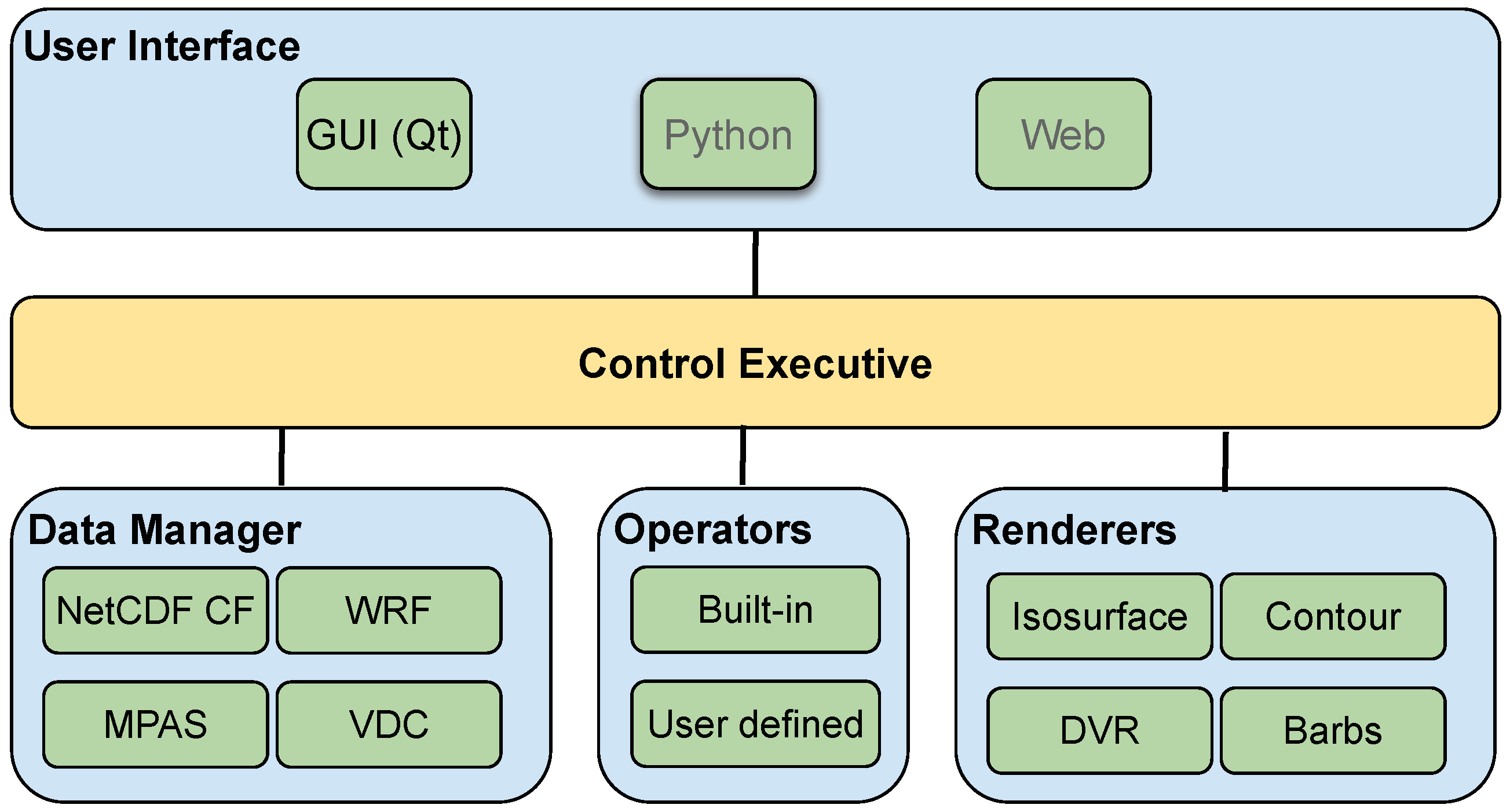
VAPOR is a desktop application implemented mostly in C++. The main software components are depicted in
Figure 1. Currently, the user interacts with VAPOR though a GUI, which is implemented using Qt: a platform-portable GUI toolkit that enables a common user interface across three major operating systems (macOS, Linux, and Windows). A scripting interface (most likely Python) is planned for the future, as is a web interface. The user interface, whether a GUI or a script, communicates user requests to a
Control Executive, which interacts with the remaining three major components of VAPOR:
Data Manager: the component that holds the underlying data, hides file formats and computational grid details, and provides unified data access to the rest of the application;
Operators: a collection of functions that perform calculations on the data prior to rendering; and
Renderers: a collection of C++ class objects that implement various 2D and 3D visualization algorithms (e.g., contour lines, isosurfaces, volume rendering, and wind barb plots).
3.3. Data Manager
The Data Manager is responsible for reading gridded data (referred to as “variables”) from a file or files (or possibly a data service) and making these variables available, along with any metadata, to the rest of the application. The Data Manager presents an abstract representation of gridded data that hides the underlying storage details and to a large degree hides details about the computational grid itself. Clients of the Data Manager, in general, need not be concerned about the grid’s topology (structured or unstructured), geometry (e.g., rectilinear and curvilinear), or VAPOR-specific properties (multi-resolution and lossy compression). Other components in the application can query the Data Manager for a list of variable names available in the data collection, the names of the coordinate variables associated with each data variable, the number of time steps present, and so on. In addition to metadata, the Data Manager also satisfies requests to access a named variable at a specific time step and region in space. Variables returned by the Data Manager are not simple arrays of floating point values, but C++ class objects that support a wide variety of operations to facilitate visualization, such as returning the interpolated value of a point in space or returning the user coordinates for a node in the mesh.
Since analysis and visualization are often I/O-bound operations, the Data Manager takes steps to reduce I/O costs. Principle among these is to store variables as they are accessed in a memory-resident Least Recently Used (LRU) cache. Subsequent accesses to a variable that is currently in the cache will avoid disk reads. The size of the cache is controlled by the user and may be as large as that the host platform will allow.
Currently, the Data Manager is capable of reading a number of commonly-used ESS file formats such as CF-compliant NetCDF [
25], WRF-ARW [
26], MPAS-A [
27], and MPAS-O [
28]. Additionally, the Data Manager can read VAPOR Data Collection (VDC) with multi-resolution and lossy compression properties. Details of the VDC are discussed in
Section 4.
3.4. Operators
VAPOR supports both built-in and user-defined data operators. The former is primarily concerned with transforming mesh coordinate variables. For example, applying projections to map horizontal geographical coordinate systems into “meters-on-the-ground” projected coordinates or transforming one of the many vertical coordinate systems used in ESS to units of height above (or below) the Earth’s surface. In addition to built-in operators, VAPOR offers an embedded Python interpreter to define custom operators. Existing variables may be passed to the interpreter, operated on by user-defined Python scripts, and returned to the application as a derived quantity. For example, the user might define a Python script to derive vorticity from the components of velocity.
3.5. Renderers
VAPOR implements a suite of 2D and 3D visualization algorithms called “renderers,” some of which are very basic (e.g., line contouring), while others are quite advanced (e.g., direct volume rendering). In many cases, creating visualization algorithms are comprised of two steps: mapping numerical data into a collection of some form of displayable graphical primitives, and the rendering of those primitives to an image. The latter operation, rendering, is performed using the platform-portable OpenGL 3D rendering library, which is highly optimized for high-performance rendering on Graphics Processing Units (GPUs). This means that VAPOR achieves the best performance when GPUs are present in the system, though it is also capable of operating without GPUs via software implementations of OpenGL that execute on the CPU.
Section 5 provides more information on the renderers available in VAPOR, and
Section 7.1 further discusses the design choice of using OpenGL in the application.
3.6. Extensibility
VAPOR is an open development package; thus, any aspect of the code might be enhanced by the user community. However, the architecture of VAPOR is designed to facilitate three specific forms of extension: (1) addition of new user interfaces; (2) addition of new data readers; and (3) addition (or enhancement) of new (existing) visualization renderers. This goal is achieved via reusable GUI elements and well-defined procedures for such operations.
The addition of new GUI elements is facilitated with a collection of composite Qt widgets, which implement controls for the most common functionalities of VAPOR. Examples of these controls include variable selectors, transfer function editors, and geometry boundary editors. These composite widgets are composed of primitive Qt widgets to provide desired controls and also use consistent layout and size policies to provide a uniform look. The author of a new user interface is then able to reuse these composite widgets in a plug and play fashion.
For the addition of new data readers, let us consider a scenario where a new data importer is needed to support a new data format. This is relatively easy with VAPOR’s C++ object-oriented implementation and involves only deriving a single data reader class object from an existing interface class. An interface class specifies the functions a derived class will need to implement. For example, a data reader-derived class must implement a C++ method (function) that returns a list of all of the variable names contained in a dataset. Similarly, the derived data reader class will need to implement a function that will read a hyper-slice of data for a specified variable and return the data as an array of floating point values. As a reference, the source file for reading WRF-ARW data is approximately 1000 lines of code.
For the addition of new visualization renderers, let us consider a scenario where a new renderer is required to support a novel rendering technique. This is a more complex extension, since it involves both the Renderer and GUI components. The basic steps involve: (1) implementing the actual rendering algorithm, which will operate on data returned from the Data Manager, and producing a rendering by making appropriate calls to OpenGL; and (2) creating the corresponding user interface to expose and control the various rendering parameters required by the new renderer. As with the previous case, in both of these steps, the minimally-required programming interface is already defined via C++ interface classes, and the implementer need only author the new classes using the interface classes as a recipe. The renderer author will also need to provide a new user interface to support control parameters that are generic (e.g., variable selection), as well as specific to the new renderer. This step again is simplified by making use of the reusable composite Qt widgets.
4. VAPOR Data Collection
Maintaining interactive performance while visualizing and analyzing high-resolution simulation data is a challenging task. Storage capacity, bandwidth, and computational requirements may all limit the rate at which data can be processed and displayed on the screen. One approach for addressing this challenge is the use of progressive data access: reduced-size approximations of the data are used for quick-look, exploratory work, and then subsequently refined with more accurate data representations to produce a final rendering or analysis.
A straightforward way to support progressive data access that is widely employed by digital mapping technologies such as Google MapsTM is multi-resolution: coarsened imagery (data) is transmitted and displayed when the viewpoint is far away and continuously refined as the user zooms in on a region of interest.
Most commonly, multi-resolution representations are simply a hierarchy of approximations created by successively coarsening the original gridded data, reducing the number of grid points along each dimension by a factor of two with each pass. There are a number of ways to generate multi-resolution data representations. Sampling the original data points and storing them separately as lower resolution versions is perhaps the simplest one. However, this strategy incurs storage overhead from maintaining separate versions of the data. Space filling curves (e.g., Z-curves [
29] and Hilbert curves [
30]) offer a way to sample and organize the data without incurring storage overhead. While they do not increase storage, the quality of the coarsened approximations resulting from sampling can be quite poor.
A method for achieving higher quality approximations without additional storage is through the use of discrete wavelet transforms [
31,
32]. Much like discrete Fourier transforms that map data between physical and frequency space, wavelet transforms map data from physical space into a collection of output coefficients (i.e., “
wavelet coefficients”) that live in the wavelet domain. The wavelet transforms are reversible, and exact reconstruction of the original data is possible up to floating point round off error. With a suitable choice of wavelet, the number of wavelet coefficients will equal the number of grid points, thus not changing storage requirements.
4.1. Wavelet Transforms in VAPOR Data Collection
Most of interest to our discussion is the multi-resolution properties of wavelets, which permit reconstruction of approximations of the original data at roughly power-of-two grid resolutions, creating a hierarchy of data. Moreover, the reconstructed approximations are weighted averages of neighboring samples, yielding higher quality approximations than sampling.
Many wavelets possess another property that is relevant to progressive data access,
information compaction, meaning that most of the information contained in a signal (or gridded dataset) will be contained in a small subset of the wavelet coefficients. A second form of progressive data access can be realized by ordering the coefficients based on their information content and using only the most important ones for reconstruction. This practice of culling wavelet coefficients is often referred to as
lossy compression, which has already been shown to reduce overall I/O time on large parallel systems [
33], and similar techniques are also widely used in consumer products from JPEG images to streaming audios and videos.
Thus, two forms of data reduction are possible with wavelets, each, however, with different characteristics. On the one hand, multi-resolution yields a coarsened grid, reducing the computation and memory cost of operations performed on the reconstructed data. On the other hand, lossy compression has no bearing on grid resolution and subsequent costs of operating on the reconstructed data. In other words, lossy compression offers no benefit to compute or memory bound tasks.
VAPOR uses wavelet transforms in its VAPOR Data Collection (VDC) with support for both forms of progressive data access: multi-resolution and lossy compression. As a result, the VDC enables interactive explorations of very large data with progressive data access. Essentially, the user is afforded the ability to make speed/quality tradeoffs. In practice, VAPOR exposes both multi-resolution and lossy compression controls in the GUI, enabling advanced users to fine-tune different combinations of these two parameters based on their knowledge of system bottlenecks. For novices, VAPOR also provides a simpler, unified linear “fidelity” control that incorporates both controls ranging from the lowest fidelity (i.e., lowest resolution and maximum lossy compression) to the highest fidelity (i.e., original resolution and no lossy compression).
We note that VDC is optional for the users: VAPOR can directly import popular data formats in the ESS field (e.g., WRF and CF-Compliant NetCDF) or convert them to VDC format and then import the VDC files. The conversion tools are packaged and distributed with VAPOR.
Finally, the general topic of scientific data reduction is a quite complex and active research area. This survey [
34] provides an overview of this topic.
4.2. VDC Enabled Workflow
The VDC format enables a unique workflow that is suited for data exploration and follows Shneiderman’s information visualization mantra: “Overview first, zoom and filter, then details-on-demand” [
35].
Using this workflow, the users can start exploring a given large dataset at lower fidelity levels. This process can iterate rather rapidly until the user has located areas of interest in space and/or time, selected viewpoints in the case of 3D data, and selected visualization techniques and their parameters such as color maps, isovalues, etc.
The user can then increase the fidelity level to examine more details and keep fine-tuning the visualization parameters. Once satisfied with various visualization parameters, the user might select the highest data fidelity to render final visualizations at the highest quality for purposes such as publishing or verification of results found with lower fidelity data.
4.3. Examining VDC performance
To further explore and quantify the benefits of the VDC data format, we report a few findings from an evaluation of VDC performance using a commodity computing platform and a relatively large dataset. These tests were performed on a Linux desktop with the specifications listed in
Table 1. The test data were one time step of vorticity magnitude from a Taylor–Green turbulence simulation [
36]. This dataset had 32-bit floating point values sampled on a regular grid with a resolution of 1024
3. Vorticity was chosen for our analysis because it is particularly challenging for any data compression due to the presence of many fine-scale structures.
4.3.1. Interactivity Improvement
We first explored the benefits to interactivity. When performing data analysis and visualization, interactivity is usually impacted by two operations: reading data from the disk (I/O) and rendering (computation). With VDC, the former impact is mitigated by both forms of progressive data access, while the latter is solely mitigated by lower resolutions. The I/O impact, however, is difficult to measure in a consistent manner due to complex caching mechanisms baked in to modern operating systems. As a result, here we will only provide measures on the computational impact.
We used frames-per-second (FPS) to measure the interactivity, so higher FPS indicates better interactivity. Two computationally intensive 3D renderers were tested: direct volume rendering and isosurface rendering. For each resolution, we used similar rendering parameters so that the resulting renderings looked approximately the same and then tested the FPS with those parameters.
Table 2 reports the test results, with each frame rate being averaged from twenty test runs. These numbers show that, not surprisingly, lower resolutions effectively improve interactivity.
4.3.2. Rendering Quality Impact
Multi-resolution representations and lossy compression will of course negatively impact rendering quality. Among these two factors, multiple resolutions have a significantly bigger impact for a given amount of data reduction. We illustrate this impact with different renderings and provide a qualitative evaluation; more quantitative analysis can be found in our previous work [
37,
38].
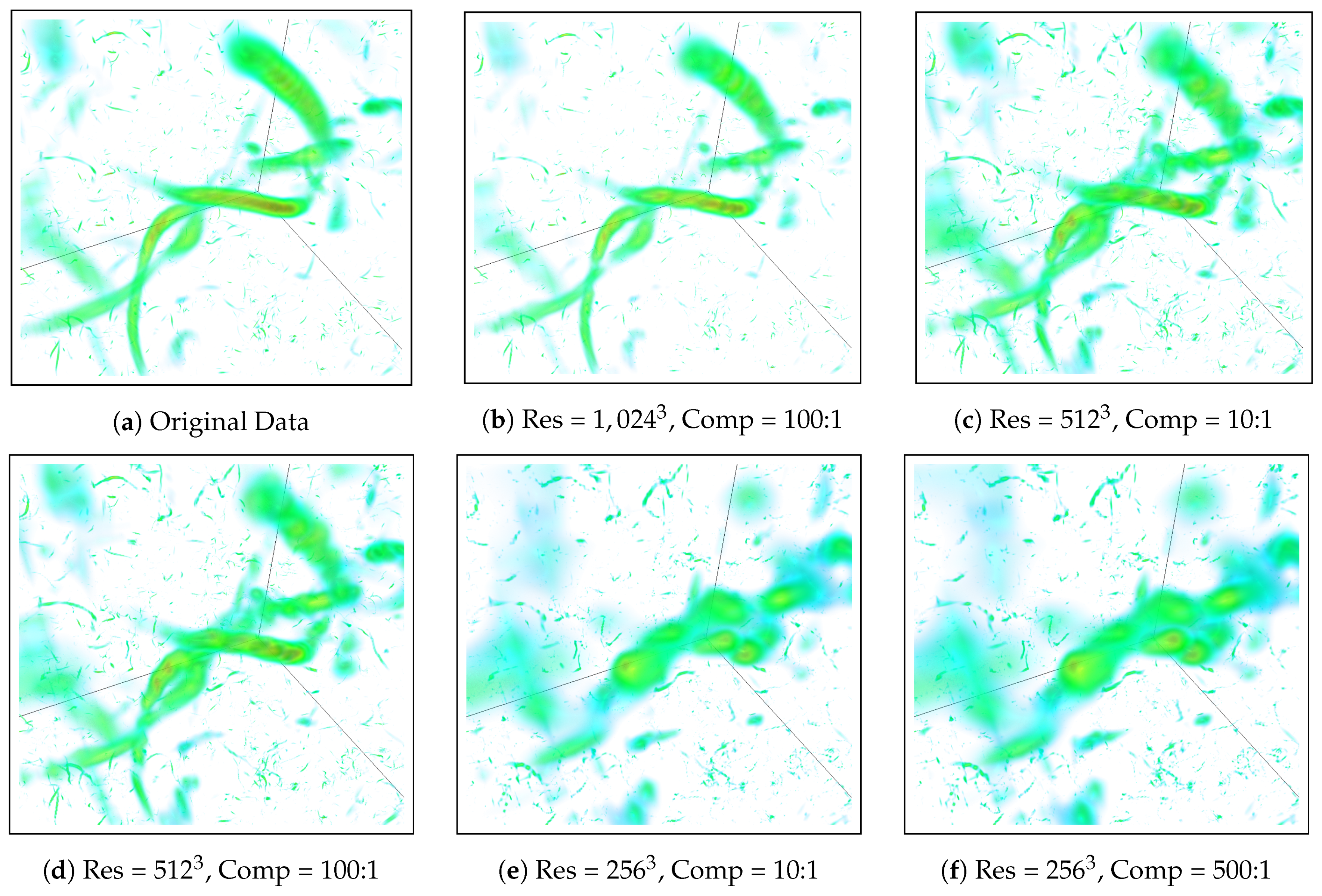
We used volume rendering to visualize the high-vorticity areas, which look like worms or filaments in a turbulent flow.
Figure 2 highlights one such area that contains a few filaments, which appear in green. Given the original data resolution of 1024
3, renderings at 512
3 still can identify and show the basic shapes of filaments, while renderings at 256
3 lose most details of the identified filaments. These renderings also show results from lossy compression and that lossy compression does not degrade renderings nearly as significantly as lower resolutions. Overall, many of the reduced data renderings still contained sufficient information to establish visualization parameters and perhaps obtain a holistic qualitative understanding of the data.
4.3.3. Computational Impact
This subsection reports the computational cost of performing wavelet transforms, both forward and inverse. The forward transform is usually performed only once to convert the original data into VDC format, while the inverse transform is performed whenever VAPOR is retrieving data from the disk. We remind the reader, however, that VAPOR’s Data Manager is able to cache recently-used data to avoid repeated reconstructions. Another difference is that the forward transforms are performed to prepare all resolution levels, incurring a fixed cost, while the inverse transforms are performed for just enough iterations to retrieve a certain resolution level, incurring a varying cost.
Table 3 reports computational costs for preparing a data of 1024
3 resolution to VDC format, and reconstructing it back to gridded data in various resolutions. Note that both operations are asymmetric in that reconstruction takes much less time. Since VDC conversions are implemented in parallel in VAPOR, these numbers can vary drastically from system to system.
4.3.4. Storage Impact
Lossy compression allows VAPOR to use either a
portion or
all of the wavelet coefficients to reconstruct an
approximate or
faithful version of the original data. This capability, however, requires extra storage for coefficient addressing, resulting in the fact that when targeting an
compression ratio by using
of all coefficients, the actual storage size is more than
of the original data size.
Table 4 reports this storage overhead at default compression ratios when converted data are stored in VDC format.
5. Visualization Renderers
VAPOR provides visualization renderers for both two-dimensional and three-dimensional data. The two-dimensional renderers in VAPOR are similar to the corresponding renderers found in batch-processing visualization packages (e.g., NCL); they include:
Contour Render: calculates and renders a series of topographic-style contours lines;
Barb Renderer: encodes field values as arrows in different directions and lengths; and
2D Pseudocolor Renderer: maps data values from a two-dimensional variable to different colors.
The rest of this section first provides an overview of common visualization controls that enable users to manipulate renderer parameters in the VAPOR GUI and then describes three-dimensional renderers and the Image Renderer that is unique to VAPOR. The three-dimensional renderers to be discussed are:
5.1. Common Visualization Controls
VAPOR’s visualization renderers use different algorithms for image rendering, but they share a set of common controls in the VAPOR application. These common controls are presented using reusable composite Qt widgets as discussed in
Section 3.6, and their functionalities include selections for variables, VDC data fidelity, geometry boundaries, affine transformations, annotations, transfer functions, etc. Among the common GUI components, the transfer function editor serves a critical role in data exploration and the creation of informative visualizations, so we describe it in detail.
The transfer function editor allows users to define a pair of functions that map data values of a variable to color and opacity, respectively. To adjust color mapping, the user first chooses a color palette (either from pre-installed ones or custom designs) and then designates a range of data values to be covered by this color palette. To adjust opacity mapping, the user drag-and-drops control points on a sequence of line segments, so the shape of these line segments represents the variation of opacity across the designated value range. The result is that each data value is associated with a unique combination of color and opacity. Data values outside of the designated value range will receive colors and opacity on the range boundaries. After achieving a satisfactory rendering, the user can save the transfer function in a file for future use.
The VAPOR transfer function editor further augments user selections by embedding a data histogram within the editor, so the users are always informed of the relative data frequency of each value and can assign color and opacity values accordingly.
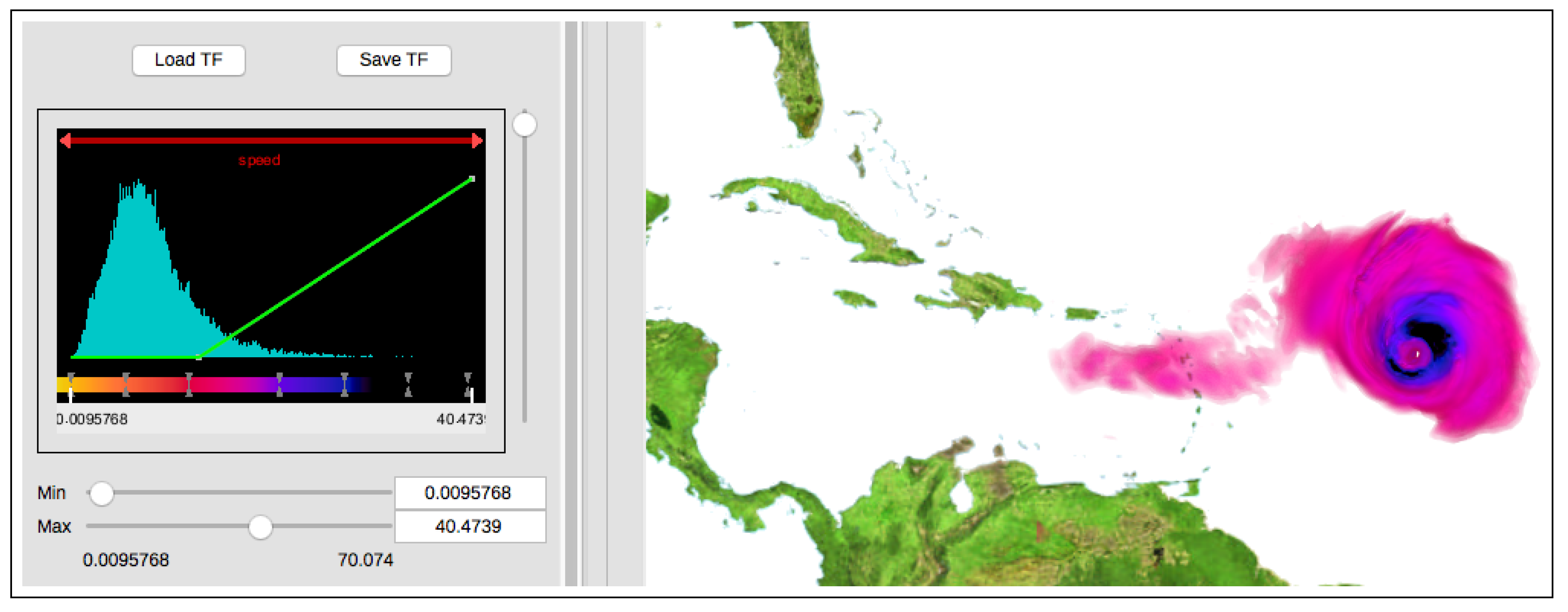
Figure 3 shows the interface of this widget. Data values represented in the histogram acquire the colors beneath them from the color palette. Line segments (in green) representing opacity are drawn on top of the histogram; users can use their mice to adjust existing segments or add and remove segments to achieve complex piecewise-linear shapes. In VAPOR’s transfer function editor, the higher a line segment is, the more opaque the data values under the line will be. Placing a line segment at the bottom of the histogram will result in values being fully transparent.
5.2. Slice Renderer
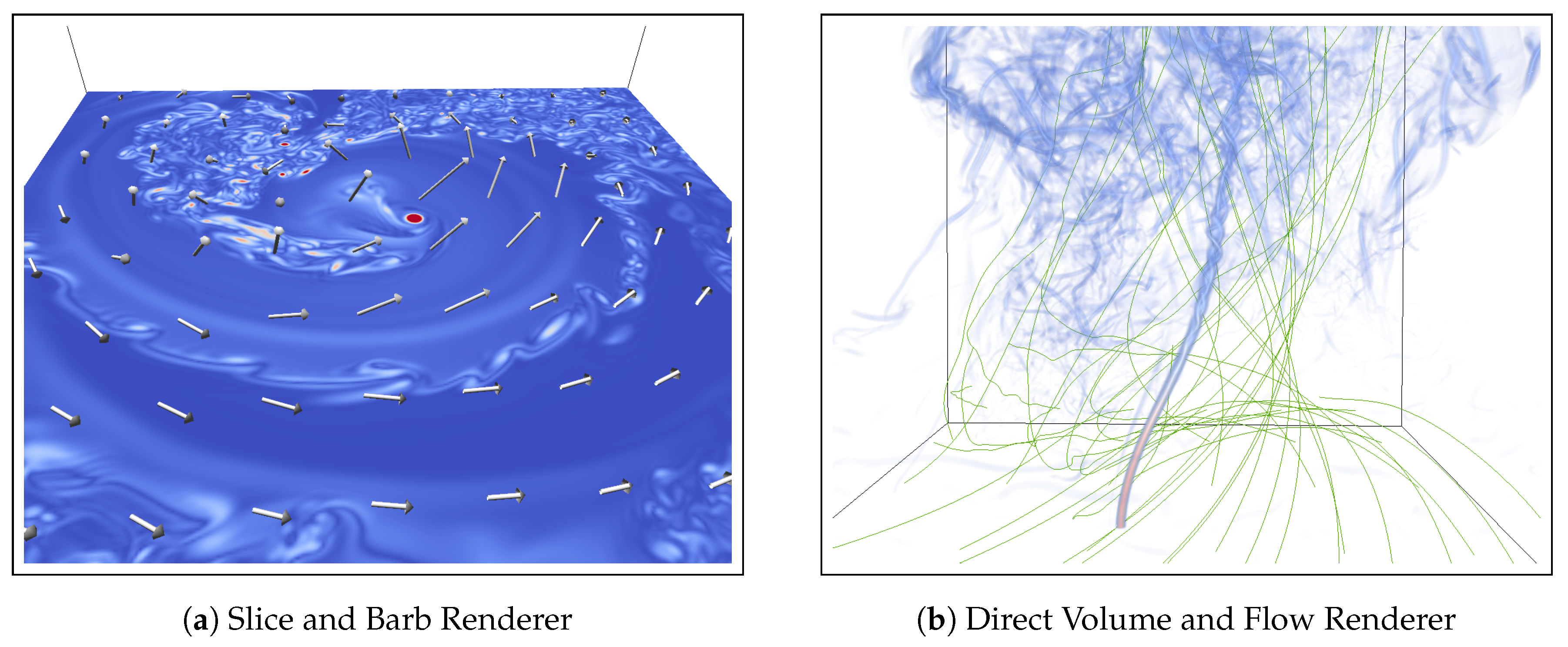
A Slice Renderer operates on 3D variables. It performs two tasks: (1) extracting a 2D data plane from the 3D data volume and (2) displaying this plane by mapping data values to colors via a user-defined transfer function. The extracted 2D data plane is currently constrained to be aligned to one of the three axes, providing a tomography-style examination. Values on the plane are interpolated from the volume using tri-linear interpolation. The Slice Renderer can interactively be positioned and oriented, providing a simple, efficient, and intuitive way to examine volumetric data.
Figure 4a illustrates a slice rendered perpendicular to the vortex core of a tornado, showing the location of the vortex core in red.
5.3. Direct Volume Renderer
The Direct Volume Renderer is the flagship renderer for 3D volumetric data. It is useful for both exploring the data as well as close-up examination of areas of interest. The Direct Volume Renderer achieves this by enabling the users to “see through” the volume, rendering only “interesting” areas of the data.
The Direct Volume Renderer mimics how the human eye sees a semi-transparent 3D object. More specifically, “rays” are emitted from the camera into the 3D volume, just like lines of sight from human eyes. These rays travel through the volume, sampling data values along the way, and accumulating colors and opacity at those samples. A ray stops traveling when either (1) it leaves the volume from the back or (2) it becomes completely opaque after accumulating sufficient opacity. This algorithm is often referred to as “ray casting” in the literature.
Using the transfer function editor, users usually assign opacity to only values of interest and leave other values completely transparent, revealing features inside of a 3D volume. Often, the renderings resemble natural phenomena, such as a cloud or a tornado. For example,
Figure 4b illustrates a volume rendering of vorticity magnitude from a tornado simulation. With only high vorticity areas being opaque, the vortex core of the tornado is clearly visible.
Figure 3 also illustrates a hurricane from volume rendering. More discussion on volume rendering in general can be found in this textbook [
39] and its optical models in this paper [
40].
VAPOR’s Direct Volume Renderer offers a few noteworthy characteristics:
OpenGL Shading Language (GLSL) implementation: GLSL is a low-level programming interface for Graphics Processing Units (GPUs), which means it is considerably more performant than higher-level GPU programming paradigms. GLSL is also an open standard and enjoys broad support from all major operating systems and GPU vendors, which means that this high performance is portable across three major operating systems (macOS, Linux, and Windows).
Separate algorithms optimized for regular and curvilinear grids: VAPOR implements two ray casting algorithms, one for regular and one for curvilinear grids. The algorithm for regular grids takes advantage of the regular grid structure, achieving very high performance. The algorithm for curvilinear grids adapts to the irregular geometry to produce correct renderings at the cost of less performance. To the best of our knowledge, VAPOR is the only visualization package in production use that supports curvilinear grids without expensive and error-prone resampling.
Support for missing values: VAPOR understands missing values that are common in ESS datasets and does not include them in color and opacity integration during ray casting.
Correct blending with other renderings: The semi-transparency in a volume rendering makes displaying multiple rendering outputs difficult. VAPOR’s Direct Volume Renderer takes into consideration the depth information of other renderings to blend them together correctly, so that the semi-transparent areas of a volume rendering will not obscure other renderings behind it.
Fast rendering mode: Maintaining interactivity requires high rendering performance, usually more than ten frames per second. VAPOR’s Direct Volume Renderer implements a “fast rendering” mode to accommodate this requirement. More specifically, a degraded rendering is produced during scene navigation (rotation, zoom, etc.), and a normal rendering is produced upon the completion of a sequence (e.g., when the scene rotation finishes). Fast rendering improves overall interactivity for compute-intensive operations such as volume rendering.
5.4. Isosurface Renderer
The Isosurface Renderer displays one or more surfaces in a 3D volume where the field exhibits a user-specified isovalue. Conceptually, it is the 3D generalization of 2D contour lines, representing points of a constant value within a region of space.
Isosurfaces in VAPOR are computed and rendered using the same basic machinery as direct volume rendering. The only difference is that a ray accumulates opacity only at isovalue locations, instead of integrating opacity along the entire ray. Isosurfaces allow examination of the volume in a more quantitative fashion than volume rendering, e.g., when one is interested in a specific data value. Another advantage of isosurfaces is the ability to color map a secondary variable on the isosurface, enabling the examination of two variables simultaneously. Finally, sharing the same code base in GLSL with the Direct Volume Renderer, the Isosurface Renderer has the same portable performance across platforms, flexible algorithm choices for regular and curvilinear grids, and support for fast rendering mode.
5.5. Flow Renderer
The Flow Renderer performs particle advection and then renders the resulting trajectories. In the advection step, the user first specifies a three-dimensional vector field, which is often velocity or magnetic fields. The user then specifies particle advection locations in both time and space, along with an advection stopping criterion. VAPOR treats these particles as massless and uses a Runge–Kutta fourth order method to perform advection on each particle, until the stopping criterion is met. The particle trajectories are rendered in the scene, with optional specifications such as rendering their partial or full lengths and coloring the trajectories based on a certain property.
Figure 4b illustrates flow rendering in a tornado simulation: particles were placed on the ground and can be seen to swirl around and move up the tornado.
VAPOR’s Flow Renderer supports a number of optional control parameters:
Steady or unsteady fields: The vector field can be steady (constant over time) or unsteady (varying with time).
Seed placement: Starting particle advection locations can be programmatically determined or be specified by the user using a list of seeding points. When seeds are programmatically placed, the placement can be uniform or randomly distributed within a user-specified region. Moreover, the random placement can be biased towards a selected variable’s value.
Advection direction: For steady fields, the particle advection direction can be forward, backward, or bi-directional.
Stopping criteria: The advection can be terminated based on a number of criteria such as leaving the domain, after a specified length of time, etc.
Coloring scheme: Advection trajectories can be colored by different schemes such as another variable or the length of the trajectory.
Save trajectories: Advection trajectories can be saved to a text file with the location and property values at each advection step.
5.6. Image Renderer
VAPOR can import GeoTIFF raster image files containing geo-referencing information and display the image in the same coordinate space as any geo-referenced data loaded into the application. The imagery and data will be correctly positioned within the scene.
Figure 3 illustrates a volume rendering of a hurricane on top of a geo-referenced map. VAPOR includes a set of high-resolution (500 m) global raster image maps from NASA’s Blue Marble Next Generation project [
41]. However, any image with proper geo-referencing information can be imported into VAPOR and displayed in the correct location. In fact, the image need not necessarily be a map; data plotted with another tool and stored as a GeoTIFF can be imported just as easily. Finally, with some limitations, VAPOR can export the rendered scene as a GeoTIFF that can then be imported into any tool that understands GeoTIFF imagery (e.g., Google Earth).
6. Use Case and Comparison
6.1. Background
VAPOR Version 2 was an invaluable resource for the visualization and analysis of tornado-producing thunderstorms in prior work [
42]. Experiences with VAPOR Version 2 in this research have driven some of the refactoring approaches for the VAPOR Version 3 code. Below, we present a case study conducted by co-author Orf with VAPOR Version 3 in recent simulations of tornado-producing thunderstorms at extremely high resolution.
In prior work [
42], results from a breakthrough simulation of a violently-tornadic supercell were presented. A newly-discovered feature dubbed the Streamwise Vorticity Current (SVC) was identified. The SVC is a helical tube of vorticity that begins with a primarily horizontal orientation that, over time, becomes more intense as it is tilted and drawn into the base of a strengthening thunderstorm updraft. The identification of the SVC was made with VAPOR Version 2 utilizing its volume rendering capabilities (
Figure 5). The scientific significance of this feature is reflected in the fact that an entire NSF sponsored field program recently was launched to detect it and other similar features in the atmosphere [
43].
One of the issues that provided friction for research use of VAPOR Version 2 was the requirement that all data be converted into the VDC format. CM1 output data in this research were saved in HDF5 format, spread amongst many files in a format the authors call “LOFS.” LOFS data were converted to a series of NetCDF files, each containing several 2D and 3D fields for a given model time. This was followed by the conversion of the NetCDF files to the VDC format, making data import an unwieldy two-step process.
6.2. Sources of Data for the Current Use Case
One of the notable features of VAPOR Version 3 is its ability to read CF-compliant NetCDF data natively [
25]. In our current use case, CF-compliant NetCDF files from a thunderstorm simulation were imported directly into VAPOR. In order to create CF-compliant data, modifications to the code that converts LOFS to NetCDF were made in order to provide the metadata required by VAPOR, such as the Cartesian coordinates of the mesh scaffolding the data. Following these simple modifications to the LOFS conversion code, CF-compliant NetCDF files were created in a single-step process from LOFS data, saving both time and disk space, as compared to the two-step process required in previous work. An additional advantage to the current approach is that CF-compliant NetCDF is a standardized format, so a single set of NetCDF files can be natively read by many useful analysis and visualization tools without any further conversions.
In the current use case, unprecedented high-resolution simulations of a tornado-producing thunderstorm needed to be visualized for presentation at an upcoming conference. The simulation, still unfinished at the time of the conference, utilized most of the Blue Water supercomputer, spanning over 1/4 trillion grid zones. Our goal was to present stills and animations that included the evolution of a devastatingly strong multiple vortex tornado that formed within the simulated thunderstorm.
Because the region involving the tornado is a small fraction of the full model domain, NetCDF files spanning only a subdomain were created. The visualization domain for the images shown in
Figure 6 spans 501 × 501 × 301 grid volumes (the full model simulation mesh contained 11,200 × 11,200 × 2000 cells; hence, the visualization volume contained only 0.03% of the volume spanned by the full simulation). The images in
Figure 6 are a tiny sampling of the total number of images created in this use case. For each of the images shown in this figure, several hundred model times, saved in 1-second intervals, were generated, in order to facilitate the creation of the animations. The following process was followed for creating a sequence of images in time:
Convert the whole LOFS data to disposable NetCDF files containing 2D horizontal data that are then viewed by the slice viewer ncview in order to choose the subdomain bounds desired for the CF-compliant NetCDF files to be input into VAPOR.
Using the same conversion program, convert LOFS data to CF-compliant NetCDF files spanning the desired subdomain volume.
Launch VAPOR on a Linux workstation, and then, import the group of sequentially-named NetCDF files.
Choose from 2D fields the desired surface 2D pseudocolor plot (we chose the vorticity or pressure trace at the surface that shows the path of the tornado and attendant suction vortices that leave a cycloidal path).
In this use case, volume rendering was used for 3D visualization. For each desired sequence of images, first select the colormap and opacity curves to achieve the desired visualization, and then, select the desired camera view.
Capture a sequence of images to PNG files. During this time, VAPOR steps through each time and visualizes/saves images. This process took roughly one hour per sequence utilizing a Radeon RX 580 graphics card.
Combine exported PNG files to a MP4 movie.
Each image in
Figure 6 represents a different view that highlights the features of a simulation that, to our knowledge, contains the highest resolution supercell tornado ever simulated at the time this article was drafted. The presentation of 2D surface swath data in conjunction with volume-rendered fields tells a compelling story, especially when animated, showing the path of dozens of subtornadic vortices moving with the storm, some of which converged together towards a central point that ultimately became the tornado. Such an information-rich presentation is instantly recognizable by domain scientists including field researchers who study tornadoes, and such visualizations have resulted in calling into question long-standing conceptual models involving tornado formation [
44]. Further, carefully-crafted volume-rendered visualizations involving the cloud and rain fields can easily be compared to photogrammetric observational data of real storms [
45,
46], validating the numerical model results.
6.3. Comparison with Other Visualization Packages
Compared to more generalized visualization packages such as VisIt and ParaView, VAPOR’s specialization allows it to simplify and streamline the process of analyzing and visualizing data in the ESS field. Specifically, VAPOR has out-of-the-box support for: (1) common ESS data formats including CF-compliant NetCDF, WRF, and MPAS; (2) missing value masks; and (3) common mapping projections in the ESS field. That said, VisIt and ParaView can still handle such cases, but they usually require a considerable amount of effort to perform data processing and/or conversion to register information from ESS data correctly (e.g., coordinates and missing values). The rest of this subsection uses two examples to illustrate this difference.
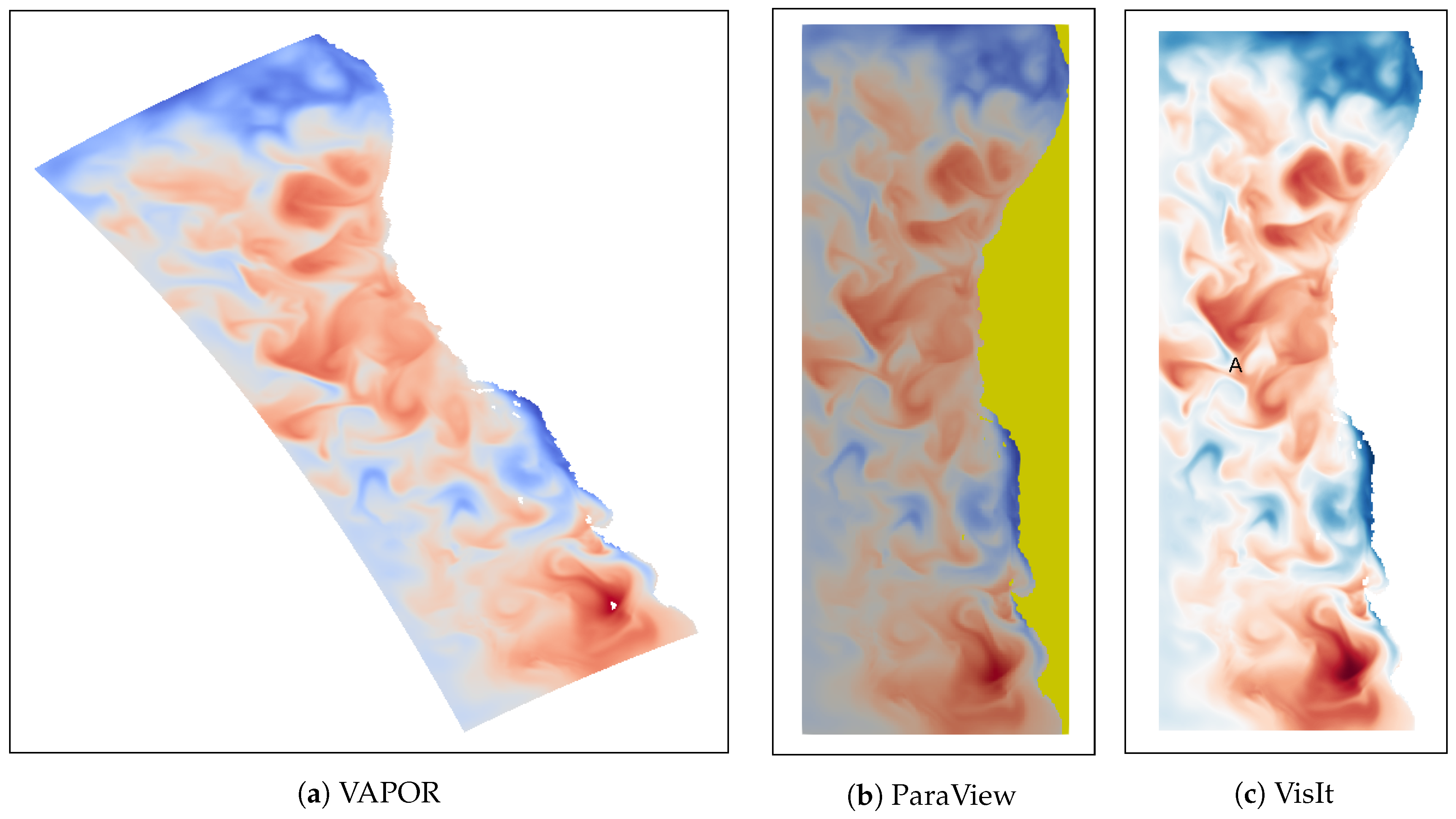
Figure 7 shows an out-of-the-box 2D pseudocolor rendering of an ocean simulation dataset using VAPOR, ParaView, and VisIt. The output of this simulation was stored as CF-compliant NetCDF files, which contain both curvilinear coordinates and missing data values. VAPOR produced a correct rendering, while both VisIt and ParaView failed to recognize the curvilinear coordinates, rendering the data on rectilinear grids. Furthermore, ParaView failed to recognize the missing data values, rendering them as a yellow block. We note that though it is possible to generate correct renderings using VisIt and ParaView by taking extra steps to process coordinates and missing values properly, VAPOR provided the most easy-to-use experience.
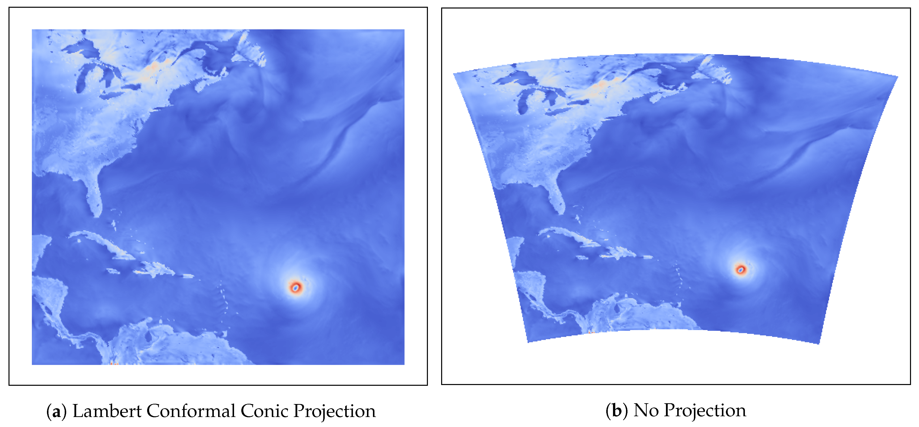
Figure 8 illustrates the effect of mapping projections on a 2D pseudocolor rendering from 2009’s Hurricane Bill simulation. The output of the simulation was stored in WRF format with the Lambert conformal conic projection. VAPOR automatically recognizes and applies the projection, rendering a square region. Without applying the projection, the same region would be rendered distorted. Correct mapping projection is especially important when multiple renderings from different datasets are blended in the same scene, in which case different datasets may use different projections. Again, we note that correct mapping projections are still possible in other applications through the use of plugins or scripting. However, VAPOR simply does the right thing without user intervention.
7. Discussion and Future Work
In this section we discuss some of our design choices in the development of VAPOR and lay out our immediate future work.
7.1. Design Choice Discussion
The software architecture described in
Section 3 is a major design shift over past VAPOR releases, and it has greatly reduced engineering effort and the chance of error during software development. A more detailed discussion was presented in
Section 3 (especially
Section 3.6); we only summarize here that it has received overwhelmingly positive feedback from the VAPOR development team.
The intensive use of modern OpenGL and its Shading Language (GLSL) is another big change from past VAPOR releases. While OpenGL has been evolving for more than twenty-five years, its release of Version 3.3 has introduced such significant changes that Version 3.3 and after are considered modern OpenGL, while versions prior to 3.3 are considered classic OpenGL. Among others, one of the most fundamental changes of modern OpenGL is that much of the computation from the classic OpenGL rendering pipeline is now performed by programmable shaders, which are written in GLSL and considered much more flexible and powerful.
VAPOR migrates its use of OpenGL from classic to modern (from Versions 2.3 to 4.1). This means we have not only re-written much of the rendering code using GLSL, but also implemented new algorithms that fit the programming model of GLSL (specifically, the ray casting algorithm in volume rendering and isosurface rendering). This decision turns out to be a double-edged sword. On the one hand, the more flexible nature of GLSL enables rapid algorithm development, and its unique programming model effectively harnesses the massive parallelism on GPUs, delivering very high performance. On the other hand, the reliability of GLSL programs heavily relies on the GPU drivers from GPU vendors, which can vary wildly across operating systems and GPU series. According to our tests, rendering failures are particularly more likely to occur with low-end GPU chips. These failures hurt the system portability of VAPOR (from high- to low-end systems), but will hopefully improve as vendors continue to release new drivers.
Lastly, a primary design goal of VAPOR is portable performance. This goal played a large role in choosing OpenGL to support rendering tasks. However, OpenGL and its shading language, GLSL, were designed primarily to support GPU rendering of simple geometric primitives (e.g., triangles). Tasks as complex as ray casting are arguably better suited to more general purpose programming environments. Unfortunately, such an environment for GPUs that is both considered mature enough for production applications and portable across GPU vendors does not yet exist. As an example, CUDA is probably most ready for production use, but it simply lacks platform portability. If such an environment does emerge in the future, the architectural changes made in the latest version of VAPOR should make it well positioned to migrate easily to a new programming model, perhaps one that, for example, more readily supports parallelization across multiple GPUs. Possible adoption of other programming interfaces will surely be revisited during future releases of VAPOR.
7.2. Future Work
While VAPOR is funded and developed primarily by NCAR, it is also an open-development project that is hosted on GitHub [
47]. Open development is a form of crowdsourcing that facilitates and embraces community involvement. One of its many benefits is the ability for users to download, build, and run the most current snapshot of the software at any point in time. Feedback and interactions with these early adopters improves the software’s usability, reliability, and correctness. The open development model also facilitates feature and functionality requests. However, perhaps most importantly, it enables direct community contributions to the code base in the form of bug fixes, code optimizations, feature improvements, and even new functionality. In other words, users have a strong ability to steer the direction of the project.
Based largely on community feedback, some of the more immediate priorities for the development team at NCAR include:
More parallelism: VAPOR can benefit from more parallelism in many of its compute-intensive calculations. Given the trend of recent parallel computing development, language directive-based schemes, such as OpenACC and OpenMP, are probably the best options for VAPOR.
CPU-based rendering engine: We plan to offer a CPU-based rendering engine as an alternative to the current OpenGL based one, hoping to render more reliably on low-end systems. Vendor-optimized toolkits, such as OSPRay from Intel, may be promising candidates.
Dedicated off-screen rendering buffer: Currently, VAPOR renders images to a window inside of the application user interface, meaning that the dimension of the final rendering is difficult to specify and often limited by the monitor size. Dedicating an off-screen rendering buffer would allow bigger and more flexible rendering dimensions.
Advanced wavelet codec: The VDC format could employ advanced wavelet codecs to improve its lossy compression efficiency and also eliminate the storage overhead discussed in
Section 4.3.4. SPECK [
48,
49], a codec that has demonstrated both high compression efficiency and relatively low computational cost, is under careful evaluation to be potentially included in VAPOR.
8. Conclusions
This paper has provided an overview of the latest iteration of VAPOR (Version 3), a cross-platform visualization package for data exploration in Earth System Sciences. It is a GUI-based desktop application that specifically provides ease of use in the ESS field with support for many numerical models and visualization renderers. Its visualization strength especially lies in the capability to render 3D volumetric data with a Direct Volume Renderer, Isosurface Renderer, and a Flow Renderer. VAPOR also uses various techniques to improve user interactivity, including a hierarchical data organization method and fast rendering modes in compute-intensive rendering processes. Version 3 of VAPOR has improved upon previous releases with a cleaner software architecture, a more organized user interface, and the capability to operate on computational grids commonly used in ESS directly. These improvements are aimed at increasing software extensibility and encourage open development from the ESS community. Finally, we demonstrated the usefulness of VAPOR by presenting a use case where VAPOR was used to visualize a simulated tornado and drive scientific discoveries.
Author Contributions
The VAPOR software is developed by J.C., S.P., S.L., and S.J. among others. The manuscript was drafted by S.L., and revised by all the coauthors. The use case in
Section 6 was provided by L.O.
Funding
Development of VAPOR is supported by the National Center for Atmospheric Research, which is a major facility sponsored by the National Science Foundation under Cooperative Agreement No. 1852977. Additional funding was provided in part through U.S. National Science Foundation grants 03-25934, 09-06379, 14-40412, a TeraGrid GIG award, and with support from the Korean Institute for Science and Technology Information (KISTI). Leigh Orf was supported by the Cooperative Institute for Meteorological Satellite Studies and National Science Foundation grants OAC-1614973, OAC-1663954, OAC-1550405, and AGS-1832327.
Acknowledgments
We thank Alan Norton, Kenny Gruchalla, Niklas Röber, Pamela Gillman, and many others for their contributions to the VAPOR software.
Conflicts of Interest
The authors declare no conflict of interest. The funders had no role in the design of the study; in the collection, analyses, or interpretation of data; in the writing of the manuscript, or in the decision to publish the results.
References
- Orbach, R.L. Computational Science: A Research Methodology for the 21st Century. In Proceedings of the American Physical Society March Meeting, Montreal, QC, Canada, 22–26 March 2004. s2.002. [Google Scholar]
- Johnson, C.; Moorhead, R.; Munzner, T.; Pfister, H.; Rheingans, P.; Yoo, T.S. NIH-NSF Visualization Research Challenges Report; IEEE Computing Society: Los Alamitos, CA, USA, 2006. [Google Scholar]
- Childs, H.; Brugger, E.; Whitlock, B.; Meredith, J.; Ahern, S.; Pugmire, D.; Biagas, K.; Miller, M.; Harrison, C.; Weber, G.H.; et al. VisIt: An End-User Tool For Visualizing and Analyzing Very Large Data. In High Performance Visualization—Enabling Extreme-Scale Scientific Insight; CRC Press: Boca Raton, FL, USA, 2012; pp. 357–372. [Google Scholar]
- Ahrens, J.; Geveci, B.; Law, C. Paraview: An end-user tool for large data visualization. In The Visualization Handbook; Elsevier: Burlington, MA, USA, 2005; p. 717. [Google Scholar]
- Clyne, J.; Rast, M. A prototype discovery environment for analyzing and visualizing terascale turbulent fluid flow simulations. Proc. Vis. Data Anal. 2005, 5669, 284–294. [Google Scholar]
- Clyne, J.; Mininni, P.; Norton, A.; Rast, M. Interactive desktop analysis of high resolution simulations: application to turbulent plume dynamics and current sheet formation. New J. Phys. 2007, 9, 301. [Google Scholar] [CrossRef]
- Upson, C.; Faulhaber, T.; Kamins, D.; Laidlaw, D.; Schlegel, D.; Vroom, J.; Gurwitz, R.; Van Dam, A. The application visualization system: A computational environment for scientific visualization. IEEE Comput. Graph. Appl. 1989, 9, 30–42. [Google Scholar] [CrossRef]
- Schroeder, W.J.; Lorensen, W.E.; Montanaro, G.; Volpe, C.R. VISAGE: An object-oriented scientific visualization system. In Proceedings of the 3rd Conference on Visualization, Boston, MA, USA, 19–23 October 1992; IEEE Computer Society Press: Los Alamitos, CA, USA, 1992; pp. 219–226. [Google Scholar]
- Doty, B.; Kinter, J., III. Geophysical Data Analysis and Visualization Using the Grid Analysis and Display System; Technical Report; National Aeronautics and Space Administration: Washington, DC, USA, 1995.
- Schroeder, W.J.; Lorensen, B.; Martin, K. The Visualization Toolkit: An Object-Oriented Approach to 3D Graphics; Kitware: New York, NY, USA, 2004. [Google Scholar]
- Wald, I.; Johnson, G.; Amstutz, J.; Brownlee, C.; Knoll, A.; Jeffers, J.; Gunther, J.; Navratil, P. OSPRay—A CPU Ray Tracing Framework for Scientific Visualization. IEEE Trans. Vis. Comput. Graph. 2017, 23, 931–940. [Google Scholar] [CrossRef] [PubMed]
- Nvidia. NVIDIA IndeX: 3D Visualization for Discovery and Exploration. Available online: https://developer.nvidia.com/index (accessed on 23 May 2019).
- The NCAR Command Language (Version 6.6.2) [Software]; UCAR/NCAR/CISL/TDD: Boulder, CO, USA, 2019. [CrossRef]
- Williams, D.N.; Doutriaux, C.M.; Drach, R.S.; McCoy, R.B. The flexible Climate Data Analysis Tools (CDAT) for multi-model climate simulation data. In Proceedings of the 2009 IEEE International Conference on Data Mining Workshops, Miami, FL, USA, 6 December 2009; pp. 254–261. [Google Scholar]
- May, R.; Arms, S.; Marsh, P.; Bruning, E.; Leeman, J. MetPy: A Python Package for Meteorological Data. Unidata 2017. [Google Scholar] [CrossRef]
- Met Office. A Powerful, Format-Agnostic, Community-Driven Python Library for Analysing and Visualising Earth Science Data. Available online: https://scitools.org.uk/iris/docs/latest/ (accessed on 23 August 2019).
- Arendt, A.A.; Hamman, J.; Rocklin, M.; Tan, A.; Fatland, D.R.; Joughin, J.; Gutmann, E.D.; Setiawan, L.; Henderson, S.T. Pangeo: Community tools for analysis of Earth Science Data in the Cloud. In Proceedings of the AGU Fall Meeting, Washington, DC, USA, 10–14 December 2018. [Google Scholar]
- Hoyer, S.; Hamman, J. xarray: ND labeled Arrays and Datasets in Python. J. Open Res. Softw. 2017, 5, 10. [Google Scholar] [CrossRef]
- Rocklin, M. Dask: Parallel computation with blocked algorithms and task scheduling. In Proceedings of the 14th Python in Science Conference, Austin, TX, USA, 6–12 July 2015; pp. 130–136. [Google Scholar]
- Hibbard, W.L.; Anderson, J.; Foster, I.; Paul, B.E.; Jacob, R.; Schafer, C.; Tyree, M.K. Exploring coupled atmosphere-ocean models using Vis5D. Int. J. Supercomput. Appl. High Perform. Comput. 1996, 10, 211–222. [Google Scholar] [CrossRef]
- Rautenhaus, M.; Kern, M.; Schäfler, A.; Westermann, R. Three-dimensional visualization of ensemble weather forecasts—Part 1: The visualization tool Met. 3D (version 1.0). Geosci. Model Dev. 2015, 8, 2329–2353. [Google Scholar] [CrossRef]
- Achtor, T.; Rink, T.; Whittaker, T.; Parker, D.; Santek, D. McIDAS-V: A powerful data analysis and visualization tool for multi and hyperspectral environmental satellite data. In Atmospheric and Environmental Remote Sensing Data Processing and Utilization IV: Readiness for GEOSS II; International Society for Optics and Photonics: Bellingham, WA, USA, 2008. [Google Scholar]
- Murray, D.; McWhirter, J.; Wier, S.; Emmerson, S. 13.2 The Integrated Data Viewer—A Web-Enabled Application for Scientific Analysis and Visualization. In Proceedings of the 19th International Conference on Interactive Information and Processing Systems for Meteorology, Oceanography, and Hydrology, Long Beach, CA, USA, 9–13 February 2003. [Google Scholar]
- Rautenhaus, M.; Böttinger, M.; Siemen, S.; Hoffman, R.; Kirby, R.M.; Mirzargar, M.; Röber, N.; Westermann, R. Visualization in meteorology—A survey of techniques and tools for data analysis tasks. IEEE Trans. Vis. Comput. Graph. 2018, 24, 3268–3296. [Google Scholar] [CrossRef] [PubMed]
- Eaton, B.; Gregory, J.; Drach, B.; Taylor, K.; Hankin, S.; Caron, J.; Signell, R.; Bentley, P.; Rappa, G.; Höck, H.; et al. NetCDF Climate and Forecast (CF) Metadata Conventions. Available online: http://cfconventions.org/cf-conventions/v1.6.0/cf-conventions.pdf (accessed on 23 August 2019).
- Skamarock, W.C.; Klemp, J.B.; Dudhia, J.; Gill, D.O.; Barker, D.M.; Wang, W.; Powers, J.G. A Description of the Advanced Research WRF Version 2; Technical Report; National Center for Atmospheric Research: Boulder, CO, USA, 2005. [Google Scholar]
- Skamarock, W.C.; Klemp, J.B.; Duda, M.G.; Fowler, L.D.; Park, S.H.; Ringler, T.D. A multiscale nonhydrostatic atmospheric model using centroidal Voronoi tesselations and C-grid staggering. Mon. Weather Rev. 2012, 140, 3090–3105. [Google Scholar] [CrossRef]
- Ringler, T.; Petersen, M.; Higdon, R.L.; Jacobsen, D.; Jones, P.W.; Maltrud, M. A multi-resolution approach to global ocean modeling. Ocean Model. 2013, 69, 211–232. [Google Scholar] [CrossRef]
- Morton, G.M. A Computer Oriented Geodetic Data Base and a New Technique in File Sequencing; International Business Machines Company: New York, NY, USA, 1966. [Google Scholar]
- Hilbert, D. Ueber die stetige Abbildung einer Line auf ein Flächenstück. Math. Ann. 1891, 38, 459–460. [Google Scholar] [CrossRef]
- Mallat, S.G. A theory for multiresolution signal decomposition: The wavelet representation. IEEE Trans. Pattern Anal. Mach. Intell. 1989, 11, 674–693. [Google Scholar] [CrossRef]
- Strang, G.; Nguyen, T. Wavelets and Filter Banks; Wellesley-Cambridge Press: Wellesley, MA, USA, 1996. [Google Scholar]
- Li, S.; Larsen, M.; Clyne, J.; Childs, H. Performance Impacts of In Situ Wavelet Compression on Scientific Simulations. In Proceedings of the In Situ Infrastructures for Enabling Extreme-Scale Analysis and Visualization Workshop, Denver, CO, USA, 12–17 November 2017; ACM: New York, NY, USA, 2017; pp. 37–41. [Google Scholar] [CrossRef]
- Li, S.; Marsaglia, N.; Garth, C.; Woodring, J.; Clyne, J.; Childs, H. Data Reduction Techniques for Simulation, Visualization and Data Analysis. Comput. Graph. Forum 2018, 37, 422–447. [Google Scholar] [CrossRef]
- Shneiderman, B. A grander goal: A thousand-fold increase in human capabilities. Educom Rev. 1997, 32, 4–10. [Google Scholar]
- Mininni, P.D.; Gómez, D.O.; Mahajan, S.M. Direct simulations of helical hall-mhd turbulence and dynamo action. Astrophys. J. 2005, 619, 1019. [Google Scholar] [CrossRef]
- Li, S.; Gruchalla, K.; Potter, K.; Clyne, J.; Childs, H. Evaluating the Efficacy of Wavelet Configurations on Turbulent-Flow Data. In Proceedings of the IEEE Symposium on Large Data Analysis and Visualization, Chicago, IL, USA, 25–26 October 2015; pp. 81–89. [Google Scholar] [CrossRef]
- Li, S.; Sane, S.; Orf, L.; Mininni, P.; Clyne, J.; Childs, H. Spatiotemporal Wavelet Compression for Visualization of Scientific Simulation Data. In Proceedings of the 2017 IEEE International Conference on Cluster Computing (CLUSTER), Honolulu, HI, USA, 5–8 September 2017; pp. 216–227. [Google Scholar] [CrossRef]
- Lichtenbelt, B.; Crane, R.; Naqvi, S. Introduction to Volume Rendering; Prentice-Hall, Inc.: Upper Saddle River, NJ, USA, 1998. [Google Scholar]
- Max, N. Optical models for direct volume rendering. IEEE Trans. Vis. Comput. Graph. 1995, 1, 99–108. [Google Scholar] [CrossRef] [Green Version]
- Stöckli, R.; Vermote, E.; Saleous, N.; Simmon, R.; Herring, D. The Blue Marble Next Generation—A True Color Earth Dataset Including Seasonal Dynamics from MODIS; NASA Earth Observatory: Greenbelt, MD, USA, 2005.
- Orf, L.; Wilhelmson, R.; Lee, B.; Finley, C.; Houston, A. Evolution of a Long-Track Violent Tornado within a Simulated Supercell. Bull. Am. Meteorol. Soc. 2017, 98, 45–68. [Google Scholar] [CrossRef]
- Tracking a Supercell Thunderstorm across the Great Plains. Available online: https://www.nsf.gov/discoveries/disc_summ.jsp?cntn_id=298179 (accessed on 15 July 2019).
- Orf, L. Petascale Supercell Thunderstorm Simulations and a New Hypothesis for Tornado Formation and Maintenance. Presented at the CSME-CFDSC Congress, London, ONT. Available online: https://youtu.be/5cel1fLxR04?t=2674 (accessed on 23 August 2019).
- Schyma, H.; Orf, L. Science inside a Tornado—Decoding the EF5. Video Documentary. Available online: https://youtu.be/e2wbn3ivHwc?t=646 (accessed on 23 August 2019).
- Schyma, H.; Orf, L. Tornado Science & Super Computers—Tornado Footage Compared with Simulations. Video Documentary. Available online: https://youtu.be/WFx9y4g9kNc?t=445 (accessed on 23 August 2019).
- VAPOR Is the Visualization and Analysis Platform for Ocean, Atmosphere, and Solar Researchers. Available online: https://github.com/NCAR/VAPOR (accessed on 23 August 2019).
- Islam, A.; Pearlman, W.A. Embedded and efficient low-complexity hierarchical image coder. In Electronic Imaging’98; International Society for Optics and Photonics: Bellingham, WA, USA, 1998; pp. 294–305. [Google Scholar]
- Tang, X.; Pearlman, W.A. Lossy-to-lossless block-based compression of hyperspectral volumetric data. In Proceedings of the International Conference on Image Processing (ICIP’04), Singapore, 24–27 October 2004; Volume 5, pp. 3283–3286. [Google Scholar]
Figure 1.
VAPOR software component diagram. The Control Executive marshals data and commands between the User Interface, and the other three primary components: Data Manager, Operators, and Renderers. The components in gray (Python and web) are still yet to be developed.
Figure 1.
VAPOR software component diagram. The Control Executive marshals data and commands between the User Interface, and the other three primary components: Data Manager, Operators, and Renderers. The components in gray (Python and web) are still yet to be developed.
Figure 2.
Volume rendering of a high-vorticity area in a turbulent flow. Different subfigures are generated using different versions of the same data. These versions differ in resolutions (Res) and lossy compression ratios (Comp), as noted in the subcaptions. (a) represents the ground truth rendering from the original data.
Figure 3.
A screenshot of VAPOR. The left panel shows the interface of a transfer function editor, and the right panel shows a visualization of a simulation of 2009’s Hurricane Bill in the Caribbean sea of the Atlantic. The visualization is a volume rendering of the horizontal wind speed of Bill on top of an image rendering of the Earth in the same region. The transfer function specified on the left is applied to the volume rendering (but not image rendering) on the right.
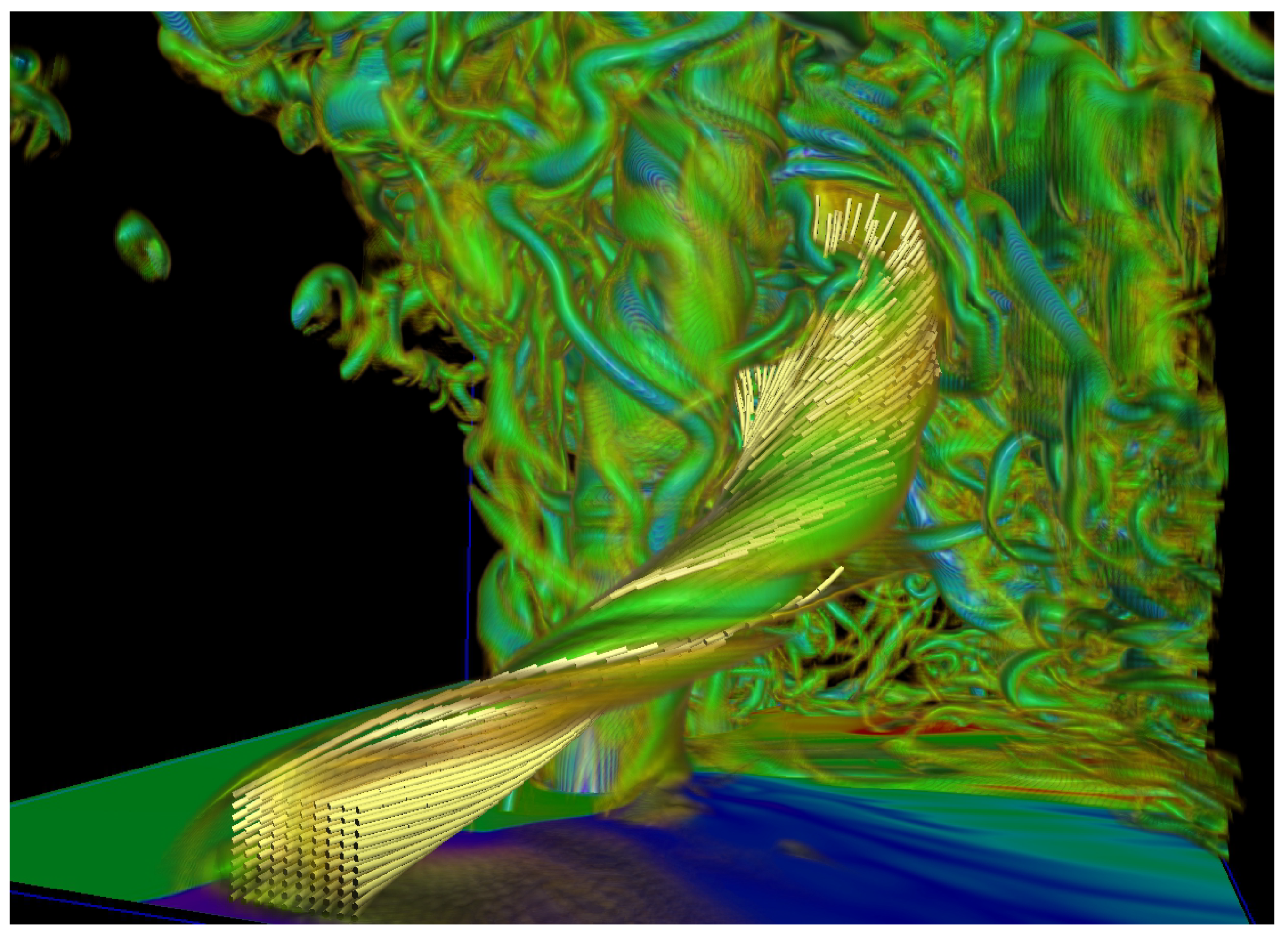
Figure 4.
Showcase of four renderers. (a) A tomography style slice in perpendicular to the vortex core of a tornado and a group of barbs showing the wind direction. The slice is of variable cloud liquid water (qcloud), and the barbs are of the wind velocity. (b) A volume rendering of the vorticity magnitude showing the vortex core of a tornado and a group of flow lines (in green) of velocity showing trajectories of particles being advected by the tornado.
Figure 5.
VAPOR Version 2 volume rendering of the 3D vorticity field and air trajectories calculated using the unsteady flow option from a simulation conducted in the year of 2014. The tube of vorticity that is embedded with trajectories was dubbed the streamwise vorticity current and is a feature of significant interest in the field of mesoscale meteorology.
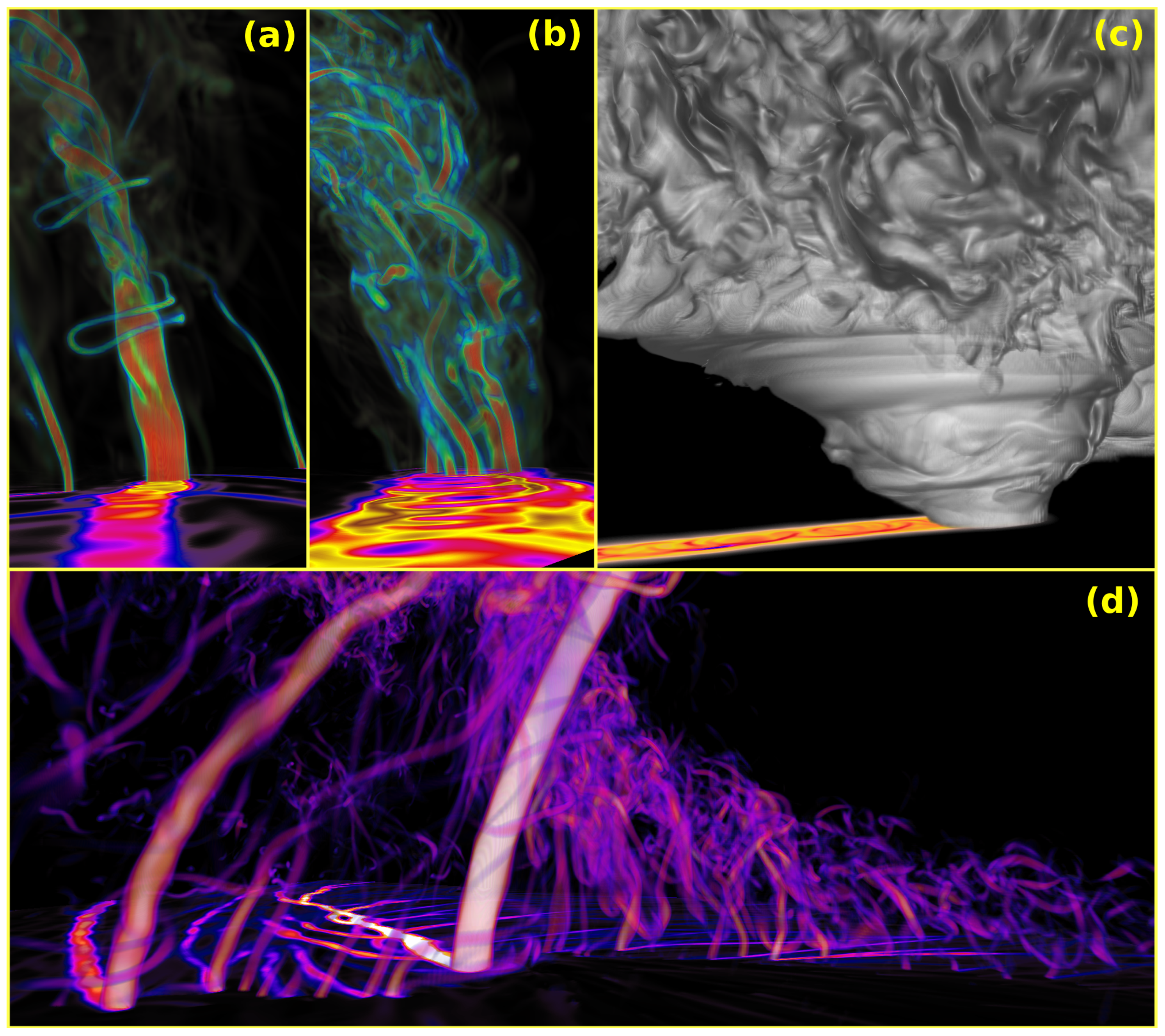
Figure 6.
Imagery created with VAPOR Version 3 of a 10-m supercell simulation. (a) Volume-rendered cyclonic vertical vorticity, highlighting the 3D structure of the tornado shortly after formation. The 2D surface field traces the maximum surface cyclonic vertical vorticity, providing a representation of the tornado’s path. The view is following the tornado’s path. (b) Same as in (a), but later in the simulation when the tornado exhibits a multiple vortex structure. (c) Volume-rendered cloud mixing ratio, with parameters chosen to present a quasi-photorealistic view of the cloud field. The 2D surface field traces the minimum pressure found in the tornado’s path. (d) Same as in (a,b), but a different, wider view and utilizing different opacity and colormap choices. The vortex to the left, which merges with the tornado later in the simulation, is weaker than the nascent tornado, as evidenced by the vortex’s more transparent and darker visual presentation and path.
Figure 7.
2D pseudocolor rendering of an ocean simulation off the west coast of North America using three visualization packages and their default settings. The rendered variable is surface net heat flux (shflux), and the data are in CF-compliant NetCDF format.
Figure 7.
2D pseudocolor rendering of an ocean simulation off the west coast of North America using three visualization packages and their default settings. The rendered variable is surface net heat flux (shflux), and the data are in CF-compliant NetCDF format.
Figure 8.
2D pseudocolor rendering of 2009’s Hurricane Bill simulation using VAPOR with Lambert conformal conic projection enabled (a) and disabled (b). The rendered variable is friction velocity (UST), and the data are in WRF format.
Figure 8.
2D pseudocolor rendering of 2009’s Hurricane Bill simulation using VAPOR with Lambert conformal conic projection enabled (a) and disabled (b). The rendered variable is friction velocity (UST), and the data are in WRF format.
Table 1.
Test system specifications.
Table 1.
Test system specifications.
| CPU: | Intel Core-i7 (quad-core, 3.6 GHz) |
| GPU: | Nvidia GeForce GTX 1060 |
| Memory: | 32 GB |
| OS: | Ubuntu 16.04 |
Table 2.
Frames-per-second on different data resolutions (column) and 3D renderers (row).
Table 2.
Frames-per-second on different data resolutions (column) and 3D renderers (row).
| Resolution | 1283 | 2563 | 5123 | 10243 |
| Volume | 25.15 | 20.88 | 4.42 | 0.26 |
| Isosurface | 92.86 | 83.64 | 27.13 | 0.27 |
Table 3.
Timing of VAPOR to prepare data in VDC format and reconstruct back to gridded data.
Table 3.
Timing of VAPOR to prepare data in VDC format and reconstruct back to gridded data.
| | Prepare | Reconstruct |
|---|
| Resolution | 10243 | 10243 | 5123 | 2563 |
| Second | 107.93 | 22.11 | 16.03 | 15.53 |
Table 4.
Actual storage size and overhead in percentage of the VDC format at different lossy compression ratios. Overhead is compared against the target compression ratio.
Table 4.
Actual storage size and overhead in percentage of the VDC format at different lossy compression ratios. Overhead is compared against the target compression ratio.
| | Original | VAPOR Format |
|---|
| Ratio | N/A | 1:1 | 10:1 | 100:1 | 500:1 |
| Size (MB) | 4295 | 4617.1 | 751.64 | 75.17 | 15.04 |
| Overhead | N/A | 7.5% | 75.0% | 75.0% | 75.1% |
© 2019 by the authors. Licensee MDPI, Basel, Switzerland. This article is an open access article distributed under the terms and conditions of the Creative Commons Attribution (CC BY) license (http://creativecommons.org/licenses/by/4.0/).


