1. Introduction
The El Niño-Southern Oscillation (ENSO), which is the most important driver of interannual variability, can cause climate changes and trigger disasters all across the globe [
1]. The El Niño (EN) in 2015–2016 was indeed a strong event, with dramatic impacts on a global scale. The warm sea surface temperature anomaly (SSTA) started to strengthen in the boreal spring and early summer of 2015, and the strongest EN event finally materialized in the boreal winter of 2015–2016 [
2,
3]. Moreover, due to the unusual heat in the equatorial Pacific in the early spring of 2014, this EN can be seen as one of the longest ENs due to the mutual influences of long-term climate change and the strong EN. This EN lasted for 21 months and spanned two years, (from the summer of 2014 to the spring of 2016) [
4]. It showed not only the features of all strong ENs, but also some distinct characteristics different from past extreme ENs [
5,
6,
7,
8,
9]. Thus, the further study of the ENSO and its complex behaviors is helpful. In this study, a comparison of this ENSO event with recent other ENSO events was carried out. The study is of great importance for improving ENSO prediction and obtaining a better understanding of the nature and dynamic mechanisms of the ENSO.
In recent years, several studies have suggested that ENSO behaviors are becoming more and more complex, including their spatial distribution and intensity [
10,
11]. The evolution of the 2015/2016 EN showed unusual complexity, and its performance may have involved the interaction of decadal variability and global warming [
12]. However, the current research on the 2015/2016 EN, including the processes associated with the warming anomaly present during 2014–2015, are still not understood well [
13,
14,
15,
16,
17,
18,
19]. Therefore, this has led scientists to investigate the recent ENSO events. Several relevant questions need to be answered: What factors enhanced the warming event in 2015–2016? What hindered the EN pattern during the boreal summer of 2014? Why were there apparent differences in the related physics between the 2014/2016 ENs and recent ENs? Moreover, are there any reliable early signals for predicting EN and its intensity?
It is widely agreed that salinity is an important component of the fundamental ocean state. Moreover, salinity can, in turn, indirectly affect ocean temperature through modulating the oceanic density fields [
20,
21,
22]. Lukas and Lindstrom [
23] demonstrated that the ocean density associated with salinity affects the stability of upper ocean stratification, leading to the change of barrier layer thickness (BLT) in the western Pacific. Furthermore, the barrier layer (BL) can suppress/enhance the vertical mixing and entrainment from below into the upper ocean, playing a role in modulating the sea surface temperature (SST) [
24]. Recently, Zheng and Zhang [
25] have highlighted the salinity contribution to modulating ENSO evolution through affecting the interannual anomalies of stratification in the western-central equatorial Pacific. For example, during the 2007/2008 La Niña, a positive sea surface salinity anomaly (SSSA) in the western-central equatorial Pacific resulted in the destabilization of the upper ocean by increasing oceanic density, then cooling the SST. The coupled analyses confirmed that BL is essential for modulating the upper ocean heat accumulation for ENSO evolution in the western equatorial Pacific [
24]. Moreover, Zhu et al. [
26] pointed out that the salinity anomaly in the ocean thermal structure is a precursor for ENSO. The comparison of the substantial formations of and evolution between the 1997/1998 EN and the 2014/2016 EN showed that the 2015/2016 EN presented obvious SSSA patterns associated with ENs [
27]. Meanwhile, the SSSA of the 2015/2016 EN were characterized by a strong precipitation anomaly in the western Pacific [
28]. However, the role of salinity and the related BL during the 2015/2016 EN have not been fully investigated.
This study focuses on the oceanic physics associated with salinity and the effects of salinity on recent strong ENs, especially the strongest EN during 2015–2016. Based on the relationship among variations of SST, the salinity anomaly, and the salinity-related physical fields, this paper explores the dominant mechanisms driving SSSA, to further examine the relationship between salinity variability and EN, and to find the possible driving forces of ENs in the equatorial Pacific. The analyses included the following two objectives: (1) To identify the relationships among the SSTA, sea surface salinity (SSS) variability, and salinity effects on EN; (2) To determine the possible physical mechanism of the salinity anomaly. The structure of this paper is as follows: A brief introduction describes the data and methods involved in
Section 2;
Section 3 shows the spatial-temporal structures, evolution of oceanic conditions, SSTA, and sea salinity using spatial-temporal variations;
Section 4 analyzes and compares the characteristics of salinity and the related ocean physics during the three ENs;
Section 5 further discusses the effect of interannual salinity variations on SSTA by effects on BLT;
Section 6 details analyses of the relationship between the salinity variability and the related physics anomalies during the three ENs, and discusses the possible mechanism of salinity variation through the salinity balance; finally, some remarks and a discussion of the findings are presented in
Section 7.
2. Data and Methods
In this paper, the gridded ocean three-dimensional salinity and temperature data were obtained from the Array for Real-Time Geostrophic Oceanography (ARGO) and the Simple Ocean Data Assimilation (SODA) reanalysis dataset, respectively. ARGO data were provided from the processed monthly data obtained from the International Pacific Research Center/the Asia-Pacific Data-Research Center. These monthly data have been produced since 2005 by optimal interpolation, with a spatial resolution of 1° × 1° from a depth of 5 to 2000 m. SODA version 3.3.1 data are produced by an ocean reanalysis system with the 0.5° × 0.5° spatial resolution and a 40-level depth resolution from Jan. 1980 to Dec. 2015. A more comprehensive description is provided in Carton and Giese [
29].
Additional data used include precipitation data since January 1979 obtained from the Global Precipitation Climatology Project (GPCP) dataset (version 2) with a spatial resolution of 2.5° × 2.5° [
30]. The monthly gridded evaporation data are from the Objectively Analyzed Ocean-Air Fluxes (OAFlux) dataset [
31] for the global oceans since 1958, with 1.0° × 1.0° resolution.
In this study, the mixed layer depth (MLD) and isothermal layer depth (ILD) were identified based on three-dimensional salinity and temperature. The ILD was calculated as the depth where the temperature was lower than that at the 10 m depth, and ΔT = 0.2 °C. The MLD is the depth where the density difference (Δρ) is higher than that at 10 m, and in which the Δρ is equal to the corresponding temperature difference of 0.2 °C [
32,
33]. When the MLD is shallower than the ILD, the difference between the MLD and ILD (ILD minus MLD) is defined as the BLT [
34,
35].
Referring to Zheng and Zhang [
25], the following analysis was used to diagnose the contributions of temperature and salinity to BLT during an ENSO event. Based on the above definition, a field is denoted as BLT (T, S), which can be attributed to temperature and/or salinity. Then, the contribution can be determined for the field of interest using temperature and salinity fields (
Table 1).
Additionally, the salinity tendency in the mixed layer can be calculated by the surface forcing, surface advection, and subsurface effect at the interannual scale, in the equatorial Pacific [
36,
37,
38]. Note that in this paper, due to the location of the study region in the tropical Pacific, the fresh water flux (FWF: evaporation (E) minus precipitation (P)) associated with surface forcing was defined as a primary factor dominating surface forcing, in terms of salinity budgets. The role of these processes in the changes of observed mixed layer salinity was calculated by using available datasets.
3. Spatial and Temporal Evolutions of SSTA and SSSA during the Three ENs
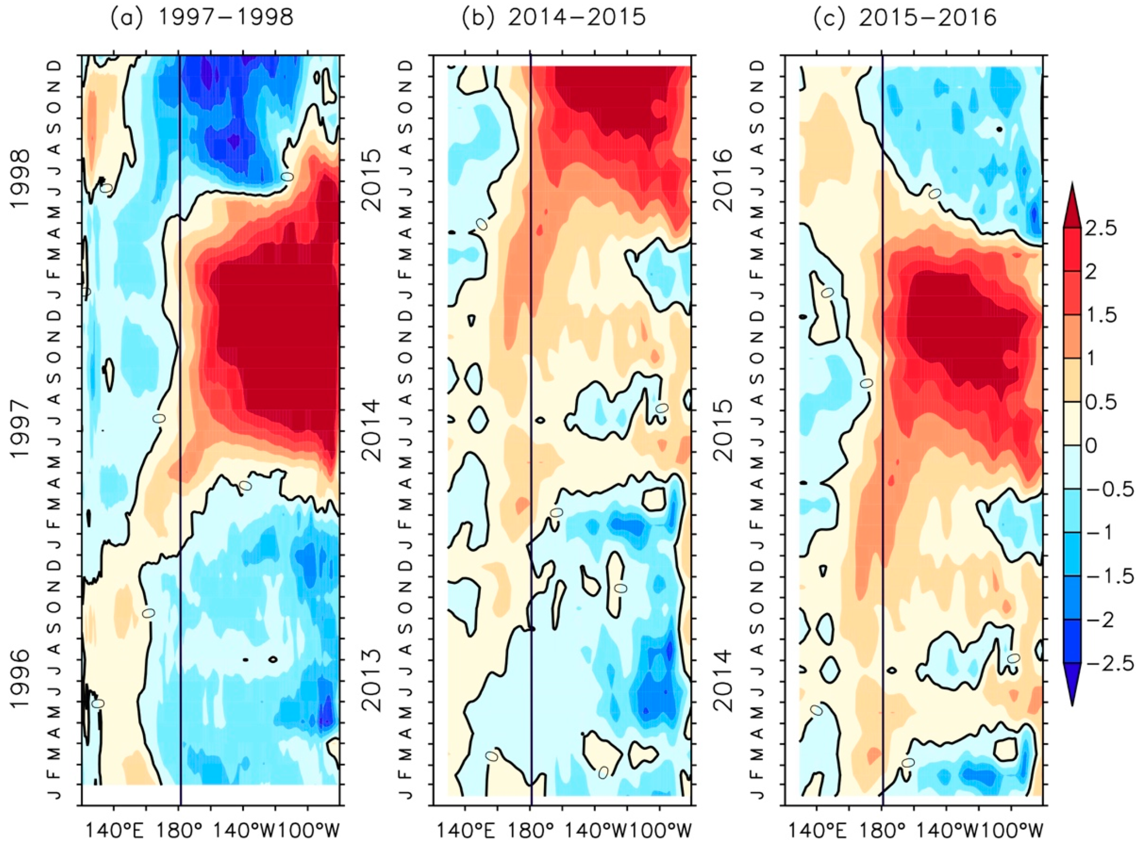
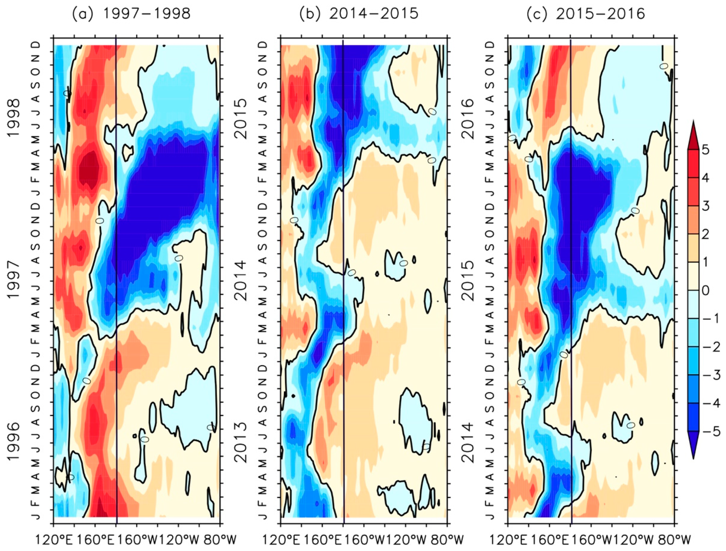
Figure 1 shows the spatial and temporal evolution of SSTA during the ENs in 1997/1998, 2014/2015 and 2015/2016 in the equatorial Pacific. It is known that the 1997/1998 and 2015/2016 ENs are two of the extreme events on record, while 2014/2015 was a weak EN (
http://www.pmel.noaa.gov/tao/elNiño/wwv). As can be seen, during the 1997/1998 and 2015/2016 ENs, a positive SSTA appears near the dateline in the central equatorial Pacific and the eastern equatorial Pacific, by April of each of the EN years, respectively (
Figure 1a–c). In the eastern equatorial Pacific, the SSTA continues to extend westward stably, and the intensity increases rapidly to more than 2.5 °C in the following two months. Then, the strong positive SSTA moves across 180° in the central Pacific, steadily increasing until April of the following year. In contrast, during the 2014/2015 EN, a positive SSTA is observed to the west of the dateline in February 2014 in the equatorial eastern Pacific. Subsequently, the warm SSTA continues to strengthen until June 2014; however, a transition of SSTA (i.e., from increase to decrease) occurred from June 2014 (
Figure 1b). Furthermore, it is interesting to note that in October 2014, another anomalous warming event occupies the eastern equatorial Pacific, which can be considered as the early period warming anomaly of the 2015/2016 EN. Therefore, this strong EN predicted by various scientific research institutions terminates immediately [
39]. Until November 2014, the SST west of the dateline warms up again and slowly moves eastward. Then, the positive SSTA in the eastern equatorial Pacific rebounds more than 2 °C in April of 2015, and slowly extends westward until April of 2016.
In addition, comparing the strong ENs with the weak EN, the dates of positive SSTAs (>1 °C) show a marked difference in the western-central equatorial Pacific. For example, both the strong ENs in 1997/1998 and 2015/2016 start with a warm SSTA, which develops rapidly and exhibits an unprecedented evolution process, with a strong SSTA more concentrated in the western-central Pacific. However, the intensity of the 2015/2016 EN is slightly weaker than that of the 1997/1998 EN in the Niño3 region. In contrast to the strong ENs, although the 2014/2015 EN shows a warming SSTA in the western-central equatorial Pacific from the winter to the summer of 2014, it evolves rapidly only after the spring of 2015. Note that the occurrence of the 2014/2015 weak EN led to an increased intensity for the 2015/2016 EN, in association with the Niño4 SSTA. The weak warming process in 2014/2015 is widely believed to have played an important role in maintaining the strong 2015/2016 EN. In addition, its different spatial pattern with respect to previous ENs may also be attributed to the potential mechanism related to this weak EN [
9,
39].
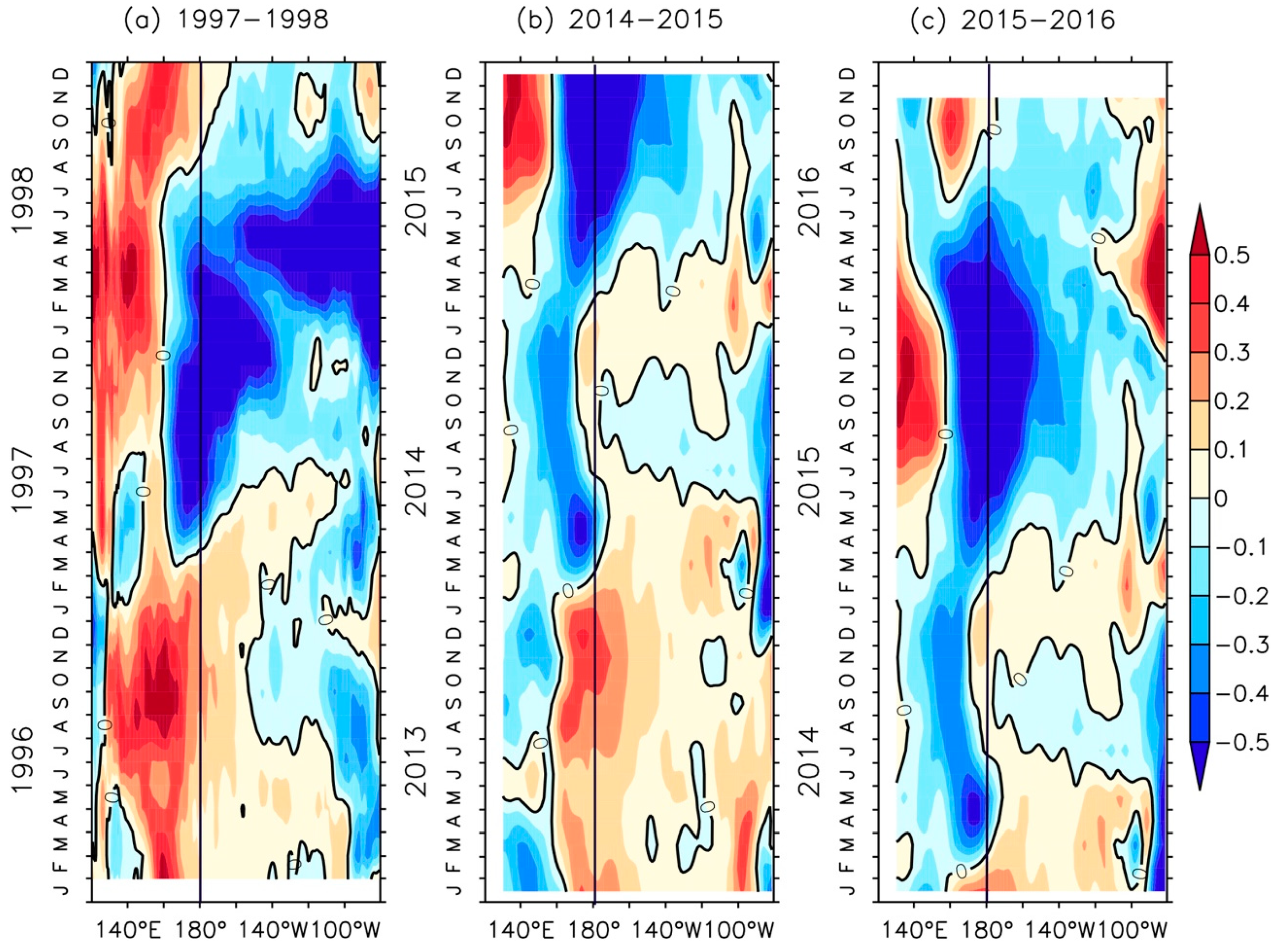
As one of the basic ocean variables, salinity influences vertical heat transfer between different layers by affecting ocean density and stratification. Salinity plays an important role in ENSO evolution [
40]. In order to describe the SSSA corresponding to the SSTA details during ENs, the spatial and temporal evolution of the SSSA during the three ENs is shown in
Figure 2. It was found that in the spring (the pre-period of EN) of 1997, 2014, and 2016, strong negative SSSAs appeared near the dateline in the equatorial Pacific, during which negative SSSAs maintained the peak of above −0.5 psu. For example, in April 1997, a strong negative SSSA appears to the west of the dateline, and the negative anomaly rapidly increases in intensity and slowly extends to the equatorial eastern-central Pacific, as seen in
Figure 2a. Similarly, during the pre-period of the 2015/2016 EN, though a continuous weak positive SSSA is stably maintained in the warm pool (WP), a negative SSSA rapidly extends eastward along the equator with a quickly increasing intensity, within the 160° E–160° W box in the equatorial Pacific in April (
Figure 2c). For the two strong ENs, the evolution of the SSSA near the dateline is generally similar, in which the negative SSSA develops and extends eastward from the WP in the early period. The negative SSSA in the 2015/2016 EN persists longer than that in 1997–1998.
However, for the 2014/2015 EN, the SSSA presents a different feature in its evolution. Before the EN, there was no significantly increasing and eastward-moving negative SSSA, corresponding to the weak positive SSTA in the east edge of WP (
Figure 2b). In the winter of 2013, the SSSA in the equatorial eastern Pacific shows similar characteristics as the 1997/1998 EN in 1996, but a significant negative anomaly appears and lasts throughout 2014. After appearing to the west of the dateline in the spring of 2014, the strong negative SSSA does not develop or move eastward in the summer, inconsistent with other strong ENs. On the contrary, its intensity weakened, and it slowly shifted westward, which led to a slight salinity change near the dateline from the summer of 2014 to the spring of 2015.
Moreover, the WP convergence area near the dateline in the equatorial Pacific is characterized by a complex thermohaline structure, which is the main area responsible for ENs occurring and developing [
41]. Strong salinity fronts in this region are closely related to SSSA and SSTA variations, affecting the occurrence and development of ENs. Therefore, temperature and salinity variations in this region often serve as a precursor to the ENSO [
42,
43,
44,
45]. During the evolutions of the three ENs, the SSSAs show distinct regional characteristics, with obvious zonal displacement of the negative SSSA west of the dateline showing, as with the SSTA. In general, ocean salinity, along with temperature, is not only a component of the sea water state equation but is also a passive tracer of ocean dynamics. During the three ENs, the SSS shows relatively obvious contemporaneous or even early changes, especially near the dateline. During evolution of the EN, a significant negative SSSA appears in the western equatorial Pacific, which corresponds to the positive SSTA (
Figure 1), and the negative SSSA lasts until the warming weakens and disappears. As seen for the two strong ENs, the negative SSSA in 2015 is significantly smaller, and is located west of that in 1997, which is consistent with the different spatial distributions of the corresponding SSTA. The termination of the SST warming in 2014–2015 also corresponds to the stagnation process of the negative-changing SSSA.
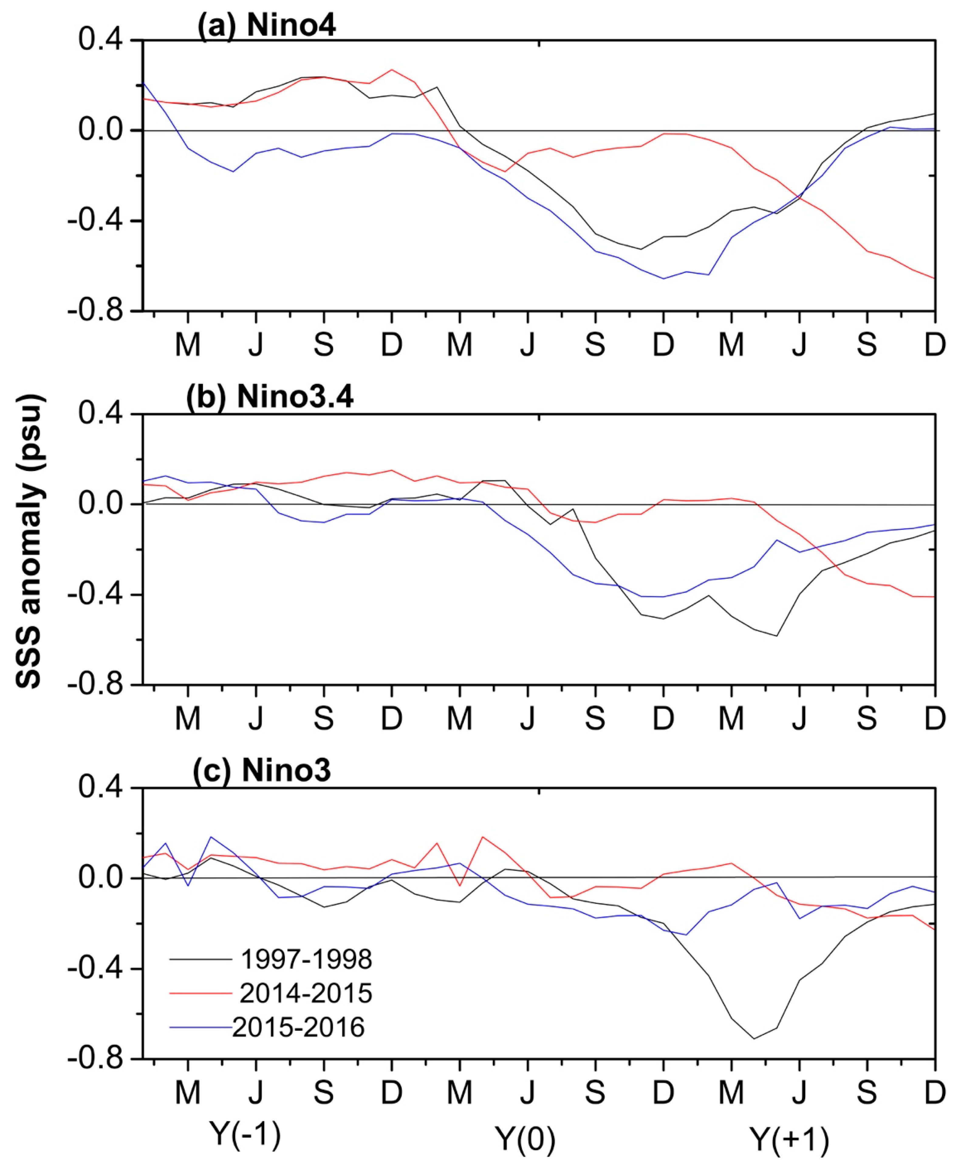
Figure 3 shows the development of area-averaged SSSAs in three special regions—the Niño 3.4, Niño 3, and Niño 4 regions—to more clearly describe ocean salinity variability along the equator during ENs, and to further quantitatively analyze the zonal shift of SSSA along the equator. According to the regional characteristics of the SSSA during ENs, the Niño4 area-averaged SSSA more obviously reflects the evolution characteristics of the SSSA over the western-central equatorial Pacific near the dateline during ENs. As seen in
Figure 3a, the negative SSSA in the Niño 4 region increases significantly from the spring of the EN occurrence year and reaches a peak in November–December during the 1997/1998 EN and the 2015/2016 EN, respectively. The evolutions of negative SSSAs during the two strong ENs are relatively consistent. As the negative SSSA lasts for a long time in the Niño4 region in 2015, the negative SSSA peak in the Niño4 region in 2015–2016 is higher than that in 1997–1998. By contrast, the SSSA in the 2014/2015 EN shows significant differences from those during the two strong ENs. The positive SSSA exists continuously from 2013 to the spring of 2014, then begins to decrease rapidly and becomes a negative anomaly. Although the SSSA in the 2014/2015 EN is similar to the early performance of SSS variations in the 1997/1998 EN, which lasts only two months after the negative SSSA increases and reaches a peak of 0.2 psu, the negative SSSA then slowly returns to a normal state after the winter of 2014. In addition, compared with SSSA evolutions in the Niño3.4 and Niño 3 regions, the negative SSSAs in Niño 3.4, Niño 3, and Niño 4 regions of 2014 increase first and decrease later, but do not continue to develop as SSSAs during the period of the strong ENs.
4. Ocean Physics Associated with Salinity during the ENSO
The physics of the mixing layer and barrier layer are key to the way in which salinity affects the thermodynamic process of the ocean. In recent years, a large number of observation and simulation studies have validated the finding that weak/strong vertical heat transfer increases/reduces heat accumulation in the upper ocean, thereby warming/cooling the SST [
46]. For example, Zheng and Zhang [
25] found that during the 2007/2008 La Niña, a positive SSSA in the western-central Pacific acted to destabilize the upper ocean and deepen the mixed layer (ML), which further enhanced the negative SSTA associated with the La Niña event. Meanwhile, according to the definition of the BL, the difference between MLD and ILD determines the BLT. Salinity plays an essential role in determining the BLT via modulating the MLD. With the aid of a coupling model, Maes et al. [
24] proved that the absence of the BL can cause more obvious mixing and entrainment effects between sea layers; hence, as they pointed out, if the effect of the BL is removed from the model, EN may weaken, suspend, or even not occur [
24,
47,
48]. Therefore, the BL is important for the occurrence and evolution of the ENSO.
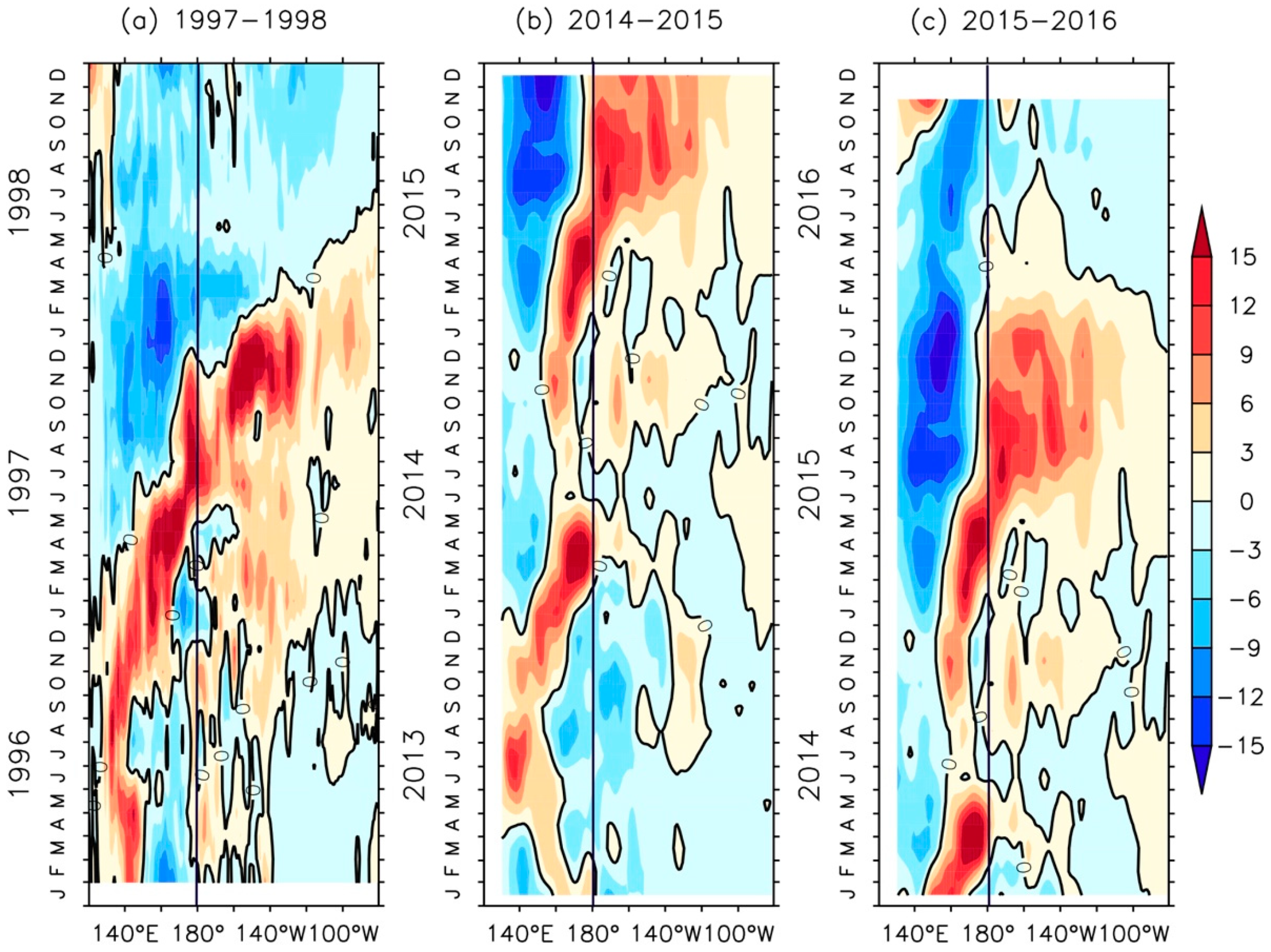
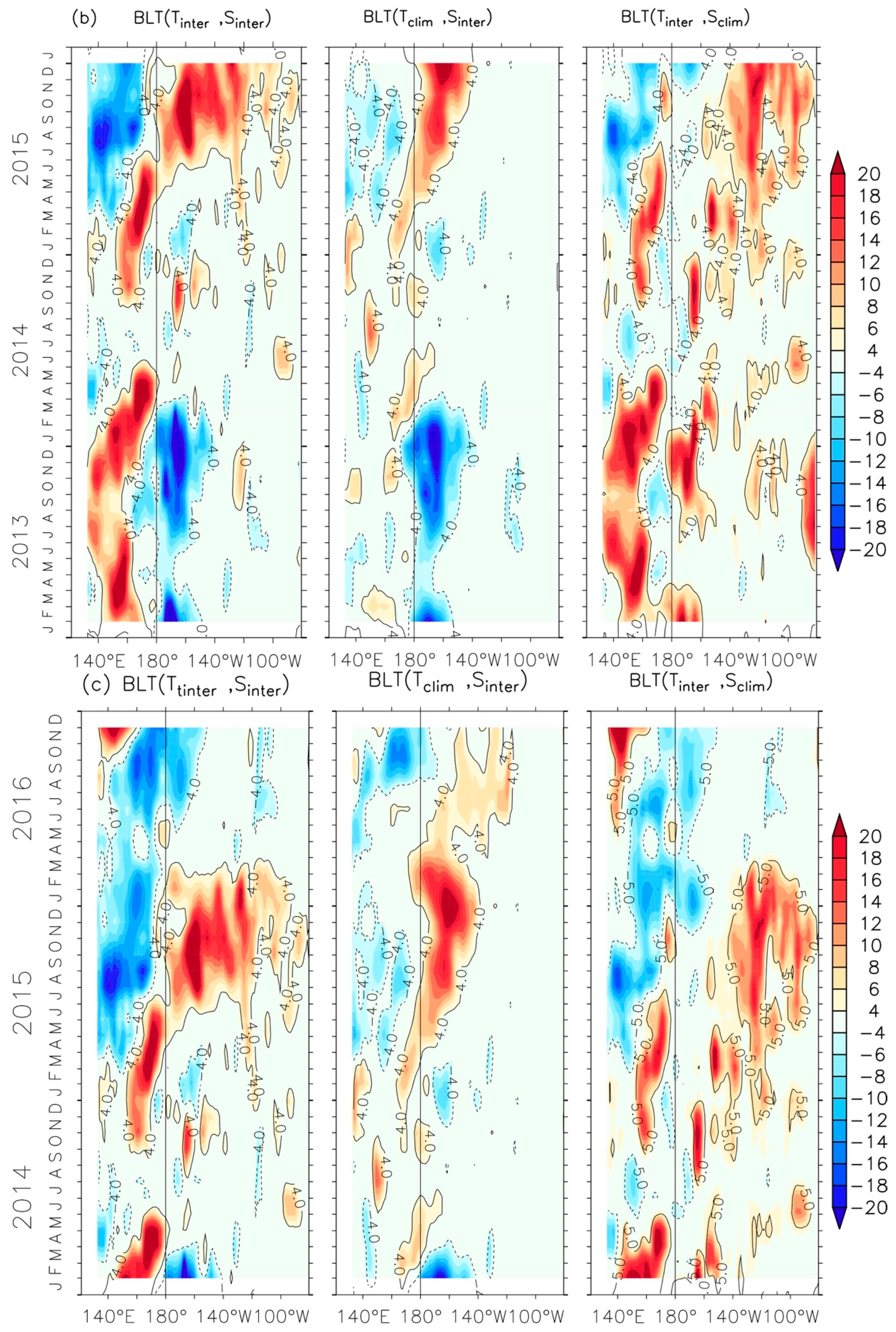
In order to explore the relationship between the SSSA and the SSTA during the three ENs, the BLT anomaly was examined in detail. It was found that during the three ENs, a negative BLT anomaly appeared as early as November of the early winter in the tropical Pacific (150° E–170° E) (
Figure 4). As seen from the characteristics of the BL distribution corresponding to the SSSA during the three ENs, it was demonstrated that the positive BLT anomaly in the western Pacific coexisted with the positive SSTA in the central-eastern Pacific during the EN. Before the ENs, the BLT in the western equatorial Pacific was thicker than that in the central-eastern Pacific, with a relatively significant positive anomaly. Subsequently, the thick BLT moved from the west to the east of the dateline, resulting in an enhanced positive BLT anomaly, which was accompanied by the increase of a negative BLT anomaly in the western equatorial Pacific. At the peak of the EN in the winter of 1997, a large positive BLT anomaly appeared significantly to the east of the dateline in the western-central equatorial Pacific. The region of the positive BLT anomaly spanned more than 40 longitudes, lasting from August 1997 until the boreal spring of 1998. Note that the positive BLT anomaly is consistent with the negative SSSA in 1997–1998 (
Figure 4a). By comparing the distribution of the BLT anomaly during the 2015/2016 EN with that during the 1997/1998 EN, it was found that the negative BLT anomalies in the western Pacific continued strengthening in the evolutions of the two extreme ENs with an eastward movement, enhancement, and expansion of the positive BLT anomaly near the dateline in the previous winter (
Figure 4c). The BL near the dateline significantly thickened and obviously corresponded to the negative SSSA. However, there was a difference in BL evolution between the two ENs at the peak of EN. For instance, the location of the positive BLT anomaly in 2015–2016 was more westward than that in 1997, which led to greater sea surface heat accumulation in the Niño 3.4 region in 2015. This partly explains why the Niño3.4 index of 2015/2016 EN was stronger than that of the 1997/1998 EN. For the 2014/2015 weak EN, the BL in the western Pacific becomes thin at the pre-period (from December 2013 to January 2014), leading to the positive anomaly with a peak (>12 m) west of the dateline, and a significant enhancing and eastward-extending trend (
Figure 4b). However, the positive BLT anomaly decreases and disappears rapidly in the early summer of 2014, with a weak negative SSSA during the 2014/2015 EN. The interruption of BL thickening in the central-western equatorial Pacific resulted in the maintenance of vertical heat transfer in this region and the unsustainable sea surface heat accumulation. This is one of the obvious reasons why the SSTA of this weak EN failed to develop during 2014/2015 EN.
5. Modulation of SSSA on BLT
BLT is mainly dominated by temperature and salinity. Zheng and Zhang [
49] have analyzed the relationships among BLT, temperature, and salinity during a La Niña event in detail. Additional research has demonstrated that although the effect of temperature on the stratification is decisive, the effect of salinity variation on the density of the mixed layer and stratification is greater than that of temperature in the WP (2° S–2° N, 160°–180° E) of the equatorial Pacific. Salinity affects the decisive factors of the vertical entrainment process in the equatorial Pacific [
23,
41,
49,
50,
51]. The salinity field in the tropical Pacific near the dateline regulates the MLD by changing the seawater density, which indirectly affects the interannual variation of the BLT. In the WP of the western Pacific, the BL limits the vertical heat exchange by ocean stratification, leading to surface heat accumulation, and ultimately generating positive feedback on SST.
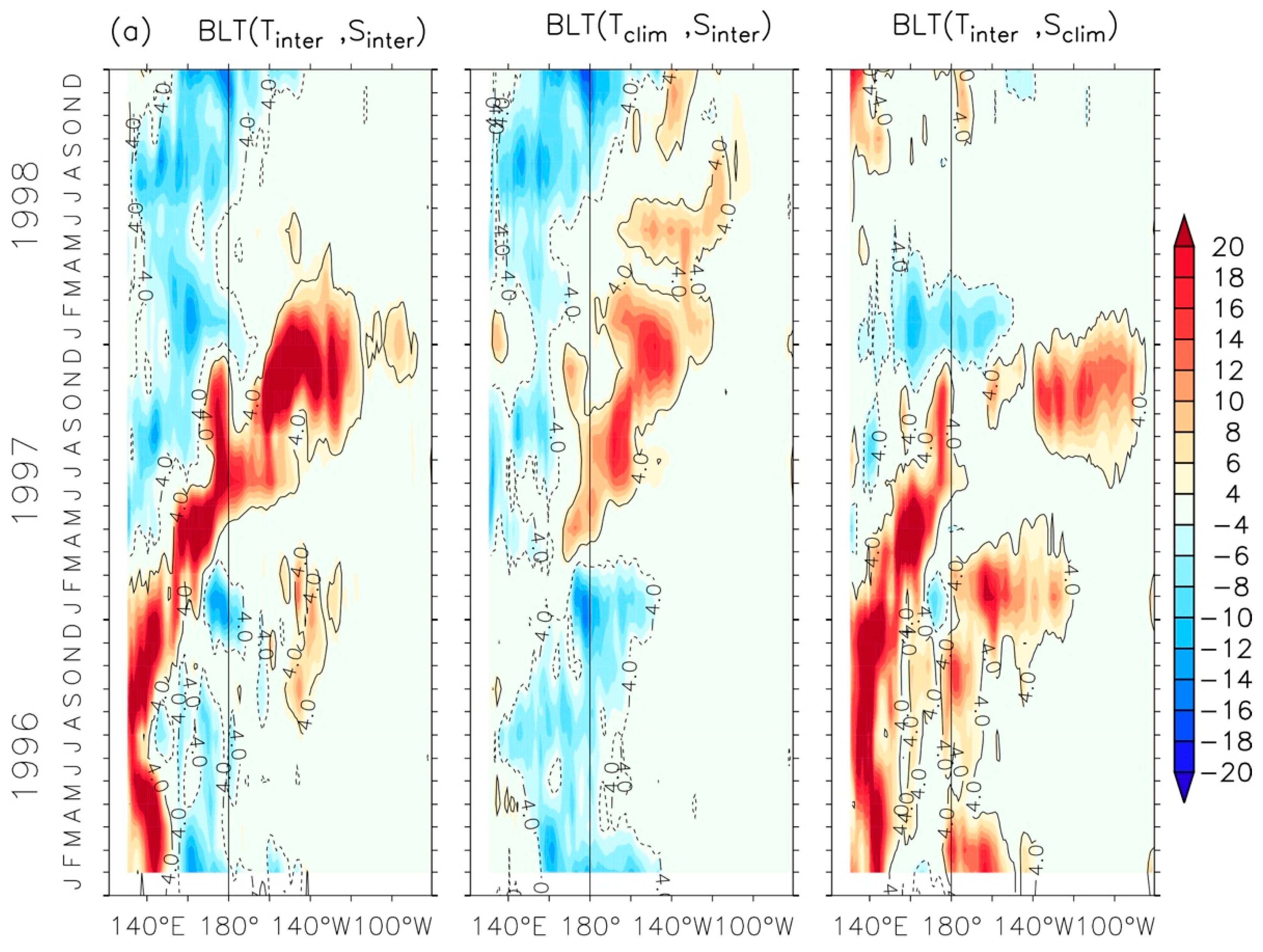
For the three ENs, the characteristics of the BLT spatial-temporal variation show a relatively clear correspondence to the SSSAs. In order to distinguish the relative contributions of salinity and temperature variations on the BLT anomaly during ENs, the method derived from Zheng and Zhang [
50] was used (
Table 1), in which it is assumed that BLT is only a function of T and S. BLT (
Tinter,
Sinter) represents a referenced interannual variation analysis of BLT, including
Tinter and
Sinter (the interannual variability of temperature and salinity). BLT (
Tinter,
Sclim) is the analysis of temperature and salinity interannual variation in climatology. BLT (
Tclim,
Sinter) is the analysis of temperature in climatology and interannual variation of salinity. BLT (
Tclim,
Sclim) is the analysis of salinity and temperature in climatology. The purpose of these comparisons was to verify the sensitivity of BLT anomalies to interannual variations of temperature and salinity during ENs.
Figure 5 shows the evolutions of BLT over the ENSO cycle under different influential factors during the three ENs. From the distribution of BLT (
Tinter,
Sinter) during three ENs, it can be seen that obvious positive BLT anomalies appear in the tropical western-central Pacific from the winter of the EN year until the following spring, as has been discussed in detail in the above section. By comparing the contributions of the interannual variations of T and S to the BLT anomaly in the 1997/1998 EN, it was found that the BLT corresponding to interannual variations of salinity present a positive BLT anomaly in the same region as observed. The BLT with tinter does not show the positive BLT anomaly in the corresponding region (
Figure 5a). During other ENs, the BLT is sensitive to sinter as well, and similar positive BLT anomalies show up in the tropical western-central Pacific (
Figure 5b,c). For the two strong ENs, only when the influence of salinity variations is considered, does the BLT begin to show obvious positive anomalies east of the dateline from June of the EN year, and they are generally maintained until the following spring. However, in the summer of 2014, there is no obvious positive anomaly near the dateline, indicating that the effect of interannual variation in salinity is weak. The similarity of the three ENs is such that, in June of the EN year, the BL begins to significantly thicken under the influence of the salinity interannual anomaly in the area of 180°–140° W in the equatorial Pacific, in which the regional BLT anomaly plays a primary role in the development and maturity of ENs.
Based on the characteristics of BLT variation during the three ENs, it was found that in EN evolution, the SSSA is a main factor for regulating BLT variability. Even the weak SSSA during the 2014/2015 EN showed the same corresponding relationship, and the relationship between the BLT anomaly in the key region and the SSSA during the EN was further verified. Therefore, it is believed that the weak variability of the BL caused by the weak salinity variation in the summer of 2014 due to small heat accumulation on the sea surface than other strong ENs.
6. SSS Tendency and its Possible Forcing Factors
To clarify the possible forcing factors on the salinity budget, the balance equation related to salinity is presented. This approach has been widely used to study the mixed layer salinity tendency in ocean conditions and processes [
36,
38,
52,
53,
54,
55]. In particular, if the study region is over the tropical Pacific and the salinity budget is ignored, the eddy-scale mixing processes, are governed by the simplified equation as follows.
where
is the tendency of the mixing layer salinity; and
A,
D and
F on the right side of equation represent the tendency affected by the surface advection, subsurface forcing, and surface forcing, respectively, as defined by Zhang et al. [
36] and Zhi et al. [
38] in detail. Changes in FWF, advection, and horizontal and vertical diffusion that could affect SSS variations in the tropical Pacific at the interannual scale were examined.
6.1. SSS Tendency and its Budget
As seen in
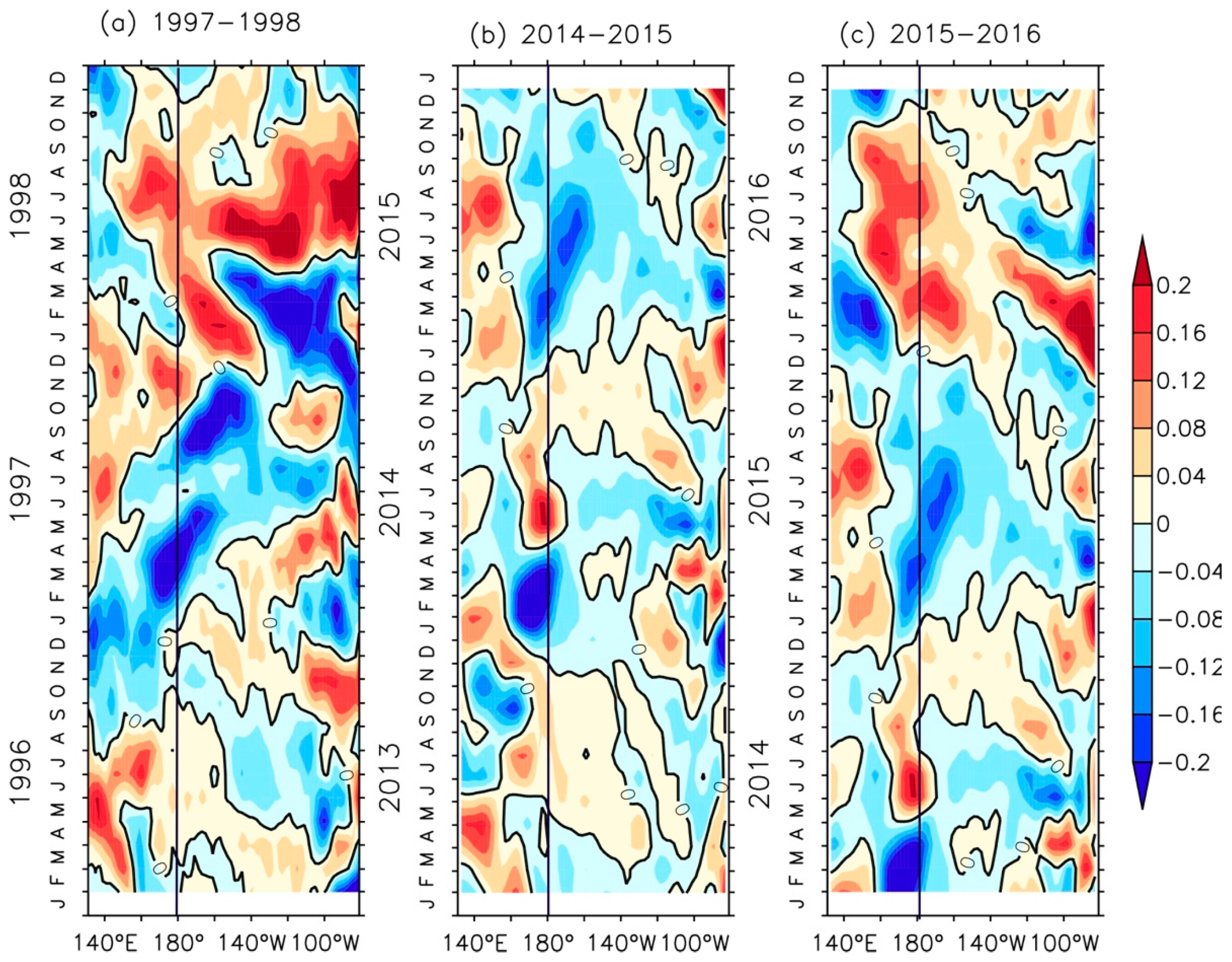
Figure 6, the SSS tendency west of the dateline shows a significant negative value during the spring of all three ENs, indicating that SSS has a significant decreasing trend. In addition, the appearance of a significant negative SSS tendency leads the variations of SSSA and SSTA by three months or more. The large negative SSS tendency appearing during every EN lasts for a long time, leading to a negative SSSA until the EN weakens. For example, in the early spring of both 1998 and 2016, when the SSS tendency rapidly switches from negative to positive, the SSTA begins to weaken rapidly in the same period or 1–2 months later, exhibiting the termination signal of EN. During the 2014/2015 EN, the salinity tendency shifts from negative to positive in August 2014. Therefore, whether the salinity tendency in the region east of the dateline has a shift between positive and negative, and whether salinity increases or the decreases in the first half of the EN year may serve as indicators for predicting whether EN will continue to develop.
Based on the above analyses, it was illustrated that the SSSA and its tendency were not synchronous during the three ENs, resulting in a significant difference in the feedback on SST. The induction shows that the SSSA and tendency appear as a negative anomaly in the early EN period and those that are sufficiently strong are necessary and sufficient conditions. For example, near the dateline in January 1997, the SSS decreases rapidly, while the obvious negative tendency moves slowly to the east of the dateline (
Figure 6a). In contrast, the negative tendency near the dateline in January of 2015 is relatively weak (<0.1 psu/month) and lasts for nearly eight months (
Figure 6c), longer than that in 1997. In addition, salinity decreases continuously, and the increasing magnitude of the negative tendency is clearly large in the equatorial eastern-central Pacific (170° E–150° W) throughout 2015. The positive salinity tendency appears in the early spring of 2016, when the EN decays from the perspective of the SSTA evolution (
Figure 1c). Salinity tendency near the dateline suddenly changes from negative to positive in May of 2015 (
Figure 6b) and then the positive tendency increases in 170° E–150° W in June, which shows a significant difference in evolution compared with strong events. In this process, the negative salinity tendency lasts for a short time, and disappears from April to May in the early summer of the EN, with the increasing salinity anomaly. In June and July of 2014, the positive salinity tendency rapidly increases to 0.2 psu/month, which only appears in the later period of strong ENs. The shift of this salinity tendency from negative to positive also foreshadows the termination of warming during the 2014/2015 EN. What causes the rapid weakening of SSS near the dateline during the three ENs, and what causes the sudden significant positive change of SSS in the summer of 2014, suppressing the evolution of this EN?
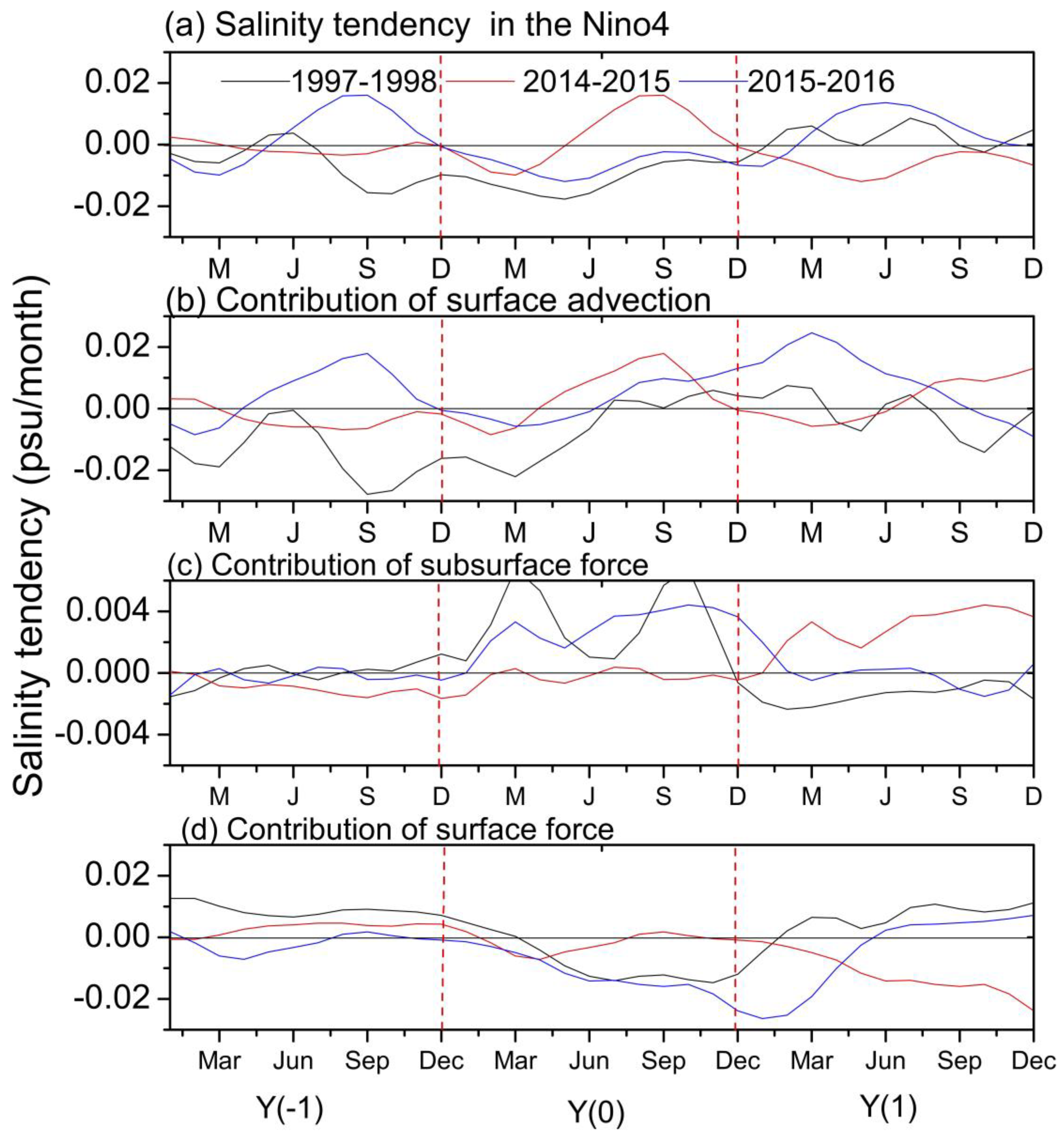
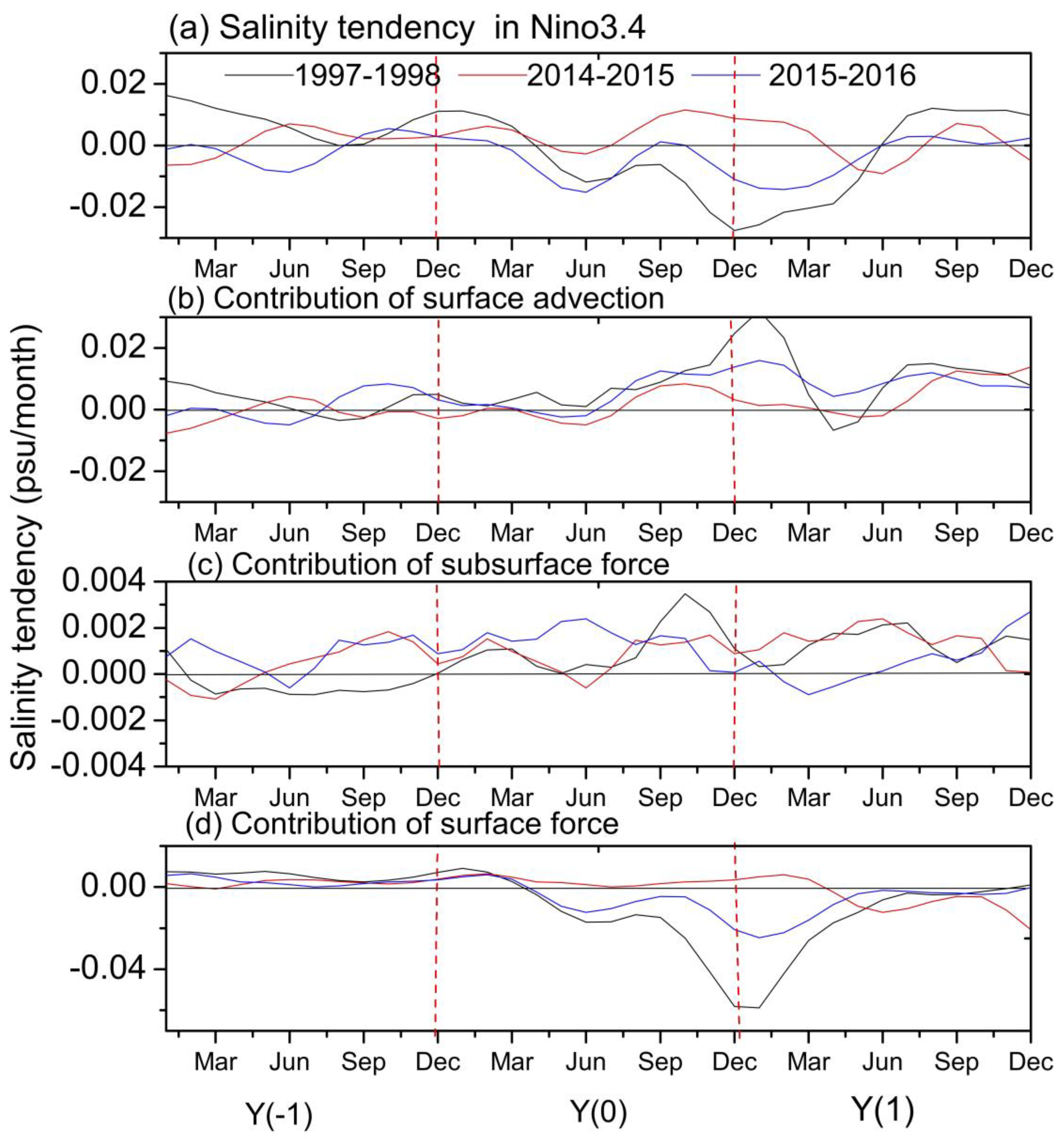
Next, causes for the SSS variability were analyzed during each EN. Budget terms affecting the tropical SSS balance include surface advection, and subsurface and surface forcing, defined as the salinity budget equation. The evolution of the average salinity tendency in two Niño regions during the three ENs is given to compare the contributions of factors to the tendency (
Figure 7 and
Figure 8). As can be seen, the evolutions of surface advection and the salinity tendency in the western tropical Pacific (Niño 4 region) before ENs are quite similar, indicating its prominent role in this period. This means that the surface forcing also certainly affects its negative anomaly, but the subsurface forcing is not significant before ENs. Therefore, salinity anomalies are mainly affected by the horizontal advection and surface forcing [
53,
55].
With the evolution of EN, the negative surface forcing has gradually increased since the spring of the EN year, which plays an important role in decreasing SSS in the equatorial Pacific. In the early period of EN evolution, the contributions of surface advection and surface forcing offset the effect of subsurface forcing. However, the effect of surface advection decreases rapidly after June, so that the surface forcing becomes the main contributor to the reduction of salinity, causing the negative salinity tendency in Niño 4 from the EN summer to the following spring. In addition, during the 2014/2015 EN, the dominant term of salinity variation is the horizontal advection after May of 2015, which brings high salinity water, prompting the increase of salinity near the dateline in the summer of 2014. It is worth noting that, in an obvious difference from the processes of the two strong ENs, the reducing-salinity effect of surface forcing does not increase gradually, leading to a sudden positive salinity change on the dateline in the key region. If the more apparent entrainment process in the western equatorial Pacific is ignored (
Figure 8), the effect of surface forcing will be more apparent, while the surface advection during the three ENs is weak. During the strong ENs, the effect of surface forcing begins to appear from the spring of the EN year, and the rapid increase shows in March of 1997 and 2016. The negative tendency of salinity is mostly determined by the surface forcing in these two processes. However, in the weak process, the weak surface forcing slightly affects the negative salinity variation in the spring of 2014, leading to the smooth evolution of the SSSA. Therefore, in the summer of 2014, under the positive effects of other factors, the salinity does not decrease, but continues to increase. The reason why this EN process does not continue to develop in 2014 may be related to the obvious FWF abnormality, which is analyzed in the following section.
6.2. Causes of SSSA during ENSO
The above section showed that the surface forcing related to FWF plays a prominent role in the surface salinity tendency in the tropical Pacific during ENs. Moreover, the evolution of a spatial and temporal FWF anomaly in the three ENs (
Figure 9) is highly consistent with that of the SSSA (
Figure 2). The negative FWF anomaly appears in the western edge of the WP between 150° E and 165° E in March of the EN year during the three ENs. However, the negative FWF anomaly in 2014 is inconsistent with the strengthening and eastward-moving FWF in the summer of the EN; furthermore, the negative FWF anomaly in 2014 begins to weaken and fade until December of 2014, consistent with the negative tendency of displacement and the negative SSSA during the 2014/2015 EN. However, in the spring of 2014 the weak negative FWF anomaly in the eastern-central Pacific slows down the negative SSS tendency. In contrast, corresponding to the clear appearance of the negative SSS tendency in 1997 and 2015, the negative FWF anomaly appears near the dateline in the spring of the EN year, leading to a strong SSS anomaly by two months. It is worth noting that in the spring of 1997, the salinity tendency shifts to negative before the negative FWF anomaly, which may be related to the significant horizontal advection in 1997 (
Figure 7), and it has an impact on the salinity change, together with FWF.
It was inferred that during ENs, the FWF anomaly leads to the SSSA in the WP, pushing the warm/fresh water mass to the east. This then meets the westward high salinity water near the dateline, forming a salt front with strong salinity gradient, and affecting the upper-ocean vertical stratification. For instance, in the early stage of ENs, the negative FWF anomaly in the key region leads to the rapid decrease of salinity in the high-salinity area. This leads to the decrease in the sea surface density, thus inducing a thickening in the BLT through affecting the vertical movement and mixing of seawater. Consequently, the thickening in the BLT reduces the vertical heat transfer and increases heat accumulation in the upper layer, which finally affects the SSTA development. In the early EN, precipitation, as a direct source of FWF, has a direct effect on the SSS tendency.
7. Discussion and Conclusions
The 2015/2016 EN is regarded as an extreme event after the super strong ENs of 1982/1983 and 1997/1998 and has been identified as the event with the strongest peak intensity since 1950 [
7]. We have analyzed the processes underlying the onset and evolution of recent ENs from a new perspective, i.e., the relationship between the ENSO and the interannual SSS anomaly in the tropical Pacific, which advances our understanding of ENSO.
By comparing three ENs, we have further verified the relationships among ENSO, SSS changes in the equatorial Pacific, and salinity-related physics during strong ENs. The evolution of salinity during the three ENs indicated that the SSS is consistent with the evolution of the ENSO. During the 1997/1998 and 2015/2016 ENs, there were significant positive SSS anomalies located west of the dateline. With the evolution of the EN, the SSS caused by the ENSO decreased in the western equatorial Pacific, forming sharp salinity gradients, and the maximum SSSA lasted from summer to winter in EN years. However, during the 2014/2015 EN, the negative SSSA in the western equatorial Pacific was not obvious and disappeared after the appearance of a positive anomaly near the dateline. However, the SSSA in 2015 was re-stimulated and developed for about three months before the occurrence of the SSTA. We have analyzed the processes through which salinity affects EN by influencing the BLT and SST, and the possible signal of the termination of EN during the three ENs.
Surface forcing is a major factor affecting the salinity budget. The early FWF anomaly in the western tropical Pacific had the most significant impact, leading to the decisive role of surface forcing on the salinity change. Compared with the two strong ENSO events, the corresponding early FWF anomaly did not propagate eastward in 2014–2015, and the FWF negative anomaly weakened, inhibiting the early warming of the eastern Pacific Ocean. The early SSS in the central and western Pacific may serve as the index of SSTA for salinity change, which is closely linked to the ENSO. In particular, the salinity anomaly not only affects the strength of SSTA in the ocean, it can also act as a precursor for the ENSO evolution and intensity.
Both salinity and its relevant physical processes are important for the evolution of a successful EN, while the lack of such processes may lead to the failure of an ENSO event [
56]. The differences between the three ENs were mainly considered, and the potential impact of the salinity mechanism during the 2014/2015 EN on the onset and evolution of the later 2015/2016 EN needs qualitative research. In the analysis of the salinity impact on ENSO in this paper, only the equatorial Pacific region was considered, with insufficient attention to other regions. Other significant areas will be studied to obtain their internal mechanisms. There may be some uncertainties in the conclusions. The extreme, strong EN cases are limited and couple model simulation may provide additional strong EN cases. However, the coupling models have some biases in simulating ENSO (including their amplitudes and position, the central Pacific and eastern Pacific ENSO) and salinity cause-effect, because of the existence of the double Intertropical Convergence Zone (ITCZ). Thus, the salinity contribution to ENSO (different types) in the coupled models needs to be evaluated.
More importantly, salinity anomaly is not only an early signal for the SSTA in the key region but is also a possible dynamic factor for generating a strong EN through an early salinity anomaly. Based on two extreme ENs and one weak EN, the comparison presented certain distinct features, and both the evolution and the related physics in strong ENs were different from the weak EN. However, there has been no systematic study on the significant effects of salinity on general ENs. We could further compare the classic ENs by analyzing the role of salinity, as in this paper. In addition, the complexity of the ENSO also needs to be analyzed by combining the global warming and decadal change, since some have argued that recent ENSO events are closely related to global warming. Future studies may lead to more advancements when placing salinity variation in the context of climate change.


