Evidence for Rayleigh-Taylor Plasma Instability at the Front of Solar Coronal Mass Ejections


Abstract
:1. Introduction
2. Observations
3. Analysis and Results
3.1. Wavelet Amplitude Spectrum
3.2. Amplitude Hovmöller
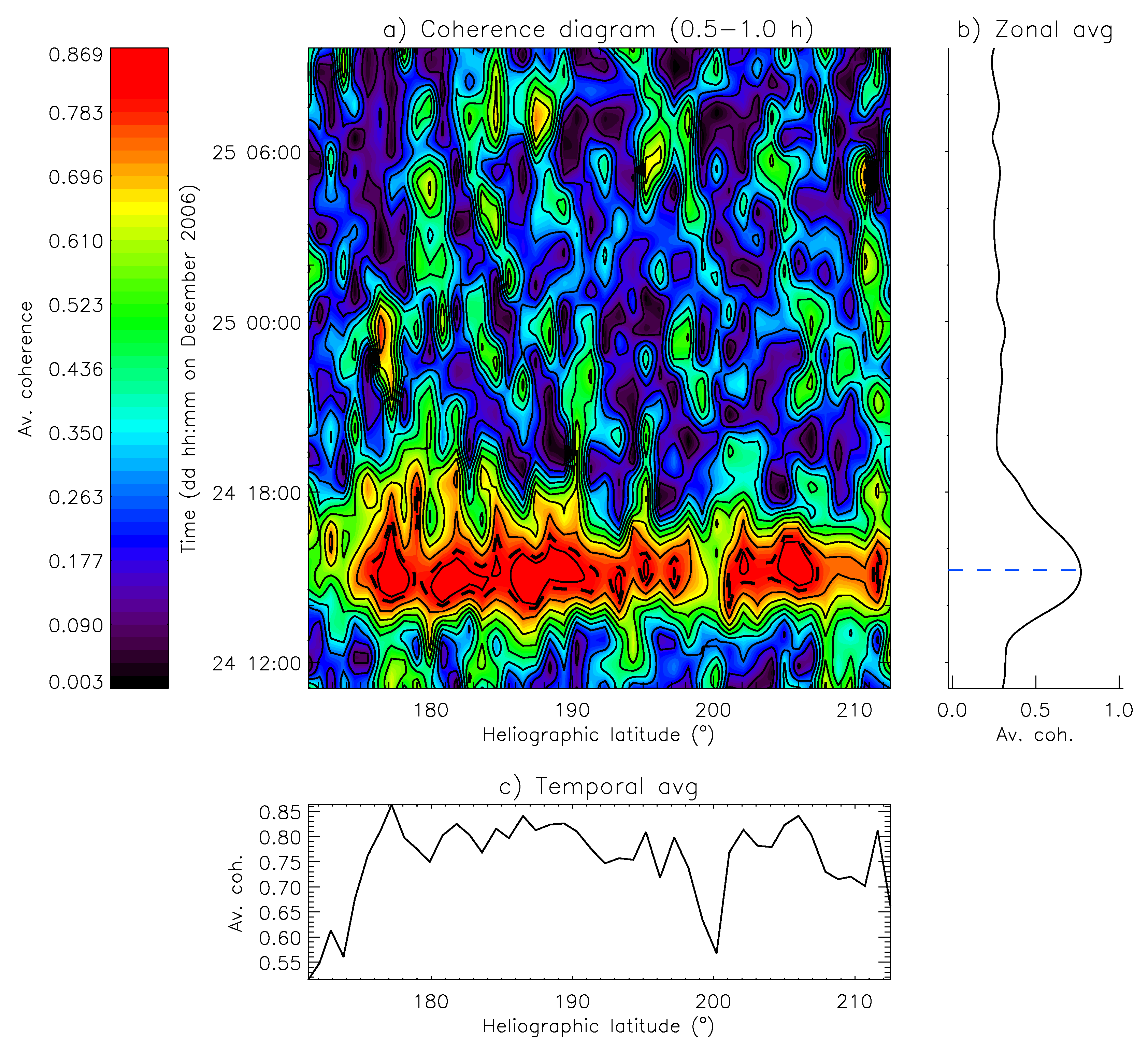
3.3. Wavelet Coherence
4. Discussion
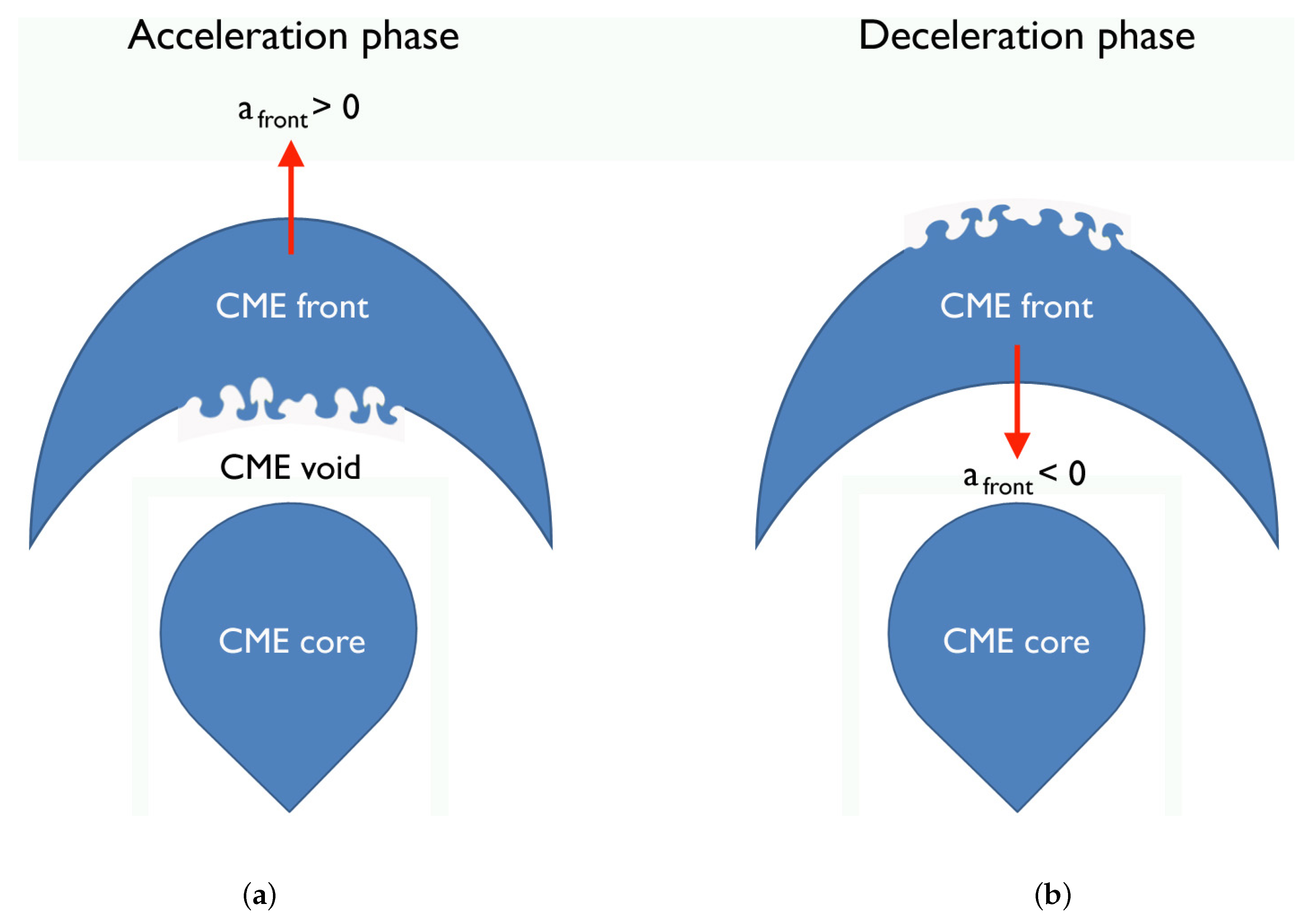
5. Interpretation
6. Conclusions
Author Contributions
Funding
Conflicts of Interest
References
- Webb, D.F. Coronal mass ejections: The key to major interplanetary and geomagnetic disturbances. Rev. Geophys. 1995, 33, 577–583. [Google Scholar] [CrossRef]
- Sheeley, N.R., Jr.; Walters, J.H.; Wang, Y.M.; Howard, R.A. Continuous tracking of coronal outflows: Two kinds of coronal mass ejections. J. Geophys. Res. Space Phys. 1999, 104, 24739–24767. [Google Scholar] [CrossRef]
- Aschwanden, M.J.; Caspi, A.; Cohen, C.M.S.; Holman, G.; Jing, J.; Kretzschmar, M.; Kontar, E.P.; McTiernan, J.M.; Mewaldt, R.A.; O’Flannagain, A.; et al. Global Energetics of Solar Flares. V. Energy Closure in Flares and Coronal Mass Ejections. Astrophys. J. 2017, 836, 17. [Google Scholar] [CrossRef] [Green Version]
- Raymond, J.C.; Thompson, B.J.; St. Cyr, O.C.; Gopalswamy, N.; Kahler, S.; Kaiser, M.; Lara, A.; Ciaravella, A.; Romoli, M.; O’Neal, R. SOHO and radio observations of a CME shock wave. Geophys. Res. Lett. 2000, 27, 1439–1442. [Google Scholar] [CrossRef]
- Mancuso, S.; Raymond, J.C.; Kohl, J.; Ko, Y.-K.; Uzzo, M.; Wu, R. UVCS/SOHO observations of a CME-driven shock: Consequences on ion heating mechanisms behind a coronal shock. A&A 2002, 383, 267–274. [Google Scholar] [CrossRef] [Green Version]
- Korreck, K.E.; Zurbuchen, T.H.; Lepri, S.T.; Raines, J.M. Heating of Heavy Ions by Interplanetary Coronal Mass Ejection Driven Collisionless Shocks. Astrophys. J. 2007, 659, 773–779. [Google Scholar] [CrossRef] [Green Version]
- Reames, D.V. Particle acceleration at the Sun and in the heliosphere. Space Sci. Rev. 1999, 90. [Google Scholar] [CrossRef]
- Chrysaphi, N.; Kontar, E.P.; Holman, G.D.; Temmer, M. CME-driven Shock and Type II Solar Radio Burst Band Splitting. Astrophys. J. 2018, 868, 79. [Google Scholar] [CrossRef] [Green Version]
- Zucca, P.; Morosan, D.E.; Rouillard, A.P.; Fallows, R.; Gallagher, P.T.; Magdalenic, J.; Klein, K.-L.; Mann, G.; Vocks, C.; Carley, E.P.; et al. Shock location and CME 3D reconstruction of a solar type II radio burst with LOFAR. A&A 2018, 615, A89. [Google Scholar] [CrossRef] [Green Version]
- Attrill, G.D.R.; Harra, L.K.; van Driel-Gesztelyi, L.; Démoulin, P. Coronal “Wave”: Magnetic Footprint of a Coronal Mass Ejection? Astrophys. J. 2007, 656, L101–L104. [Google Scholar] [CrossRef]
- Van Driel-Gesztelyi, P.; Démoulin, J.L.; Culhane, S.A.; Matthews, L.K.; Harra, C.H.; Mandrini, K.L.; Klein, H.; Kurokawa, C.P.G.L. A Multiple Flare Scenario where the Classic Long-Duration Flare Was Not the Source of a CME. Sol. Phys. 2007, 240. [Google Scholar] [CrossRef]
- Bemporad, A.; Soenen, A.; Jacobs, C.; Landini, F.; Poedts, S. SIDE Magnetic Reconnections Induced by Coronal Mass Ejections: Observations and Simulations. Astrophys. J. 2010, 718, 251–265. [Google Scholar] [CrossRef]
- Low, B.C. Coronal mass ejections, magnetic flux ropes, and solar magnetism. J. Geophys. Res. Space Phys. 2001, 106, 25141–25163. [Google Scholar] [CrossRef]
- Foullon, C.; Verwichte, E.; Nakariakov, V.M.; Nykyri, K.; Farrugia, C.J. Magnetic kelvin-helmholtz instability at the sun. Astrophys. J. 2011, 729, L8. [Google Scholar] [CrossRef]
- Ofman, L.; Thompson, B.J. Sdo/aia observation of kelvin–helmholtz instability in the solar corona. Astrophys. J. 2011, 734, L11. [Google Scholar] [CrossRef]
- Domingo, V.; Fleck, B.; Poland, A.I. The SOHO Mission, 1st ed.; Springer: Dordrecht, The Netherlands, 1996. [Google Scholar] [CrossRef]
- Brueckner, G.E.; Howard, R.A.; Koomen, M.J.; Korendyke, C.M.; Michels, D.J.; Moses, J.D.; Socker, D.G.; Dere, K.P.; Lamy, P.L.; Llebaria, A.; et al. The Large Angle Spectroscopic Coronagraph (LASCO). Sol. Phys. 1995, 162. [Google Scholar] [CrossRef]
- De Moortel, I.; Ireland, J.; Walsh, R. Observation of oscillations in coronal loops. A&A 2000, 355, L23–L26. [Google Scholar]
- Morgan, H.; Habbal, S.R.; Li, X. Hydrogen Lyα Intensity Oscillations Observed by theSolar and Heliospheric ObservatoryUltraviolet Coronagraph Spectrometer. Astrophys. J. 2004, 605, 521–527. [Google Scholar] [CrossRef]
- Bloomfield, D.S.; McAteer, R.T.J.; Lites, B.W.; Judge, P.G.; Mathioudakis, M.; Keenan, F.P. Wavelet Phase Coherence Analysis: Application to a Quiet-Sun Magnetic Element. Astrophys. J. 2004, 617, 623–632. [Google Scholar] [CrossRef]
- Telloni, D.; Bruno, R.; D’Amicis, R.; Pietropaolo, E.; Carbone, V. Wavelet analysis as a tool to localize magnetic and cross-helicity events in the solar wind. Astrophys. J. 2012, 751, 19. [Google Scholar] [CrossRef]
- Telloni, D.; Perri, S.; Bruno, R.; Carbone, V.; Amicis, R.D. An analysis of magnetohydrodynamic invariants of magnetic fluctuations within interplanetary flux ropes. Astrophys. J. 2013, 776, 3. [Google Scholar] [CrossRef]
- Bemporad, A.; Matthaeus, W.H.; Poletto, G. Low-Frequency Lyα Power Spectra Observed by UVCS in a Polar Coronal Hole. Astrophys. J. 2008, 677, L137–L140. [Google Scholar] [CrossRef]
- Telloni, D.; Bruno, R.; Carbone, V.; Antonucci, E.; D’Amicis, R. Statistics of density fluctuations during the transition from the outer solar corona to the interplanetary space. Astrophys. J. 2009, 706, 238–243. [Google Scholar] [CrossRef]
- Dolla, L.; Marqué, C.; Seaton, D.B.; Doorsselaere, T.V.; Dominique, M.; Berghmans, D.; Cabanas, C.; Groof, A.D.; Schmutz, W.; Verdini, A.; et al. Time delays in quasi-periodic pulsations observed during the x2.2 solar flare on 2011 february 15. Astrophys. J. 2012, 749, L16. [Google Scholar] [CrossRef]
- Torrence, C.; Compo, G.P. A Practical Guide to Wavelet Analysis. Bull. Am. Meteorol. Soc. 1998, 79, 61–78. [Google Scholar] [CrossRef] [Green Version]
- Percival, D.P. On estimation of the wavelet variance. Biometrika 1995, 82, 619–631. [Google Scholar] [CrossRef]
- Spiegel, M.R. Schaum’s Outline of Theory and Problems of Probability and Statistics; Mcgraw-Hill: New York, NY, USA, 1975. [Google Scholar]
- Telloni, D.; Antonucci, E.; Bruno, R.; D’Amicis, R. Persistent and self-similar large-scale density fluctuations in the solar corona. Astrophys. J. 2009, 693, 1022–1028. [Google Scholar] [CrossRef]
- Arons, J.; Lea, S.M. Accretion onto magnetized neutron stars - Structure and interchange instability of a model magnetosphere. Astrophys. J. 1976, 207, 914. [Google Scholar] [CrossRef]
- Robinson, K.; Dursi, L.J.; Ricker, P.M.; Rosner, R.; Calder, A.C.; Zingale, M.; Truran, J.W.; Linde, T.; Caceres, A.; Fryxell, B.; et al. Morphology of Rising Hydrodynamic and Magnetohydrodynamic Bubbles from Numerical Simulations. Astrophys. J. 2004, 601, 621–643. [Google Scholar] [CrossRef] [Green Version]
- Hester, J.J.; Stone, J.M.; Scowen, P.A.; Jun, B.I.; John, S.I.G.; Norman, M.L.; Ballester, G.E.; Burrows, C.J.; Casertano, S.; Clarke, J.T.; et al. WFPC2 Studies of the Crab Nebula. III. Magnetic Rayleigh-Taylor Instabilities and the Origin of the Filaments. Astrophys. J. 1996, 456, 225. [Google Scholar] [CrossRef] [Green Version]
- Isobe, H.; Miyagoshi, T.; Shibata, K.; Yokoyama, T. Three-Dimensional Simulation of Solar Emerging Flux Using the Earth Simulator I. Magnetic Rayleigh-Taylor Instability at the Top of the Emerging Flux as the Origin of Filamentary Structure. Publ. Astron. Soc. Jpn. 2006, 58, 423–438. [Google Scholar] [CrossRef] [Green Version]
- Berger, T.E.; Slater, G.; Hurlburt, N.; Shine, R.; Tarbell, T.; Title, A.; Lites, B.W.; Okamoto, T.J.; Ichimoto, K.; Katsukawa, Y.; et al. Quiescent prominence dynamics observed with thehinodesolar optical telescope. i. turbulent upflow plumes. Astrophys. J. 2010, 716, 1288–1307. [Google Scholar] [CrossRef]
- Innes, D.E.; Cameron, R.H.; Fletcher, L.; Inhester, B.; Solanki, S.K. Break up of returning plasma after the 7 June 2011 filament eruption by Rayleigh-Taylor instabilities. A&A 2012, 540, L10. [Google Scholar] [CrossRef] [Green Version]
- Carlyle, J.; Williams, D.R.; van Driel-Gesztelyi, L.; Innes, D.; Hillier, A.; Matthews, S. Investigating the dynamics and density evolution of returning plasma blobs from the 2011 june 7 eruption. Astrophys. J. 2014, 782, 87. [Google Scholar] [CrossRef]
- Zhang, J.; Dere, K.P.; Howard, R.A.; Kundu, M.R.; White, S.M. On the Temporal Relationship between Coronal Mass Ejections and Flares. Astrophys. J. 2001, 559, 452–462. [Google Scholar] [CrossRef]
- Zhang, J.; Dere, K.P.; Howard, R.A.; Vourlidas, A. A Study of the Kinematic Evolution of Coronal Mass Ejections. Astrophys. J. 2004, 604, 420–432. [Google Scholar] [CrossRef] [Green Version]
- Qiu, J.; Wang, H.; Cheng, C.Z.; Gary, D.E. Magnetic Reconnection and Mass Acceleration in Flare–Coronal Mass Ejection Events. Astrophys. J. 2004, 604, 900–905. [Google Scholar] [CrossRef]
- Temmer, M.; Veronig, A.M.; Vršnak, B.; Rybák, J.; Gömöry, P.; Stoiser, S.; Maričić, D. Acceleration in Fast Halo CMEs and Synchronized Flare HXR Bursts. Astrophys. J. 2008, 673, L95–L98. [Google Scholar] [CrossRef] [Green Version]
- Jiang, B.; Chen, Y.; Wang, J.; Su, Y.; Zhou, X.; Safi-Harb, S.; DeLaney, T. Cavity of molecular gas associated with supernova remnant 3C 397. Astrophys. J. 2010, 712, 1147–1156. [Google Scholar] [CrossRef]
- Maloney, S.A.; Gallagher, P.T. Solar wind drag and the kinematics of interplanetary coronal mass ejections. Astrophys. J. 2010, 724, L127–L132. [Google Scholar] [CrossRef]
- Chandrasekhar, S. Hydrodynamic and Hydromagnetic Stability; Oxford University Press: Oxford, UK, 1961. [Google Scholar]
- Allen, C. Astrophysical Quantities; Springer: New York, NY, USA, 1973. [Google Scholar]
- Withbroe, G.L.; Kohl, J.L.; Weiser, H.; Munro, R.H. Probing the solar wind acceleration region using spectroscopic techniques. Space Sci. Rev. 1982, 33. [Google Scholar] [CrossRef]
- Noci, G.; Kohl, J.L.; Withbroe, G.L. Solar wind diagnostics from Doppler-enhanced scattering. Astrophys. J. 1987, 315, 706. [Google Scholar] [CrossRef]
- Bastian, T.S.; Pick, M.; Kerdraon, A.; Maia, D.; Vourlidas, A. The Coronal Mass Ejection of 1998 April 20: Direct Imaging at Radio Wavelengths. Astrophys. J. 2001, 558, L65–L69. [Google Scholar] [CrossRef] [Green Version]
- Mancuso, S.; Raymond, J.C.; Kohl, J.; Ko, Y.-K.; Uzzo, M.; Wu, R. Plasma properties above coronal active regions inferred from SOHO/UVCS and radio spectrograph observations. A&A 2003, 400, 347–353. [Google Scholar] [CrossRef] [Green Version]
- Cho, K.S.; Lee, J.; Gary, D.E.; Moon, Y.J.; Park, Y.D. Magnetic Field Strength in the Solar Corona from Type II Band Splitting. Astrophys. J. 2007, 665, 799–804. [Google Scholar] [CrossRef] [Green Version]
- Jensen, E.A.; Russell, C.T. Faraday rotation observations of CMEs. Geophys. Res. Lett. 2008, 35. [Google Scholar] [CrossRef] [Green Version]
- Chen, Y.; Feng, S.W.; Li, B.; Song, H.Q.; Xia, L.D.; Kong, X.L.; Li, X. A coronal seismological study with streamer waves. Astrophys. J. 2011, 728, 147. [Google Scholar] [CrossRef]
- Gopalswamy, N.; Nitta, N.; Akiyama, S.; Mäkelä, P.; Yashiro, S. Coronal magnetic field measurement from euv images made by thesolar dynamics observatory. Astrophys. J. 2011, 744, 72. [Google Scholar] [CrossRef]
- Kwon, R.Y.; Ofman, L.; Olmedo, O.; Kramar, M.; Davila, J.M.; Thompson, B.J.; Cho, K.S. Stereoobservations of fast magnetosonic waves in the extended solar corona associated with eit/euv waves. Astrophys. J. 2013, 766, 55. [Google Scholar] [CrossRef]
- Hariharan, K.; Ramesh, R.K.C.W.T.J. Simultaneous Near-Sun Observations of a Moving Type IV Radio Burst and the Associated White-Light Coronal Mass Ejection. Sol. Phys. 2016, 291. [Google Scholar] [CrossRef]
- Patsourakos, S.; Georgoulis, M.K. Near-Sun and 1 AU magnetic field of coronal mass ejections: A parametric study. A&A 2016, 595, A121. [Google Scholar] [CrossRef]
- Kooi, J.E.; Fischer, P.D.; Buffo, J.J.; Spangler, S.R. VLA Measurements of Faraday Rotation through Coronal Mass Ejections. Sol. Phys. 2017, 292. [Google Scholar] [CrossRef]
- Matsumoto, Y.; Hoshino, M. Onset of turbulence induced by a Kelvin-Helmholtz vortex. Geophys. Res. Lett. 2004, 31. [Google Scholar] [CrossRef]
- Zhang, W.; MacFadyen, A.; Wang, P. Three-dimensional relativistic magnetohydrodynamic simulations of the kelvin-helmholtz instability: Magnetic field amplification by a turbulent dynamo. Astrophys. J. 2009, 692, L40–L44. [Google Scholar] [CrossRef]
- Murphy, N.A.; Raymond, J.C.; Korreck, K.E. Plasma heating during a coronal mass ejection observed by thesolar and heliospheric observatory. Astrophys. J. 2011, 735, 17. [Google Scholar] [CrossRef]
- Fermi, E.; von Neumann, J. Taylor Instability of Incompressible Liquids. Part 1. Taylor Instability of an Incompressible Liquid. Part 2. Taylor Instability at the Boundary of Two Incompressible Liquids; Technical Report; Los Alamos Scientific Lab.: Los Alamos, NM, USA, 1953. [Google Scholar] [CrossRef]
- Livescu, D. Compressibility effects on the Rayleigh–Taylor instability growth between immiscible fluids. Phys. Fluids 2004, 16, 118–127. [Google Scholar] [CrossRef]


© 2019 by the authors. Licensee MDPI, Basel, Switzerland. This article is an open access article distributed under the terms and conditions of the Creative Commons Attribution (CC BY) license (http://creativecommons.org/licenses/by/4.0/).
Share and Cite
Telloni, D.; Carbone, F.; Bemporad, A.; Antonucci, E. Evidence for Rayleigh-Taylor Plasma Instability at the Front of Solar Coronal Mass Ejections. Atmosphere 2019, 10, 468. https://doi.org/10.3390/atmos10080468
Telloni D, Carbone F, Bemporad A, Antonucci E. Evidence for Rayleigh-Taylor Plasma Instability at the Front of Solar Coronal Mass Ejections. Atmosphere. 2019; 10(8):468. https://doi.org/10.3390/atmos10080468
Chicago/Turabian StyleTelloni, Daniele, Francesco Carbone, Alessandro Bemporad, and Ester Antonucci. 2019. "Evidence for Rayleigh-Taylor Plasma Instability at the Front of Solar Coronal Mass Ejections" Atmosphere 10, no. 8: 468. https://doi.org/10.3390/atmos10080468
APA StyleTelloni, D., Carbone, F., Bemporad, A., & Antonucci, E. (2019). Evidence for Rayleigh-Taylor Plasma Instability at the Front of Solar Coronal Mass Ejections. Atmosphere, 10(8), 468. https://doi.org/10.3390/atmos10080468