Article

High Contribution of Biomass Combustion to PM2.5 in the City Centre of Naples (Italy)

1
Department of Mathematics and Physics, Centre for Isotope Research on Cultural and Environmental heritage (CIRCE), Università degli Studi della Campania Luigi Vanvitelli, 81100 Caserta, Italy
2
Department of Science and Technology, Parthenope University of Naples, 80143 Napoli, Italy
3
Centre for Isotope Research (CIO) Energy and Sustainability Research Institute Groningen (ESRIG), University of Groningen, 9747 AG Groningen, The Netherlands
*
Author to whom correspondence should be addressed.
Atmosphere 2019, 10(8), 451; https://doi.org/10.3390/atmos10080451
Submission received: 23 July 2019 / Revised: 3 August 2019 / Accepted: 4 August 2019 / Published: 6 August 2019

Abstract

:
A better knowledge of the local and regional sources of the atmospheric particulate matter provides policy makers with the proper awareness when acting to improve air quality, in order to protect public health. A source apportionment study of the carbonaceous aerosol in Naples (Italy) is presented here, in order to improve this understanding in a vulnerable urban area. The aim of this study is quantifying directly fossil and non-fossil contributions to carbonaceous aerosol, by means of radiocarbon measurements. This is the first time that such an approach is implemented in this area. Fine particles with diameter ≤ 2.5 µm (PM2.5) were collected daily on top of a building in the city center, from November 2016 until January 2017. The carbonaceous aerosol was separated into organic carbon (OC) and elemental carbon (EC), by a two-step thermal desorption method. Subsequent radiocarbon analysis enabled the partitioning of the major sources of carbonaceous aerosol into fossil and non-fossil ones by applying radiocarbon isotopic mass balance. The PM2.5 concentration was on average 29 ± 3 µg⁄m3 (mean ± standard error; n = 18), with a maximum of 68.6 ± 0.7 µg⁄m3 on a day when air masses back-trajectories suggest a local origin and stagnant airflow conditions in the region. The carbonaceous component accounts for roughly half of the PM2.5 mass. Fossil fuel emissions are a minor source of OC (23%), but the dominant source of EC (66%), which is directly emitted during combustion processes. However, overall only 30% of the total carbon is of fossil origin, accounting for 14% of PM2.5 mass. Surprisingly, a comparable contribution is due to primary biomass burning carbon, which accounts in total for 15% of PM2.5 mass. Traffic pollution, the main cause of fossil fuel emissions in urban areas, is a significant, but not the predominant source of carbonaceous particle concentration. These findings support the conclusion of a predominant contribution from non-fossil sources to the carbon in airborne particulate matter, which policy makers should take into account when planning mitigation strategies to improve urban air quality.

1. Introduction

Since the beginning of the 1980s, the atmospheric science community has paid increasing attention to atmospheric aerosol particles, here addressed as particulate matter (PM), as shown by the rising number of publications on this subject [1]. PM is usually classified according to the size of the particles. Particles with a diameter less than or equal to 10 µm are classified as PM10. PM2.5 includes fine particles with a diameter less than or equal to 2.5 µm and it is a subset of PM10. The major chemical constituents of PM in the lower atmosphere are well known, but their relative contribution varies markedly with particle size range, geographic location and time of the year. Generally speaking, carbonaceous material, ammonium sulphate, ammonium nitrate, sodium nitrate, sea salts and other inorganic dusts are the most abundant constituents of PM [1,2,3,4]. Carbonaceous material, measured as total carbon (TC), forms a significant fraction of the aerosol mass, ranging from 21% to 56% at urban and background sites, in different European regions [5].
TC has traditionally been subdivided into organic carbon (OC) and elemental carbon (EC). OC includes all carbon bonded in the organic compounds present in the particle phase. EC is carbon, which is not bound to other elements. It is often seen as a proxy for black carbon, the most strongly light-absorbing fraction of aerosol carbon, even though strict definitions of both species are more complex than that and rely on properties of the particles and analytical methods [6]. EC is exclusively associated with primary emissions, because it is directly produced by combustion processes, whereas OC can be also formed through secondary pathways. Therefore, EC has been widely used as a tracer of the co-emitted primary OC [7,8,9]. Carbonaceous aerosol may also contain carbonate minerals, but mainly in the coarse fraction, i.e., the subset of PM10 not included in PM2.5 [4].
The attention paid to PM, in general, and to its carbonaceous fraction, in particular, has two reasons: the first is that aerosols of anthropogenic origin, especially fine particles, have a negative effect on public health [10,11]. The second reason is that they play a role in climate change, because they are responsible for radiative forcing of climate through both their direct interaction with radiation and as a result of their interaction with clouds [12]. The World Health Organization (WHO) guidelines report that PM2.5 should not exceed 10 μg/m3 annual mean, or 25 μg/m3 24-h mean [13]. A number of studies relate deleterious effects on human health directly to the carbonaceous fraction: this effect could be so pronounced that it is suggested that a reduction in ambient soot concentration (measured as EC concentration) would have a greater effect on health outcome than a reduction by the same fraction of PM2.5 or PM10 [1].
Due to the short lifetime (days to weeks) of tropospheric aerosol, concentrations tend to have strong regional and local signatures. In addition, aerosol characteristics and sources can differ among various sites, even when PM mass concentrations are similar. Therefore, abatement policies without detailed knowledge of PM constituents and their sources might be unnecessarily costly, inefficient and even counter-productive. A thorough understanding of the aerosol sources helps in designing a better legislation and reduction measures, aimed at limiting air pollution. However, too often PM10 and PM2.5 mass concentrations are the only aerosol metrics measured systematically in national and international air pollution monitoring networks [3].
The practice of source apportionment aims to break down the complexity of measured aerosol bulk into a finite number of particle components and it relates them to emission sources and/or production mechanisms. Source apportionment studies are usually based on approaches such as numerical analysis of correlations between various tracers and meteorological parameters or statistical evaluation of PM chemical data acquired at receptor sites. Model approaches are also used, ranging from chemical mass balance approaches to full dispersion models that simulate aerosol emissions, formation, transport and deposition [14].
Besides approaches applied to aerosol bulk mass, there are others based on analysis of specific PM fractions, such as isotopic mass balance of carbonaceous aerosols. This study belongs to the latter category.
Radiocarbon (14C) has proven the most powerful tracer to discriminate fossil fuel sources (e.g., vehicular exhaust and coal burning) from other sources with a recent signature (e.g., biomass burning and biogenic emissions) of carbonaceous aerosol [15,16,17,18,19,20,21,22,23,24]. In this case, a two-component model is used to quantify the contribution made by fossil fuel and non-fossil sources to TC or to its fractions, OC and EC, separately. This model merges together many actual sources into two end members (fossil fuel and non-fossil) based on their 14C isotopic signature and solves the isotopic balance analytically. 14C is a naturally occurring radioactive isotope with a half-life of 5730 years. It is constantly being produced in the lower stratosphere and upper troposphere by cosmic rays and removed by radioactive decay or by exchanges between the troposphere and the terrestrial biosphere or between the troposphere and the oceans. Therefore, a typical equilibrium concentration is established in the atmosphere. Living organisms assimilate 14C directly from atmospheric CO2 (autotrophic organisms) or indirectly through the trophic chain (heterotrophic organisms) and therefore have a 14C signature comparable to the contemporary atmosphere. Fossil sources are assumed to be 14C-free because their original 14C content decayed over time and they have not exchanged 14C with the atmosphere for millennia. During the last century, nuclear testing introduced a large amount of 14C in the atmosphere, changing abruptly the 14C atmospheric composition, until it was finally banned in 1963. Since then, this “bomb-spike” has been decreasing toward pre-bomb conditions, mainly due to the mixing and buffering effect of the ocean reservoirs of older C, but also due to dilution by the fossil emission related to human activities. Usually, in aerosol science, the 14C/12C ratio in a sample is compared to that in 1950 (modern, by definition). Aerosol carbon derived from presently living biomass, such as biogenic primary and secondary organic aerosols as well as aerosols from cooking emissions, have the 14C/12C ratio of the contemporary atmosphere. Plant materials, grown under higher level of bomb-spike condition, such as wood used for residential heating, have a higher 14C content. When the 14C of the OC and EC fractions is analyzed separately, deeper understanding about sources and even about formation pathways and transformation processes of the carbonaceous aerosol can be provided [25,26,27]. For instance, different radiocarbon-based source apportionment studies on EC show that combustion of biomass can be a source of significant non-negligible pollution in different places and seasons, especially in Europe both in urban areas and in rural areas [28].
There has been a great effort in Europe to characterize carbonaceous aerosol sources, both in urban areas [29,30,31,32,33,34,35,36,37] and at background or rural sites [29,33,38,39,40,41]. The carbonaceous composition of PM2.5 has been studied at different sites in Italy [42,43,44,45,46,47]. However, the Mediterranean basin, especially the southern part of the Italian peninsula, still suffers from a lack of observations [48], despite the growing number of new studies [49,50,51,52]. Furthermore, only a few 14C source apportionment studies have been conducted in Italy, all of them at northern continental sites [26,53,54], whereas none, to our knowledge, focused on the southern part.
The metropolitan region of Naples is a very vulnerable area, among the 10 highest populated metropolitan regions in Europe [55]. The annual average concentration of PM2.5 in the city of Naples was 21 μg/m3 in 2016, as in the last report of the Italian environment protection agency [56]. This is slightly lower than the limit of 25 μg/m3 established by the Italian current legislation D.Lgs. 155/2010, but significantly higher than the 10 μg/m3 limit recommended by the World Health Organization (WHO) for the protection of human health. The latter has been already transposed into EU law by the new Directive on National Emission Reductions (Directive 2016/2284/EU). EU and its Member States committed themselves to stay below this limit before 2020 [57]. Different studies published on PM in the city of Naples look mainly at the chemical speciation of the bulk mass of the aerosol in order to identify the possible pollution sources. For example, Di Vaio et al. [58] use statistical models and compare chemical characterization and pollution sources at a kerbside and at a background site in Naples. Instead, Riccio et al. [59], supplement the traditional source apportionment techniques, based on multivariate factor analysis, with dispersion models, in order to characterize the pollution sources also according to the distance from the receptor site.
Our study presents a radiocarbon source apportionment of carbonaceous fine particles in the historic center of Naples, during a cold season campaign. This approach is implemented in southern Italy for the first time.

2. Methods

2.1. Sampling

Sampling was carried out in the city center of Naples, Italy (lat. 40.85° N; long. 14.26° E) from November 2016 to January 2017. The sampling system was on the roof of the historical university building complex, 53 m a.s.l. (Figure 1). The university building complex is in the heart of World Heritage downtown, only 500 meters North of the port of Naples. Although the site is within an area where vehicular traffic is restricted, it is close to very busy roads (less than 200 m away). Numerous restaurants are located nearby, especially pizza restaurants using wood fired ovens. More details on the site are given by Riccio et al. [59,60,61].
PM2.5 was sampled on pre-cleaned (700 °C for 2 h) quartz fiber filters (Whatman, 47 mm diameter, QMA grade, without ligands).
The sampler is a SWAM 5a dual channel monitor (designed and built by FAI instruments, Rome), that collects aerosol particles on a filter (flow rate ≈ 2.3 m3/h) and measures their mass using β−attenuation monitoring. Each filter collected particles for 24 hours from midnight to midnight on the day after. The volume of air sampled in 24 h is typically 52 m3. Sampled filters stayed in the auto-sampler for 2 or 3 days before they were moved to the lab and safely stored at −20 °C until analysis.
Two blank filters, here called “field blanks”, were treated exactly like the sampled filters, except that they were kept in the sampler for longer and without switching to the sampler inlet. The “field blanks” were used to determine the upper limit of the contamination introduced during sampling, handling and storage, especially concerning the 14C isotopic signature of this contamination. While the contamination potentially introduced by handling and storage is common to all the samples, it may be variable from sample to sample during the time when the filters stayed in the sampler, depending on the different environmental conditions. Unfortunately, individual blanks for each filter sampled were not available. Therefore, an average 14C signature of this contamination was estimated by leaving the “field blanks” in the sampler during the whole campaign, from November 2016 until January 2017. Volatile organic compounds were adsorbed on these filters for roughly 3 months at the sampling site, whereas the sampled filters where kept in the sampler for just a few days, as they were removed shortly after they were sampled and replaced with new clean filters for subsequent sampling.
Different quality checks (QC) on the sampling system were performed automatically according to the manufacturer’s instructions. Some parameters were monitored continuously, such as the stability of the inlet flow or the pressure-drop on the filter or on the sensors. Other tests were performed three times during the monitoring campaign (once before, once after and once in the middle): The leak test, the span test and the tests on the mass determination based on the β attenuation technique. These latter tests assure that the precision and the sensitivity of the sample mass determination correspond to those calibrated by the factory. To assure the quality of the mass determination, the mass of blank and sampled filters was also determined, together with the standard aluminum foils provided by the manufacturer. Three filters (two blanks and one sampled) were conditioned at constant temperature and humidity for 24 h and then weighted. The mass of the filters was also determined in the dual channel monitor at the beginning and in the middle of monitoring campaign. The difference between the two mass determinations was always lower than 10 µg (instrumental uncertainty value).
For each sample, the air mass origin was estimated by means of back-trajectories. In our study, 6 h back-trajectories were computed for the days of interest (Figure 2), using the Hybrid Single-Particle Lagrangian Integrated Trajectory (HYSPLIT) model [62]. Several main clusters were found, merged in 4 categories, in order to cover the major different patterns of air masses reaching the sampling station. These categories have been classified with a color code according to the air masses representative of the sampling time: Light blue for continental European air masses, dark blue for eastern Mediterranean air masses, red for southern Saharan air masses and green for western Mediterranean and the local ones.
Average wind directions and wind speeds during the 24 h sampling duration are calculated as vector average of the hourly records over the whole sampling time, according to the method reported by Grange et al. [63].
When two consecutive sampling days appeared to be very similar, they were merged into one sample, to save sample material and to limit the number of 14C measurements, which are expensive and time consuming. In order to pool together just the filters that are as similar as possible, different conditions had to be fulfilled. These similarity criteria were sorted in the following order:
  • similar sample appearance, i.e., color (black, grey or sandy);
  • similar average wind direction (within 6 degrees);
  • similar precipitation condition (no precipitation or precipitations on both days);
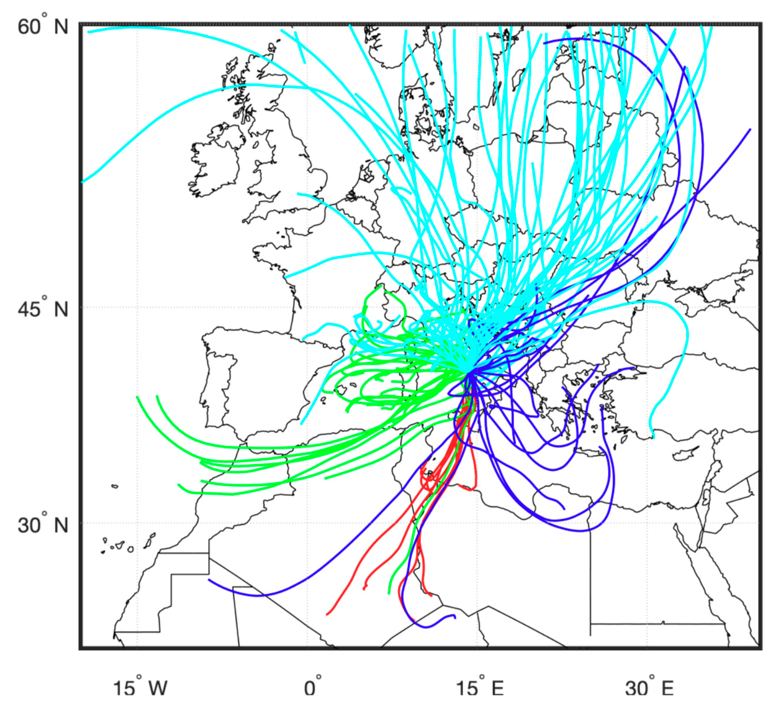
  • similar origins of the air masses, according to back-trajectories.
The origin of air masses appeared as the most discriminating parameter, which prevented the pooling of filters that had all the other features in common. Therefore, it is highlighted as the major pooling criterion and a common color code assigned to the pooled sample (see Supplementary Materials Figure S1 for a complete overview of back-trajectories related to each sample).
Once two samples were pooled together, a new vector average over the 48 h was recalculated for the wind speed and the wind direction of the pooled sample.

2.2. Sample Processing and Mass Concentration Measurements

To reduce blank levels, the filters were heated in a furnace at 700 °C for 2 h prior to sampling and stored wrapped in pre-heated (2 h at 550 °C) aluminum foil and Petri slides. To avoid volatilization, they were stored at a temperature of around −20 °C before and after sampling. For transportation they were carried in freeze bags. All tools that were used for filter handling were pre-cleaned first with acetone and then with ethanol.
Prior to 14C analysis, the EC and OC fractions were isolated on a custom-built aerosol combustion system (ACS) at the Centre for Isotopic Research (CIO-Groningen, NL) according to the two-step thermal desorption method, described by Dusek et al. [27], which was evaluated in Zenker et al. and Szidat et al. [64,65]. This method is based on the thermal method of Cachier et al. [16], which was later improved by Szidat et al. [25]. Briefly, OC is extracted by combustion in pure oxygen at 360 °C for 15 min., whereas EC is extracted at 650 °C for 15 min, after two purification steps to completely remove OC, one at 360 °C for 15 min, followed by a 2 min step at an intermediate combustion temperature of 450 °C. OC and EC are a continuum and during the intermediate step the more refractory OC and less refractory EC show similar thermochemical properties making it necessary to exclude this intermediate part of the EC for radiocarbon analysis. As a consequence, a full recovery of the EC cannot be achieved [27]. Furthermore, to minimize the charring of OC during the OC removal step, filter samples used for 14C analysis of EC have been water-extracted [64]. The CO2 evolved in the ACS system is collected cryogenically in the purification line, where contaminants such as NOx, SO2 and water vapor are removed from the sample. The extracted amount of CO2 is determined manometrically, in a calibrated volume.
The EUSAAR_2 protocol [66] was used to determine carbon mass concentrations by a thermo-optical OC-EC analyzer, manufactured by Sunset Laboratory Inc. (Model 5L). The Sunset analyzer was calibrated daily with a sucrose solution of known concentration, the instrument background was measured every day and subtracted from the measurements, flows were calibrated every half year, and the split point of OC-EC was checked visually for each sample. Concentrations of EC were measured on water extracted filter punches, since the EUSAAR_2 protocol underestimates the EC concentration on untreated samples compared to water-extracted samples. This is especially true for highly loaded filters. Dusek et al. [27] and Zenker et al. [64] tested the procedure here applied. Therefore, for detailed quantitative implications, we refer to their work, since no further testing was made for this particular study. Following their recommendation, the water-soluble carbon was removed from the filter pieces by soaking them in MilliQ water overnight (14 mL of water per filter piece) and drying them for 24 h in a desiccator over silica gel. However, due to the limited amount of sample material available, not enough filter material was left for the determination of OC concentrations, because that needs to be accomplished independently on untreated filter pieces.
Consequently, OC concentrations were derived indirectly by using OC and EC concentrations manometrically determined by the ACS and the Sunset EC measurements.
From past experiments, it has been determined that TCACS (defined as the sum of OC and EC extracted on the ACS) is very closely correlated with TC measured by the Sunset instrument (TCSUNSET), over a wide range of concentrations (see Figure S2). For 32 samples measured during these experiments, on average 69% ± 1% of the aerosol TC, measured as TCSUNSET, is recovered on the ACS. The remaining part (which is roughly 30%) is lost on the ACS during the separation step aimed at excluding the fraction, which contains the refractory OC and less refractory EC. Therefore, the OC fraction has been attained by subtraction, according to the Equation (1)
O C = TC EC = T C A C S T C S U N S E T T C A C S E C S U N S E T
where the subscript ACS stands for barometric determination of the ACS extracted fractions, Sunset for the thermo-optical measurement and TC is derived from TCACS, using the calibration factor T C S U N S E T T C A C S . The average T C S U N S E T T C A C S ratio equals 1.47 ± 0.02, over the 32 independent observations shown in the Supplementary Material Section (Figure S2).

2.3. Radiocarbon Analysis

CO2 purified and collected on the ACS system is stored in flame-sealed glass tubes until directly fed into the gas ion source of the “MIni CArbon DAting System” (MICADAS) accelerator mass spectrometer (AMS) [67] at the CIO-Groningen, NL. Usually, in aerosol science, the 14C/12C ratio in a sample is reported as fraction modern F14C [68], equivalent to the per cent Modern (pM) definition in Stuiver & Polach [69]:
F 14 C   =   ( C 14   C 12   ) s a m p l e   ( C 14   C 12   ) 1950
F14C relates the 14C/12C ratio of the sample to the ratio of the unperturbed atmosphere in the year 1950, which is defined as 0.7459 times the 14C/12C ratio of the OX-II (SRM 4990C) standard, δ13C–normalized and corrected for decay since 1950. 14C/12C ratio of the unperturbed atmosphere in the year 1950 is by definition 95% of the ratio of the original primary standard (SRM 4990B). SRM 4990B, no longer available, has been replaced by SRM 4990C, whose 14C/12C ratio is 1.2736 times the older one [70]. Isotopic fractionation during carbon assimilation from the atmosphere, sample pre-treatment and measurement is accounted for through δ13C normalization [68,69,71]. In addition, the background contamination and a small memory effect in the gas inlet of the AMS has also been corrected. The F14C measurements are routinely calibrated using the international calibration material OX-II, which is in this case combusted in similar quantities as the sample material and analyzed as CO2 gas. Background correction is performed using combusted amounts of wood of practically infinite age (which means >50,000 years in 14C terms). In addition, other reference materials, such as pure CO2 from a fossil source, and the international reference materials IAEA-C7 and IAEA-C8 are used for calibration control and accuracy assessment. F14C of OC desorbed from two “field blanks” was measured and used to correct sample data for artefacts due to organic contamination, according to Heal [32]. In all cases, the uncertainty in the calibrated F14C value of the samples due to the blank correction was negligibly small compared to the natural spread between the samples and the uncertainties caused by other steps in the analysis.

2.4. Source Apportionment

Aerosol carbon derived from presently living biomass, such as biogenic primary and secondary organic aerosols as well as aerosols from cooking or wood sprig combustion emissions, have the same F14C as the contemporary atmosphere, 1.017 ± 0.001 in the year 2016 [72], decreasing every year. Wood used for residential heating has a higher F14C, variable between 1.07 and 1.25 [29], depending on how old it is. This “bomb-spike” plant material is grown in the recent past, when the atmosphere had higher 14C levels due to the nuclear bomb tests. Fossil sources are assumed to have F14C = 0.
Following Szidat et al. [30], the following carbonaceous aerosol fractions have been quantified: ECbb (EC from biomass burning), ECff (EC from fossil fuel combustion), OCff (fossil OC) and OCnff (non-fossil OC, split into OCbb and OCother).
The concentration of ECbb is given by:
E C b b = F C 14 EC F C 14 bb E C
where F C 14 bb is the 14C content of plant materials, such as wood used for residential heating, mostly grown in the past years, under higher level of bomb-spike condition, assumed to be 1.15 ± 0.05 as in Dusek et al. [39]. Consequently, ECff is:
E C f f = E C E C b b
The concentration of the organic carbon emitted directly or indirectly by fossil sources has been quantified by the following equation:
O C f f = ( 1 F C 14 OC F C 14 p r e s e n t ) O C
where F C 14 p r e s e n t is the fraction modern of all non-fossil sources, taken as 1.08 ± 0.05 in order to account the fact that the non-fossil carbon in PM derives from multiple ‘contemporary’ sources spanning from truly contemporary, i.e., 1.017 ± 0.001 [72], to mature tree wood, i.e., F14Cbb.
Consequently, OC emitted by non-fossil fuel sources (OCnff) is:
O C n f f = O C O C f f = O C b b + O C o t h e r
while EC is directly emitted into the atmosphere by combustion processes, the OC fractions comprise both primary and secondary organic carbonaceous aerosol (SOC).
Combustion processes form most of the primary organic aerosol, together with the corresponding fraction of EC. In particular, biomass burning emits primary OC (named OCbb), whose concentration can be assessed from ECbb using an average biomass burning emission ratio (OC/EC)bb, 5 ± 2, as in Dusek et al. [39]:
O C b b = ( OC EC ) b b   E C bb
Similarly, OCff can be split into primary OC (POCff) co-emitted with ECff and the secondary fossil OC (SOCff). Following Bernardoni et al. [53], we assume that the primary emission ratio (OC/EC)ff for vehicular traffic is 1.3 ± 0.4 and derive the fossil SOCff according to Equation (8):
S O C f f = O C f f P O C f f = O C f f ( OC EC ) f f   E C ff
Subtracting OCbb from OCnff, we can finally obtain OCother:
O C o t h e r = O C n f f O C b b = O C O C f f O C b b
OCother accounts for all other contemporary (i.e., non-fossil) sources, which are not directly emitted by biomass burning. It comprises mainly biogenic or biomass burning secondary organic aerosol, cooking OC, but it can also contain primary biogenic material, which, however, in our case, in the urban environment, makes a negligible contribution to PM2.5 [39]. Under the assumption that OCother mainly derives from secondary formation, we can give a rough estimate of SOC by adding up OCother to SOCff.

2.5. Uncertainty Assessment

The partitioning model described in the previous section has been applied independently to each of the 18 samples selected for this study. This source apportionment approach consists in solving analytically a series of equations, which involves values of experimental measurements together with empirically determined parameters. At the end, the propagation of the uncertainties of both kinds of variables assesses the uncertainty associated to each fraction in each sample (reported as error bars in the figures). For most of the fixed parameters we use literature data, as reported throughout the text, and propagate the uncertainties assessed therein. The ratio TCSUNSET/TCACS, used in Equation (1) at the beginning of the chain of calculations, is determined empirically for this study. In this case, its uncertainty is assessed from the standard deviation of the TCACS residuals (±2.6 μg/cm2) from the regression line, which is forced through zero, of the experimental data correlating TCSUNSET and TCACS measurements (Figure S2). This accounts for the intrinsic variability associated with this parameter. The overall uncertainty of TC depends both on the uncertainty of TCACS (arising from temperature and pressure instrumental precision and the uncertainty of a calibrated volume) and the variability of the calibration ratio, as previously stated. TC uncertainty varies among all samples from 2% to 11% (5% on average) of the absolute value of TC. Consequently, OC concentrations calculated from TC have a slightly higher uncertainty, from 2% to 13% of the absolute value of the OC concentration (6% on average).

3. Results and Discussions

From the 24th of November 2016 until the 5th of January 2017, 18 samples (6 from a single 24 h-filter, 12 from two merged 24 h-filters) have been selected for radiocarbon measurement, covering 30 of the 42 days of the period. Table 1 gives an overview of the sampling information, such as collection date, air mass origin, meteorological parameters, as well as measured F14C of EC and OC. Meteorological parameters are from two nearby weather stations: Temperatures, wind speeds and wind directions, from Capodichino Airport (40.88° N 14.28° E, 72 m a.s.l.) [73], and precipitations, from Capodimonte (40.86° N 14.23° E, 126 m a.s.l.) [74]. During this sampling campaign, the prevailing wind direction was exclusively from the northern sector, consistent with the winter climatology of the site [75]. Air masses had mostly continental European origin (Eu. cont.) or western Mediterranean/local origin (West. Med./local). Less often the air originated from the eastern Mediterranean (East. Med.) or from the Saharan region (Saharan). No haze event occurred during this campaign, as the visibility stayed always above 6 km [76].
The 14C contribution of exogenous carbon to the OC has been taken into account by desorbing OC from “field blanks”. The “field blank” OC accounted for 3% (min 1.9%. max 7%) of the average OC load of the samples and showed a F14C of 0.597 ± 0.012, resulting in an average correction of 0.008 on the F14C. F14C of the EC has not been field-blank corrected, since EC concentrations on “field blanks” were found to be negligibly small.

3.1. PM2.5 Concentration and Composition of Its Carbonaceous Fraction

The PM2.5 concentration of each sample collected for this study is shown in Figure 3. When classified with similar air mass history, samples collected on two consecutive days have been merged, in order to optimize analysis time and costs. However, most of them have been measured separately for EC concentration, as indicated in Table 1. A weighted mean of the two measurements is assigned as EC concentration of the merged sample. They appear in the plot as two contiguous bars, with common average values associated to the pooling period. An average concentration of 29 ± 3 µg/m3 of PM2.5 was recorded. This concentration is higher than the annual average limit; fixed by law at 25 µg/m3, see Figure 3. The PM2.5 concentration reached a maximum of 68.6 ± 0.7 µg/m3 on the 10th of December 2016 (here named “pollution event”) when the air mass origin appears to be very local (see Figure S1). A minimum of 12.6 ± 0.1 µg/m3 is recorded by the last sample, in coincidence with two heavy rain events.
PM2.5 concentration stayed above the WHO recommended average concentration limit of 10 µg⁄m3 during the entire sampling period. We do not observe consistently lower PM2.5 concentrations on weekend days (striped bars in the plot), indicating that pollution sources related to workdays, such as traffic, are not dominant in determining the PM2.5 concentrations. In fact, the concentration patterns seem to be determined by a more complex combination of meteorological and source related factors. For example, comparing PM concentration to wind speed, recorded at the Capodichino Airport, it can be noticed that whenever the wind speed is very high, PM2.5 concentrations are low and the lowest wind speeds are associated to concentrations higher than average. However, for intermediate wind speeds there is not clear relationship between wind speed and PM2.5 concentrations. Low concentrations can be observed in coincidence with rain events, as reported in Table 1.
The contribution of OC and EC to PM2.5 are shown in grey and black colors, respectively. The total carbonaceous fraction of the sampled PM2.5 (in %) is indicated above each sample in Figure 3. TC accounts for 48 ± 2% of the total PM2.5 mass collected, on average. Cavalli et al. and Putaud et al. [3,5] report lower average TC to PM2.5 ratios for background rural sites in Europe: 25% and 19%, respectively. However, this ratio is shown to be very variable (from 21% to 56% across different sites and seasons), with the highest values in the months of November, December and January [5], while it is on average 33 ± 2%, if considering urban and kerbside sites in northern and central Europe [3].
Average concentrations over the whole sampling period are 12.2 ± 1.4 µg/m3 for OC and 2.2 ± 0.3 µg/m3 for EC. EC accounts for 16 ± 1% of TC, which is comparable to the findings at other European sites during the cold months, where EC contributions range from 13% to 25% [5]. The average OC/EC ratio recorded during this study (5.9 ± 0.5, ranging from 3, in coincidence with the dust event on the 24th of November, to 13, on the 31st of December) is similar to the ratio (5) reported for Budapest in winter [37], while Minguillón et al. [33] report a much smaller average value (1.7) for PM1 measured in Barcelona. OC/EC ratios of PM2.5 from different urban location in Spain, Portugal and UK range from 0.73 ± 0.25 (Lisbon, Portugal) to 4 ± 3 (Coimbra, Portugal), while higher ratios are shown at rural (in the range [4.9–5.4]) and at remote sites (in the range [9.6–13.5]) [8]. The OC/EC ratio, shown in this study, is closer to the average ratio reported by Pietrogrande et al. for a rural site (5.6 ± 0.3) than to the ratio of the urban site (3.4 ± 0.2), in northern Italy over different cold seasons [44].
Table 2 summarizes the results of the most recent literature reporting PM2.5, OC and EC concentrations, measured during cold months at different Italian sites, classified according to the closeness of the sources (urban/remote), the latitude (North/South) and the distance from the Mediterranean sea (coastal/inland). PM2.5 in Naples is in the range of other cities in Italy, whereas the carbonaceous fraction is higher than at other sites. Especially the OC concentration in Naples seems to be on the upper range of the winter concentrations for urban sites in Italy, which are on average 9 ± 1 µg/m3. On the other hand, typical urban EC concentrations, on average 1.9 ± 0.3 µg/m3, are comparable to those in Naples (Table 2). Both EC and OC concentrations are consistent with concentrations reported in the literature for the same site, measured during a previous campaign, during the same time of the year [52]. Remote sites show lower concentrations of PM2.5. Nevertheless, the TC fraction of PM2.5 tends to be comparable among different sites, and it is generally lower than in this study. TC is on average 37 ± 8% of the total PM2.5, at the remote sites cited in Table 2, and 34 ± 2%, at the urban background ones. The highest TC fractions of PM2.5 occur at near sea locations.

3.2. Fossil and Non-Fossil Contributions to EC and to OC

Figure 4 shows the fossil fractions of EC (Figure 4a) and OC (Figure 4b), projected along the prevailing wind direction represented by the vector mean for the whole sampling period. Vector colors indicate the air mass origin given in Table 1 and Figure S1. The length of each vector indicates the fossil fraction, which is also given as numbers in the figures. The wind was coming mostly from the northern sectors; therefore, it is not possible to investigate the influence of local maritime sources, such as the harbor located to the south of the sampling station. On average, the fossil fraction is 23 ± 1% and 66 ± 2% of OC and EC, respectively. Within the limited wind sector encountered during our campaign, there seems to be no particular dependence of the fossil fraction on wind direction, which might have been indicative of local sources, such as major roads. The origin of air masses, shown by different colors according to back-trajectories, does not significantly affect the fossil fractions of OC and EC. However, continental European air masses, i.e., light blue vectors, show the lowest absolute concentrations of OCff and ECff: on average 2.3 ± 0.4 µg/m3 and 1.0 ± 0.2 µg/m3, respectively. Average absolute concentrations associated to the green vectors are 3.8 ± 0.6 µg⁄m3 and 2.3 ± 0.4 µg/m3. The red vector belongs to the two filters collected from the 24th until the 26th of November 2016, when a small Saharan dust event was sampled in coincidence with rain events, which occurred on both sampling days. Just in this case, the fossil contribution appears to be higher than in all other samples, 80% of the EC fraction and 42% of the OC fraction. Absolute concentrations of OCff and ECff, in this sample, are not significantly higher than the rest (3.0 ± 0.2 µg/m3 and 2.1 ± 0.2 µg/m3, respectively).
Figure 5a shows a time series of EC concentrations split into its two components: ECbb, produced by biomass burning and ECff, from fossil fuel combustion. On average ECbb and ECff are 0.7 ± 0.1 µg⁄m3 and 1.5 ± 0.2 µg⁄m3, respectively, over the sampling period. The biomass-burning fraction of EC is 34 ± 2%, on average, i.e., burning biomass causes a substantial fraction of EC. Briggs and Long [28] reviewed EC source apportionment data published in literature since 2006 until 2014. They report the biomass-burning share of EC being in winter on average 30 ± 3%, at different European near-city stations, and 20 ± 4%, at urban stations. A number of studies have confirmed the importance of wood-burning emissions to ambient PM levels in northern and central Europe areas in wintertime, especially because of residential heating during the cold season [21,31]. Surprisingly, even at this sampling site in a coastal Mediterranean city the contribution of biomass burning to EC concentrations is significant. The biomass-burning fraction of EC does not appear to be closely related to the ambient temperature as would be expected for a residential heating source. As a matter of fact, the daily averaged ambient temperature varies from 6 °C to 16 °C during the sampling period, but no systematic increase of ECbb/EC can be noticed during the coldest days, when an enhanced use of domestic heating, even wood-fired ones, is expected. A correlation (positive or negative) between EC concentration and ambient temperature seems to be absent or very weak (see Figure S3).
Figure 5b shows OCff (fossil OC), OCbb (primary organic carbon emitted from biomass burning) and OCother (organic carbon from all other contemporary sources). On average, OCbb is 3.7 ± 0.5 µg/m3, OCother is 5.8 ± 0.8 µg/m3 and OCff is 2.7 ± 0.3 µg/m3. Contemporary (i.e., non-fossil) sources are the major fraction of OC (OCnff in Figure 5b), accounting for 77 ± 1% of the total OC. OCbb contributes considerably to this fraction and accounts on average for 31 ± 2% of OC. OCother comprises mainly biogenic or biomass burning secondary organic aerosol, and cooking OC. Its concentration is relatively uncertain, because it is very sensitive to assumptions about the primary OC/EC ratio, which can be quite variable. Comparing OCff concentrations in Naples to other European sites with similar OC concentrations during winter, we see that the coastal urban site of Aveiro (Portugal, 40° 340 N, 8° 380 W, 40 m a.s.l.) shows a lower OCff concentration (OCff is 0.2 µg/m3 at total OC concentrations of 12.3 µg/m3) [29]. However, OCff in Naples is lower than the concentration found by Gilardoni et al. [54] at a background site located at the north-western edge of the Po Valley in northern Italy (45°48’ N, 8°38’ E, 209 m a.s.l.), (OCff is 3.5 µg⁄m3 with total OC concentrations of 19 ± 10 µg/m3) [54]. The contribution of SOCff to OCff is shown in Figure 5b as a black dotted line. It varies from 4%, during the Saharan event, to 73% on the 31th of December, with an average of 30 ± 4%. SOCff generally accounts for a larger fraction of OCff for continental European air mass origin (41 ± 5%, light blue-coded back-trajectories) than for local and Mediterranean air masses (21 ± 4%, dark blue-coded and green-coded back-trajectories). In the latter case PM2.5 is dominated by local fossil sources, whereas air mass origins from northern, eastern and central Europe allow for longer aging times of the carbonaceous aerosol.
Under the assumption that OCother mainly derives from secondary formation, we can conclude that SOC is a preponderant and very variable fraction of OC, which can account for up to 80% of OC on special days, like on 31 December 2016. SOC is on average 52 ± 3% of OC. In analogy with SOCff/OCff, SOC/OC is larger for continental air mass origin (59 ± 5%), than for local and Mediterranean air masses (49 ± 2%). These findings highlight the importance of SOA formation during long-range transport in wintertime and indicate limited SOC formation in the urban area itself.
OCff and ECff are highly correlated (Figure 6). Therefore, we can assume that they have a common source, most likely vehicular traffic. The OCff/ECff ratio found in the center of Naples agrees with the OC/EC ratio of 1.3 ± 0.4 in PM2.5 samples from a tunnel study in Milan [77], which can be considered as representative for traffic primary emissions. The slope of the regression line through OCff and ECff of the samples from Naples is 1.5 ± 0.2, as shown in Figure 6, which is consistent with primary traffic emissions as the main source of OCff.
Table 3 summarizes the results of 14C-based apportionment studies for OC and EC conducted during winter campaigns at different urban sampling sites in Europe. The fraction of EC emitted by fossil sources varies from the 17% in Aveiro (Portugal) to roughly 90% in Birmingham and Goteborg. OCff/OC shows a narrower range of variability (20 to 44%). The fossil contribution to both particle fractions is in Naples on the lower side of these ranges. In particular, a higher influence of fossil sources than in Naples is noticed in Milan [53], which is, to our knowledge, the only other urban site in Italy where this kind of investigation is accomplished. There is just one more 14C source apportionment study published about Italian sites. It refers to Ispra, which is a remote site, here reported for completeness, notwithstanding its different nature as compared to the other examples listed in Table 3. Despite its remote location, the share of airborne fossil carbon particles at Ispra is just slightly lower than in the city of Naples [54].

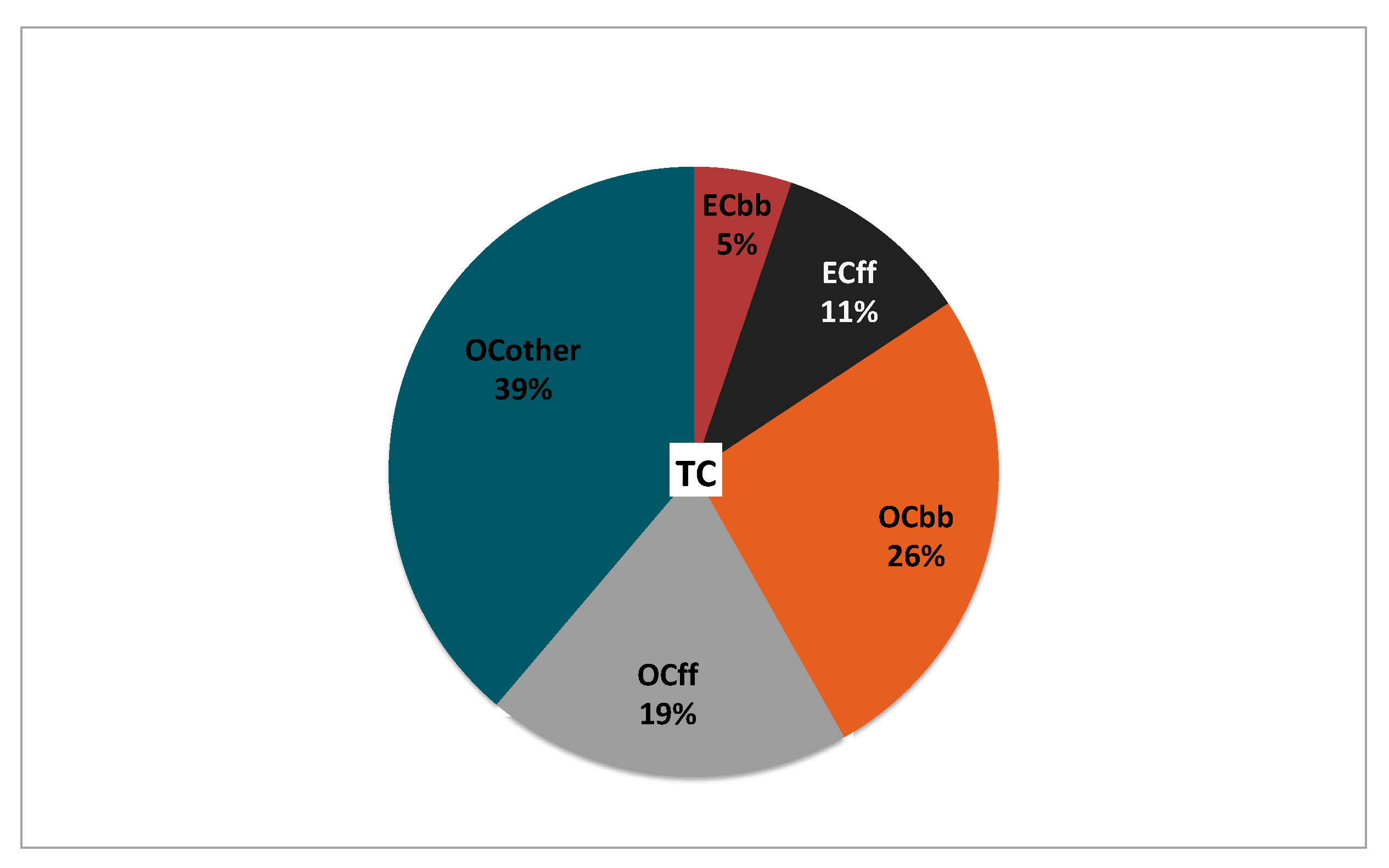
3.3. Source Apportionment of TC and Associated Uncertainties

The source contributions to OC and EC, assessed by the methods reported above, were merged to obtain an average of the different source’s inputs to total carbon (Figure 7).
TC, roughly half of PM2.5 mass, is predominantly (70% of TC) produced by non-fossil sources (i.e., biomass burning, biogenic emissions etc.). A similar scenario is reported during winter-smog episodes for locations around the Alps, where non-fossil carbon equals about three quarters of the total carbon [21]. However, the contribution of non-fossil sources varies considerably during the reported period, being as low as 47 ± 8%, during the first sampling day, and up to 81 ± 6%, on the two days starting on the 19th of December, being on average 70 ± 1% (weighted mean according to data uncertainties ± associated error). Furthermore, this fraction is very sensitive to the parameters F14Cbb and F14Cpresent (assumed to be the mean value between F14Cbb and the F14C of the contemporary atmosphere). Under the assumptions that F14Cbb is set to the highest limit of the range reported in literature (i.e., 1.20) and F14Cpresent is taken equal to F14Cbb, the weighted mean of non-fossil sources contribution to TC becomes 64 ± 1%, while it is 75 ± 2%, when taking the lowest limit for F14Cbb (i.e., 1.15) and by assuming that F14Cpresent is exactly that of the contemporary atmosphere (1.02 for year 2016 [72]).
Primary biomass burning carbon (OCbb + ECbb) alone is 31% of TC, i.e., 15% of the PM2.5 mass. Therefore, fossil fuel sources produce, directly or indirectly, less than one third of TC, i.e., 14% of PM2.5 mass, whereas higher fossil contributions are reported both near the Mediterranean city of Athens (Greece) and at Odense (Denmark), 54% and 59% of TC, respectively [41].
From the uncertainty assessment described in Section 2.5, we estimate typical relative errors of ±5%, for ECff/TC (varying from ±0.002 to ±0.013, as absolute errors); ±19% for OCff/TC (varying from ±0.03 to ±0.05); ±14% for ECbb/TC (varying from ±0.003 to ±0.015); ±43% for OCbb/TC (varying from ±0.06 to ±0.17) and ±9% for OCother/TC (varying from ±0.09 to ±0.19). The values in Figure 7, which are affected by higher uncertainties, are those derived by longer chains of calculations. As compared to a similar study conducted in Italy [53], our uncertainties are bigger, mainly because of indirect determination of TC and OC concentrations, due to a lack of sufficient amount of sample material.

4. Conclusions

In Naples during wintertime, TC accounts for 48% of the total PM2.5, which is higher than at other urban locations in Italy. Considering that PM2.5 also contains a significant mass fraction from natural contributions (such as sea salts), as indicated by other studies focusing on ionic composition of fine particles in Naples [59], carbonaceous materials are a very important component of PM2.5.
On average 29% of the total carbon (i.e., less than 15% of the total PM2.5) originates from fossil sources. Fossil sources are the dominant fraction of EC (66%), but a much smaller fraction of OC (23%). The biomass contribution (34%) to EC is higher than expected in comparison with other large urban locations [31,32,53], where a range of 9% to 23% modern carbon in EC is reported. For an urban location, not only the ratio ECbb/EC, but also the overall contribution of primary biomass burning carbon (i.e., OCbb + ECbb) to the ambient aerosol is relatively high, accounting for 15% of PM2.5. The absence of a clear correlation of biomass burning carbon fraction with ambient temperature indicates that residential heating might not be the main source of biomass burning emissions, pointing to potential other sources, such as, for example, cooking on wood fires. However, further investigations such as improving the knowledge on OC/EC emission ratios of the local sources and seasonal comparisons are needed to shed more light on this aspect. Therefore, studies on typical sources (emission ratios and signatures) and more extensive campaigns, extending the monitoring time to different seasons or considering diurnal variations, are necessary and desirable in this area. In particular, non-fossil sources contribution to TC is sensitive to the 14C signature attributed to biomass burning. The weighted mean of non-fossil sources contribution to TC, over the investigated period, varies from 64 ± 1% to 75 ± 2%, depending on the different assumptions taken from the literature, which refer generally to European data. Using the 14C signature of emission sources measured under local conditions would reduce this uncertainty.
However, despite uncertainties, the results of this initial study show how a better knowledge of the local and regional sources and of the PM accumulation patterns can give indications towards reducing fine particle concentrations in order to meet the legal requirements, for better air quality in urban areas. After all, blaming the nature of the low urban air quality in Naples merely on vehicular traffic belittles the problem, since roughly two third of TC, which is half of PM2.5, comes from non-fossil sources. Measures to improve air quality should go beyond traffic bans during pollution peaks or traffic restrictions in confined city-zones, as other emission sources, such as biomass burning or secondary aerosol formation, play a more significant role in the high concentration of the fine particles.

Supplementary Materials

The following are available online at https://www.mdpi.com/2073-4433/10/8/451/s1, Figure S1: Back trajectories. For every sampled filter, 6-h back trajectories have been calculated, using Hybrid Single-Particle Lagrangian Integrated Trajectory (HYSPLIT) model, Figure S2: Deriving the correction factor TCSunset/TCACS, Figure S3: ECbb/EC in comparison with average ambient temperature, during the sampling time.

Author Contributions

Conceptualization, C.S. and U.D.; data curation, C.S.; Formal analysis, C.S. and A.R.; funding acquisition, A.D’.O. and H.A.J.M.; investigation, C.S., A.R., E.C., H.N. and K.Z.; resources, H.A.J.M.; supervision, U.D.; visualization, C.S.; writing—original draft, C.S.; writing—review & editing, C.S., A.R., E.C., H.N., K.Z., A.D’.O., H.A.J.M. and U.D.

Funding

This research received no external funding.

Acknowledgments

The authors thank an anonymous referee for the suggested improvements. Carmina Sirignano is in debt to Antonio Petraglia and Mauro Rubino for their suggestions, the fruitful discussions and the proofreading during the preparation of this work.

Conflicts of Interest

The authors declare no conflict of interest.

References

  1. Fuzzi, S.; Baltensperger, U.; Carslaw, K.; Decesari, S.; Denier van der Gon, H.; Facchini, M.C.; Fowler, D.; Koren, I.; Langford, B.; Lohmann, U.; et al. Particulate matter, air quality and climate: Lessons learned and future needs. Atmos. Chem. Phys. 2015, 15, 8217–8299. [Google Scholar] [CrossRef]
  2. Liang, C.S.; Duan, F.K.; He, K.-B.; Ma, Y.L. Review on recent progress in observations, source identifications and countermeasures of PM2.5. Environ. Int. 2016, 86, 150–170. [Google Scholar] [CrossRef] [PubMed]
  3. Putaud, J.P.; van Dingenen, R.; Alastuey, A.; Bauer, H.; Birmili, W.; Cyrys, J.; Flentje, H.; Fuzzi, S.; Gehrig, R.; Hansson, H.C.; et al. A European aerosol phenomenology—3: Physical and chemical characteristics of particulate matter from 60 rural, urban, and kerbside sites across Europe. Atmos. Environ. 2010, 44, 1308–1320. [Google Scholar] [CrossRef]
  4. Jacobson, M.C.; Hansson, H.-C.; Noone, K.J.; Charlson, R.J. Organic atmospheric aerosols: Review and state of the science. Rev. Geophys. 2000, 38, 267–294. [Google Scholar] [CrossRef] [Green Version]
  5. Cavalli, F.; Alastuey, A.; Areskoug, H.; Ceburnis, D.; Čech, J.; Genberg, J.; Harrison, R.M.; Jaffrezo, J.L.; Kiss, G.; Laj, P.; et al. A European aerosol phenomenology-4: Harmonized concentrations of carbonaceous aerosol at 10 regional background sites across Europe. Atmos. Environ. 2016, 144, 133–145. [Google Scholar] [CrossRef]
  6. Petzold, A.; Ogren, J.A.; Fiebig, M.; Laj, P.; Li, S.M.; Baltensperger, U.; Holzer-Popp, T.; Kinne, S.; Pappalardo, G.; Sugimoto, N.; et al. Recommendations for reporting black carbon measurements. Atmos. Chem. Phys. 2013, 13, 8365–8379. [Google Scholar] [CrossRef]
  7. Turpin, B.J.; Huntzicker, J.J. Identification of secondary organic aerosol episodes and quantitation of primary and secondary organic aerosol concentrations during SCAQS. Atmos. Environ. 1995, 29, 3527–3544. [Google Scholar] [CrossRef]
  8. Pio, C.; Cerqueira, M.; Harrison, R.M.; Nunes, T.; Mirante, F.; Alves, C.; Oliveira, C.; Sanchez de la Campa, A.; Artíñano, B.; Matos, M. OC/EC ratio observations in Europe: Re-thinking the approach for apportionment between primary and secondary organic carbon. Atmos. Environ. 2011, 45, 6121–6132. [Google Scholar] [CrossRef]
  9. Wu, C.; Yu, J.Z. Determination of primary combustion source organic carbon-to-elemental carbon (OC/EC) ratio using ambient OC and EC measurements: Secondary OC-EC correlation minimization method. Atmos. Chem. Phys. 2016, 16, 5453–5465. [Google Scholar] [CrossRef]
  10. World Health Organization. Review of Evidence on Health Aspects of Air Pollution—REVIHAAP Project; World Health Organization: Copenhagen, Denmark, 2013. [Google Scholar]
  11. Landrigan, P.J.; Fuller, R.; Acosta, N.J.R.; Adeyi, O.; Arnold, R.; Basu, N.; Baldé, A.B.; Bertollini, R.; Bose-O’Reilly, S.; Boufford, J.I.; et al. The Lancet Commission on pollution and health. Lancet 2018, 391, 462–512. [Google Scholar] [CrossRef] [Green Version]
  12. Boucher, O.; Randall, D.; Artaxo, P.; Bretherton, C.; Feingold, G.; Forster, P.V.-M.; Kerminen, Y.; Kondo, H.; Liao, U.; Lohmann, P.; et al. Clouds and Aerosols. In Climate Change 2013—The Physical Science Basis; Contribution of Working Group I to the Fifth Assessment Report of the Intergovernmental Panel on Climate Change; Stocker, T.F., Qin, D., Plattner, G.-K., Tignor, M., Allen, S.K., Boschung, J., Nauels, A., Xia, Y., Bex, V., Midgley, P.M., Eds.; Cambridge University Press: Cambridge, UK; New York, NY, USA, 2013. [Google Scholar]
  13. World Health Organization. Ambient (Outdoor) Air Quality and Health. Available online: http://www.who.int/mediacenter/factsheets/fs313/en/ (accessed on 20 January 2018).
  14. Viana, M.; Kuhlbusch, T.A.J.; Querol, X.; Alastuey, A.; Harrison, R.M.; Hopke, P.K.; Winiwarter, W.; Vallius, M.; Szidat, S.; Prévôt, A.S.H.; et al. Source apportionment of particulate matter in Europe: A review of methods and results. J. Aerosol Sci. 2008, 39, 827–849. [Google Scholar] [CrossRef]
  15. Currie, L.A.; Klouda, G.A.; Continetti, R.E.; Kaplan, I.R.; Wong, W.W.; Dzubay, T.G.; Stevens, R.K. On the Origin of Carbonaceous Particles in American Cities: Results of Radiocarbon “Dating” and Chemical Characterization. Radiocarbon 1983, 25, 603–614. [Google Scholar] [CrossRef]
  16. Cachier, H.; Bremond, M.; Buat-Ménard, P. Determination of atmospheric soot carbon with a simple thermal method. Tellus B Chem. Phys. Meteorol. 1989, 41, 379–390. [Google Scholar] [CrossRef]
  17. Currie, L.A. Evolution and Multidisciplinary Frontiers of 14 C Aerosol Science. Radiocarbon 2000, 42, 115–126. [Google Scholar] [CrossRef]
  18. Szidat, S.; Jenk, T.M.; Gäggeler, H.; Synal, H.-A.; Fisseha, R.; Baltensperger, U.; Kalberer, M.; Samburova, V.; Reimann, S.; Kasper-Giebl, A.; et al. Radiocarbon (14C)-deduced biogenic and anthropogenic contributions to organic carbon (OC) of urban aerosols from Zürich, Switzerland. Atmos. Environ. 2004, 38, 4035–4044. [Google Scholar] [CrossRef]
  19. Ceburnis, D.; Garbaras, A.; Szidat, S.; Rinaldi, M.; Fahrni, S.; Perron, N.; Wacker, L.; Leinert, S.; Remeikis, V.; Facchini, M.C.; et al. Quantification of the carbonaceous matter origin in submicron marine aerosol by 13C and 14C isotope analysis. Atmos. Chem. Phys. 2011, 11, 8593–8606. [Google Scholar] [CrossRef] [Green Version]
  20. Heal, M.R. The application of carbon-14 analyses to the source apportionment of atmospheric carbonaceous particulate matter: A review. Anal. Bioanal. Chem. 2014, 406, 81–98. [Google Scholar] [CrossRef]
  21. Zotter, P.; Ciobanu, V.G.; Zhang, Y.L.; El-Haddad, I.; Macchia, M.; Daellenbach, K.R.; Salazar, G.A.; Huang, R.-J.; Wacker, L.; Hueglin, C.; et al. Radiocarbon analysis of elemental and organic carbon in Switzerland during winter-smog episodes from 2008 to 2012—Part 1: Source apportionment and spatial variability. Atmos. Chem. Phys. 2014, 14, 13551–13570. [Google Scholar] [CrossRef]
  22. Garbarienė, I.; Šapolaitė, J.; Garbaras, A.; Ežerinskis, Ž.; Pocevičius, M.; Krikščikas, L.; Plukis, A.; Remeikis, V. Origin Identification of Carbonaceous Aerosol Particles by Carbon Isotope Ratio Analysis. Aerosol Air Qual. Res. 2016, 16, 1356–1365. [Google Scholar] [CrossRef] [Green Version]
  23. Ni, H.; Tian, J.; Wang, X.; Wang, Q.; Han, Y.; Cao, J.; Long, X.; Chen, L.W.A.; Chow, J.C.; Watson, J.G.; et al. PM2.5 emissions and source profiles from open burning of crop residues. Atmos. Environ. 2017, 169, 229–237. [Google Scholar] [CrossRef]
  24. Ni, H.; Huang, R.J.; Cao, J.; Liu, W.; Zhang, T.; Wang, M.; Meijer, H.A.J.; Dusek, U. Source apportionment of carbonaceous aerosols in Xi’an, China: Insights from a full year of measurements of radiocarbon and the stable isotope 13C. Atmos. Chem. Phys. 2018, 18, 16363–16383. [Google Scholar] [CrossRef]
  25. Szidat, S.; Jenk, T.M.; Gäggeler, H.; Synal, H.-A.; Hajdas, I.; Bonani, G.; Saurer, M. THEODORE, a two-step heating system for the EC/OC determination of radiocarbon (14C) in the environment. Nucl. Instrum. Methods Phys. Res. Sect. B Beam Interact. Mater. Atoms 2004, 223, 829–836. [Google Scholar] [CrossRef]
  26. Calzolai, G.; Bernardoni, V.; Chiari, M.; Fedi, M.E.; Lucarelli, F.; Nava, S.; Riccobono, F.; Taccetti, F.; Valli, G.; Vecchi, R. The new sample preparation line for radiocarbon measurements on atmospheric aerosol at LABEC. Nucl. Instrum. Methods Phys. Res. Sect. B Beam Interact. Mater. Atoms 2011, 269, 203–208. [Google Scholar] [CrossRef]
  27. Dusek, U.; Monaco, M.; Prokopiou, M.; Gongriep, F.; Hitzenberger, R.; Meijer, H.A.J.; Röckmann, T. Evaluation of a two-step thermal method for separating organic and elemental carbon for radiocarbon analysis. Atmos. Meas. Tech. 2014, 7, 1943–1955. [Google Scholar] [CrossRef] [Green Version]
  28. Briggs, N.L.; Long, C.M. Critical review of black carbon and elemental carbon source apportionment in Europe and the United States. Atmos. Environ. 2016, 144, 409–427. [Google Scholar] [CrossRef]
  29. Gelencsér, A.; May, B.; Simpson, D.; Sánchez-Ochoa, A.; Kasper-Giebl, A.; Puxbaum, H.; Caseiro, A.; Pio, C.A.C.; Legrand, M. Source apportionment of PM2.5 organic aerosol over Europe: Primary/secondary, natural/anthropogenic, and fossil/biogenic origin. J. Geophys. Res. 2007, 112, D23S04. [Google Scholar] [CrossRef]
  30. Szidat, S.; Jenk, T.M.; Synal, H.-A.; Kalberer, M.; Wacker, L.; Hajdas, I.; Kasper-Giebl, A.; Baltensperger, U. Contributions of fossil fuel, biomass-burning, and biogenic emissions to carbonaceous aerosols in Zurich as traced by 14C. J. Geophys. Res. Atmos. 2006, 111, 111. [Google Scholar] [CrossRef]
  31. Szidat, S.; Ruff, M.; Perron, N.; Wacker, L.; Synal, H.-A.; Hallquist, M.; Shannigrahi, A.S.; Yttri, K.E.; Dye, C.; Simpson, D. Fossil and non-fossil sources of organic carbon (OC) and elemental carbon (EC) in Göteborg, Sweden. Atmos. Chem. Phys. 2009, 9, 1521–1535. [Google Scholar] [CrossRef]
  32. Heal, M.R.; Naysmith, P.; Cook, G.T.; Xu, S.; Duran, T.R.; Harrison, R.M. Application of 14C analyses to source apportionment of carbonaceous PM2.5 in the UK. Atmos. Environ. 2011, 45, 2341–2348. [Google Scholar] [CrossRef] [Green Version]
  33. Minguillón, M.C.; Perron, N.; Querol, X.; Szidat, S.; Fahrni, S.M.; Alastuey, A.; Jimenez, J.L.; Mohr, C.; Ortega, A.M.; Day, D.A.; et al. Fossil versus contemporary sources of fine elemental and organic carbonaceous particulate matter during the DAURE campaign in Northeast Spain. Atmos. Chem. Phys. 2011, 11, 12067–12084. [Google Scholar] [CrossRef] [Green Version]
  34. Yttri, K.E.; Simpson, D.; Stenstr, K.; Puxbaum, H.; Svendby, T. Source apportionment of the carbonaceous aerosol in Norway—quantitative estimates based on 14 C, thermal-optical and organic tracer analysis. Atmos. Chem. Phys. 2011, 11, 9375–9394. [Google Scholar] [CrossRef]
  35. Keuken, M.P.; Moerman, M.; Voogt, M.; Blom, M.; Weijers, E.P.; Röckmann, T.; Dusek, U. Source contributions to PM2.5 and PM10 at an urban background and a street location. Atmos. Environ. 2013, 71, 26–35. [Google Scholar] [CrossRef] [Green Version]
  36. Zhang, Y.L.; Zotter, P.; Perron, N.; Prévôt, A.S.H.; Wacker, L.; Szidat, S. Fractions in Fine and Coarse Particles by Radiocarbon Measurement. Radiocarbon 2013, 55, 1510–1520. [Google Scholar] [CrossRef]
  37. Salma, I.; Németh, Z.; Weidinger, T.; Maenhaut, W.; Claeys, M.; Molnár, M.; Major, I.; Ajtai, T.; Utry, N.; Bozóki, Z. Source apportionment of carbonaceous chemical species to fossil fuel combustion, biomass burning and biogenic emissions by a coupled radiocarbon-levoglucosan marker method. Atmos. Chem. Phys. 2017, 17, 13767–13781. [Google Scholar] [CrossRef]
  38. Dusek, U.; Brink, H.M.T.; Meijer, H.A.J.; Kos, G.; Mrozek, D.; Röckmann, T.; Holzinger, R.; Weijers, E.P.; ten Brink, H.M.; Meijer, H.A.J.; et al. The contribution of fossil sources to the organic aerosol in the Netherlands. Atmos. Environ. 2013, 74, 169–176. [Google Scholar] [CrossRef] [Green Version]
  39. Dusek, U.; Hitzenberger, R.; Kasper-Giebl, A.; Kistler, M.; Meijer, H.A.J.; Szidat, S.; Wacker, L.; Holzinger, R.; Röckmann, T. Sources and formation mechanisms of carbonaceous aerosol at a regional background site in the Netherlands: Insights from a year-long radiocarbon study. Atmos. Chem. Phys. 2017, 17, 3233–3251. [Google Scholar] [CrossRef]
  40. Glasius, M.; Hansen, A.M.K.; Claeys, M.; Henzing, J.S.; Jedynska, A.D.; Kasper-Giebl, A.; Kistler, M.; Kristensen, K.; Martinsson, J.; Maenhaut, W.; et al. Composition and sources of carbonaceous aerosols in Northern Europe during winter. Atmos. Environ. 2018, 173, 127–141. [Google Scholar] [CrossRef]
  41. Glasius, M.; La Cour, A.; Lohse, C. Fossil and nonfossil carbon in fine particulate matter: A study of five European cities. J. Geophys. Res. Atmos. 2011, 116, 1–11. [Google Scholar] [CrossRef]
  42. Sandrini, S.; Fuzzi, S.; Piazzalunga, A.; Prati, P.; Bonasoni, P.; Cavalli, F.; Bove, M.C.; Calvello, M.; Cappelletti, D.; Colombi, C.; et al. Spatial and seasonal variability of carbonaceous aerosol across Italy. Atmos. Environ. 2014, 99, 587–598. [Google Scholar] [CrossRef]
  43. Costabile, F.; Alas, H.; Aufderheide, M.; Avino, P.; Amato, F.; Argentini, S.; Barnaba, F.; Berico, M.; Bernardoni, V.; Biondi, R.; et al. First results of the “Carbonaceous Aerosol in Rome and Environs (CARE)” Experiment: Beyond current standards for PM10. Atmosphere 2017, 8, 249. [Google Scholar] [CrossRef]
  44. Pietrogrande, M.C.; Bacco, D.; Ferrari, S.; Ricciardelli, I.; Scotto, F.; Trentini, A.; Visentin, M. Characteristics and major sources of carbonaceous aerosols in PM2.5 in Emilia Romagna Region (Northern Italy) from four-year observations. Sci. Total Environ. 2016, 553, 172–183. [Google Scholar] [CrossRef]
  45. Khan, M.B.; Masiol, M.; Formenton, G.; Di Gilio, A.; de Gennaro, G.; Agostinelli, C.; Pavoni, B. Carbonaceous PM2.5 and secondary organic aerosol across the Veneto region (NE Italy). Sci. Total Environ. 2016, 542, 172–181. [Google Scholar] [CrossRef] [PubMed]
  46. Ricciardelli, I.; Bacco, D.; Rinaldi, M.; Bonafè, G.; Scotto, F.; Trentini, A.; Bertacci, G.; Ugolini, P.; Zigola, C.; Rovere, F.; et al. A three-year investigation of daily PM2.5 main chemical components in four sites: The routine measurement program of the Supersito Project (Po Valley, Italy). Atmos. Environ. 2017, 152, 418–430. [Google Scholar] [CrossRef]
  47. Costa, V.; Bacco, D.; Castellazzi, S.; Ricciardelli, I.; Vecchietti, R.; Zigola, C.; Pietrogrande, M.C. Characteristics of carbonaceous aerosols in Emilia-Romagna (Northern Italy) based on two fall/winter field campaigns. Atmos. Res. 2016, 167, 100–107. [Google Scholar] [CrossRef]
  48. Contini, D.; Vecchi, R.; Viana, M. Carbonaceous aerosols in the atmosphere. Atmosphere 2018, 9, 181. [Google Scholar] [CrossRef]
  49. Siciliano, T.; Siciliano, M.; Malitesta, C.; Proto, A.; Cucciniello, R.; Giove, A.; Iacobellis, S.; Genga, A. Carbonaceous PM10 and PM2.5 and secondary organic aerosol in a coastal rural site near Brindisi (Southern Italy). Environ. Sci. Pollut. Res. 2018, 25, 23929–23945. [Google Scholar] [CrossRef] [PubMed]
  50. Cesari, D.; Merico, E.; Dinoi, A.; Marinoni, A.; Bonasoni, P.; Contini, D. Seasonal variability of carbonaceous aerosols in an urban background area in Southern Italy. Atmos. Res. 2018, 200, 97–108. [Google Scholar] [CrossRef]
  51. Cesari, D.; De Benedetto, G.E.; Bonasoni, P.; Busetto, M.; Dinoi, A.; Merico, E.; Chirizzi, D.; Cristofanelli, P.; Donateo, A.; Grasso, F.M.; et al. Seasonal variability of PM2.5 and PM10 composition and sources in an urban background site in Southern Italy. Sci. Total Environ. 2018, 612, 202–213. [Google Scholar] [CrossRef]
  52. Dinoi, A.; Cesari, D.; Marinoni, A.; Bonasoni, P.; Riccio, A.; Chianese, E.; Tirimberio, G.; Naccarato, A.; Sprovieri, F.; Andreoli, V.; et al. Inter-Comparison of Carbon Content in PM2.5 and PM10 Collected at Five Measurement Sites in Southern Italy. Atmosphere 2017, 8, 243. [Google Scholar] [CrossRef]
  53. Bernardoni, V.; Calzolai, G.; Chiari, M.; Fedi, M.; Lucarelli, F.; Nava, S.; Piazzalunga, A.; Riccobono, F.; Taccetti, F.; Valli, G.; et al. Radiocarbon analysis on organic and elemental carbon in aerosol samples and source apportionment at an urban site in Northern Italy. J. Aerosol Sci. 2013, 56, 88–99. [Google Scholar] [CrossRef]
  54. Gilardoni, S.; Vignati, E.; Cavalli, F.; Putaud, J.P.; Larsen, B.R.; Karl, M.; StenstrÃm, K.; Genberg, J.; Henne, S.; Dentener, F. Better constraints on sources of carbonaceous aerosols using a combined 14C-macro tracer analysis in a European rural background site. Atmos. Chem. Phys. 2011, 11, 5685–5700. [Google Scholar] [CrossRef]
  55. Eurostat Population Density by Metropolitan Regions. Available online: http://appsso.eurostat.ec.europa.eu/nui/submitViewTableAction.do (accessed on 9 May 2018).
  56. Cattani, G.; Di Menno di Bucchianico, A.; Gaeta, A.; Leone, G. QUALITÀ DELL’ ARIA. In XIII Rapporto Qualità Dell’ambiente Urbano; ISPRA Istituto Superiore per la Protezione e la Ricerca Ambientale: Rome, Italy, 2017; ISBN 9788844808587. [Google Scholar]
  57. European Parliament and Council. Directive (EU) 2016/2284 of the european parliament and of the council of 14 December 2016 on on the reduction of national emissions of certain atmospheric pollutants, amending Directive 2003/35/EC and repealing Directive 2001/81/EC. Off. J. Eur. Union 2016, 344, 1–31. [Google Scholar]
  58. Di Vaio, P.; Magli, E.; Barbato, F.; Caliendo, G.; Cocozziello, B.; Corvino, A.; De Marco, A.; Fiorino, F.; Frecentese, F.; Onorati, G.; et al. Chemical composition of PM10at urban sites in Naples (Italy). Atmosphere 2016, 7, 163. [Google Scholar] [CrossRef]
  59. Riccio, A.; Chianese, E.; Agrillo, G.; Esposito, C.; Ferrara, L.; Tirimberio, G. Source apportion of atmospheric particulate matter: A joint Eulerian/Lagrangian approach. Environ. Sci. Pollut. Res. 2014, 21, 13160–13168. [Google Scholar] [CrossRef] [PubMed]
  60. Riccio, A.; Chianese, E.; Monaco, D.; Costagliola, M.A.; Perretta, G.; Prati, M.V.; Agrillo, G.; Esposito, A.; Gasbarra, D.; Shindler, L.; et al. Real-world automotive particulate matter and PAH emission factors and profile concentrations: Results from an urban tunnel experiment in Naples, Italy. Atmos. Environ. 2016, 141, 379–387. [Google Scholar] [CrossRef]
  61. Riccio, A.; Chianese, E.; Tirimberio, G.; Prati, M.V. Emission factors of inorganic ions from road traffic: A case study from the city of Naples (Italy). Transp. Res. Part D Transp. Environ. 2017, 54, 239–249. [Google Scholar] [CrossRef]
  62. Draxler, R.R.; Rolph, G.D. HYSPLIT (HYbrid Single-Particle Lagrangian Integrated Trajectory). Available online: http://www.arl.noaa.gov/HYSPLIT.php (accessed on 9 June 2019).
  63. Grange, S.K. Technical Note: Averaging Wind Speeds and Directions. Available online: http://rgdoi.net/10.13140/RG.2.1.3349.2006 (accessed on 9 June 2019).
  64. Zenker, K.; Vonwiller, M.; Szidat, S.; Calzolai, G.; Giannoni, M.; Bernardoni, V.; Jedynska, A.D.; Henzing, B.; Meijer, H.A.J.; Dusek, U. Evaluation and Inter-Comparison of Oxygen-Based OC-EC Separation Methods for Radiocarbon Analysis of Ambient Aerosol Particle Samples. Atmosphere 2017, 8, 226. [Google Scholar] [CrossRef]
  65. Szidat, S.; Bench, G.; Bernardoni, V.; Calzolai, G.; Czimczik, C.I.; Derendorp, L. Intercomparison of 14C Analysis of Carbonaceous Aerosols: Exercise 2009. Radiocarbon 2013, 55, 1496–1509. [Google Scholar] [CrossRef] [Green Version]
  66. Cavalli, F.; Viana, M.; Yttri, K.E.; Genberg, J.; Putaud, J.P. Toward a standardised thermal-optical protocol for measuring atmospheric organic and elemental carbon: The EUSAAR protocol. Atmos. Meas. Tech. 2010, 3, 79–89. [Google Scholar] [CrossRef]
  67. Synal, H.A.; Stocker, M.; Suter, M. MICADAS: A new compact radiocarbon AMS system. Nucl. Instrum. Methods Phys. Res. Sect. B Beam Interact. Mater. Atoms 2007, 259, 7–13. [Google Scholar] [CrossRef]
  68. Reimer, P.J.; Brown, T.A.; Reimer, R.W. Discussion: Reporting and Calibration of Post-Bomb 14C Data. Radiocarbon 2004, 46, 1299–1304. [Google Scholar]
  69. Stuiver, M.; Polach, H.A. Discussion: Reporting of 14 C data. Radiocarbon 1977, 19, 355–363. [Google Scholar] [CrossRef]
  70. Mann, W.B.W.B. An international reference material for radiocarbon dating. Radiocarbon 1983, 25, 519–527. [Google Scholar] [CrossRef]
  71. Mook, W.G.; Plicht, J.V.D. Reporting 14C Activities and Concentrations. Radiocarbon 1999, 41, 227–239. [Google Scholar] [CrossRef]
  72. Hammer, S.; Levin, I. Monthly mean atmospheric D14CO2 at Jungfraujoch and Schauinsland from 1986 to 2016. heiDATA 2017. [Google Scholar] [CrossRef]
  73. NOAA MADIS (Metorological Assimilation Data Ingest System). Available online: https://madis.ncep.noaa.gov (accessed on 11 February 2018).
  74. Centrofunzionale Multirischi della Protezione Civile Regione Campania Archivio Pluviometrici. Available online: http://centrofunzionale.regione.campania.it/#/pages/sensori/archivio-pluviometrici (accessed on 9 June 2019).
  75. Petrarca, S.; Spinelli, F.; Cogliani, E.; Mancini, M. Profilo Climatico dell’Italia; ENEA: Rome, Italy, 1999; Volume 6, ISBN 88-8286-081-7. [Google Scholar]
  76. Ilmeteo Archivio-Meteo Napoli. Available online: https://www.ilmeteo.it/portale/archivio-meteo/Napoli (accessed on 1 June 2018).
  77. Giugliano, M.; Lonati, G.; Butelli, P.; Romele, L.; Tardivo, R.; Grosso, M. Fine particulate (PM2.5-PM1) at urban sites with different traffic exposure. Atmos. Environ. 2005, 39, 2421–2431. [Google Scholar] [CrossRef]
Figure 1. Location of the sampling site in Naples (Italy).
Atmosphere 10 00451 g001
Figure 2. Back-trajectories relative to the days of interest, calculated with the HYSPLIT model.
Atmosphere 10 00451 g002
Figure 3. PM2.5 concentrations, as total (full height bars) and its fractions: OC (grey), EC (black) and all other species not bearing carbon (light blue). The TC fraction of total PM has been reported on the plot for each sample as black figures (%). Average wind speed has been reported on the secondary scale for comparison. Weekend days have been highlighted by stripes on the bars.
Atmosphere 10 00451 g003
Figure 4. (a). The fossil share of EC projected along to the prevailing wind direction during the sampling time. Each vector lays on the average wind direction. Vector colors follow the origin code assigned according to back-trajectories and the length of each vector corresponds to the fossil fraction, given also in numbers. (b) As for Figure 4a, but for OCff.
Atmosphere 10 00451 g004
Figure 5. (a). Radiocarbon-based partitioning of the EC fraction. Black bars are for ECff, and brown bars for ECbb. Error bars result by propagating uncertainties of literature parameters and observations. The fraction of EC due to biomass burning is reported in brown numbers for each sample (a dotted brown line is plotted on an arbitrary scale and guides the eyes). Mean temperature during the period covered by each sample is reported as green triangles and referred to the secondary scale of the plot. (b). As for Figure 5a, black and brown bars are for fossil fuel and biomass burning components, respectively. Teal blue bars show OCother, i.e., the OC fraction that is non-fossil and not attributable to biomass burning. Green figures (dotted green line to guide the eyes) give the sum of the fractions of the OC emitted directly and formed by secondary processes by all modern sources, i.e., OCbb/OC + OCother/OC. The share of OCff derived from secondary emissions (SOCff/OCff) is given in black numbers for each sample (dotted black line to guide the eyes).
Atmosphere 10 00451 g005
Figure 6. Correlation between OCff and ECff, in the city center of Naples. Solid line is the regression line through the observations. Dotted lines resemble primary vehicular traffic emissions simulated by accounting emission ratio (OC/EC)ff in the range from 0.9 to 1.7, as reported in literature. Peculiar sampling days have been shown with different symbols and labelled.
Atmosphere 10 00451 g006
Figure 7. Summary of partitioning results. PM2.5 carbonaceous fractions, i.e., TC, split into different sources according to the 14C-based source apportionment.
Atmosphere 10 00451 g007
Table 1. Sampling information. Samples have been identified with a serial number from 1 to 18 (N), the date of the first sampling day (Start date), air masses origin according to back-trajectories (Origin), color code (C_code), the number of days covered by each sample (# days). Basic meteorological parameters are from the Capodichino Airport: average daily temperatures (T), average wind speeds (wind speed) and prevailing wind directions (wind dir), as vector mean of the hourly records during the sampling time. Rain events, reported as cumulative precipitation during the sampling period (precip), are from the Capodimonte station. Last columns report the F14C measured on EC and OC fractions extracted from each sample.
NStart DateOriginC_code# daysT (°C)Wind DirWind Speed (m/s)Precip (mm)F14C (EC)F14C (OC)
124/11/16Saharan Red2 ®13N1.7300.229 ± 0.0040.629 ± 0.006
226/11/16West. Med./localGreen2 ®11NW1.4 0.283 ± 0.0040.782 ± 0.007
329/11/16Eu. cont.LIGHT BLUE2 ®8NE6.5 0.354 ± 0.0050.859 ± 0.008
401/12/16Eu. cont.LIGHT BLUE2 ®9NW0.9 0.382 ± 0.0050.79 ± 0.006
503/12/16West. Med./localGreen113NW0.6 0.453 ± 0.0050.887 ± 0.007
604/12/16West. Med./localGreen212N1.8 0.431 ± 0.0050.841 ± 0.009
710/12/16West. Med./localGreen18N0.9 0.363 ± 0.0050.828 ± 0.007
811/12/16West. Med./localGreen111NW0.70.40.328 ± 0.0050.84 ± 0.008
912/12/16West. Med./localGreen112NE3.80.40.347 ± 0.0050.838 ± 0.006
1014/12/16Eu. cont.LIGHT BLUE29N2.2 0.367 ± 0.0050.828 ± 0.007
1117/12/16Eu. cont.LIGHT BLUE2 ®7N2.1 0.501 ± 0.0060.867 ± 0.011
1219/12/16Est. Med.DARK BLUE18N2.32.60.512 ± 0.0060.93 ± 0.007
1320/12/16Est. Med.DARK BLUE2 ®13NE3.13.20.48 ± 0.0060.875 ± 0.007
1422/12/16Est. Med.DARK BLUE210NW2.1 0.414 ± 0.0050.863 ± 0.007
1524/12/16Eu. cont.LIGHT BLUE210NW1.2 0.317 ± 0.0050.858 ± 0.008
1629/12/16Eu. cont.LIGHT BLUE25NE5.2 0.485 ± 0.0060.824 ± 0.009
1731/12/16Eu. cont.LIGHT BLUE15NW2.5 0.491 ± 0.0060.854 ± 0.007
1804/01/17Eu. cont.LIGHT BLUE2 ®6N2.519.80.336 ± 0.0040.787 ± 0.007
The symbol ® indicates samples which are not measured together for EC concentrations.
Table 2. PM2.5 and carbonaceous fractions concentrations, from different studies and reviews conducted recently in Italy, during the cold season. The extent of each study is indicated in the column “n” by the number of samples or the number of sites investigated. The column “Year” indicates the year (or the years) of the sampling campaigns.
SiteYearTypeThermal ProtocolPM2.5
(µg/m3)
OC
(µg/m3)
EC
(µg/m3)
TC
(µg/m3)
nRef.
Napoli2016/2017Urban bkg.EUSAAR229 ± 312 ± 12.2 ± 0.314 ± 218This study
South.
Coastal
Napoli2015/2016Urban bkg.EUSAAR238 ± 312 ± 11.8 ± 0.114 ± 137[52]
South.
Coastal
Lecce2015/2016Urban bkg.EUSAAR226 ± 29 ± 11.4 ± 0.110 ± 138[52]
South.
Costal
Lecce2013/2014Urban bkg.NIOSH 504023 ± 27 ± 10.8 ± 0.18 ± 154[51]
South.
Coastal
Bologna Rimini Parma2012–2015Urban bkg.EUSAAR233 ± 17.3 ± 0.31.9 ± 0.19.2 ± 0.4207 (I) [46]
North
Inland
Veneto2012/2013 (dec. feb)Urban bkg.NIOSH 504039(II)10 ± 11.8 ± 0.212 ± 1120(III)[45]
North
Inland
Italy (different sites)2005–2012Urban bkg.NIOSH 5040/NIOSH-like33 ± 38 ± 12 ± 0.210 ± 116 sites[42]
Italy (different sites)2005–2012Urban KerbsideNIOSH 5040/NIOSH-like34 ± 129 ± 33.7 ± 0.913 ± 43 sites[42]
Capo Granitola2015/2016RemoteEUSAAR210 ± 11.7 ± 0.31.7 ± 0.12 ± 0.314[52]
South
Coastal
Lamezia terme2015/2016RemoteEUSAAR27 ± 14 ± 0.30.6 ± 0.054.7 ± 0.338[52]
South
Coastal
Monte Curcio2015/2016RemoteEUSAAR23 ± 0.20.9 ± 0.10.05 ± 0.010.9 ± 0.331[52]
South
Inland
San Pietro Capofiume2012–2015RemoteEUSAAR226 ± 18 ± 11.3 ± 0.310 ± 247[46]
North
Inland
Italy (different sites)2005–2012RemoteNIOSH 5040/NIOSH-like22 ± 46 ± 20.9 ± 0.37 ± 1.66 sites[42]
Inland
(I) 69 at each site. (II) It is 41 µg/m3 and 38 µg/m3, for December and February, respectively. (III) 10 each month at each site.
Table 3. Fossil fuel fractions of OC and EC reported for different European cities (see last column for the proper reference to published data), where cold season campaigns of 14C-based apportionment studies have been reported.
SiteYearSeasonPMFossil Fraction of EC (%)Fossil Fraction of OC (%)Ref.
Naples (Italy)2016/2017Late fall-winterPM2.56623This study
Budapest (Hungary)2014WinterPM2.5 *6330[37]
Ispra (Italy) remote2007WinterPM2.55118[54]
Barcelona (Spain)2009WinterPM18740[33]
Birmingham (UK)2007–2008Jun–sept and Jan–MayPM2.59041[32]
Aveiro (Portugal)2002–2004WinterPM2.51720[29]
Zurich (Switzerland)2003WinterPM107532[30]
Goteborg (Sweden)2005WinterPM1087–9135–45[31]
Milan (Italy)2009–2012WinterPM108437[53]
Oslo (Norway)2007WinterPM10 *6538[34]
Oslo (Norway)2007WinterPM1 *4839[34]
Zurich (Swtzerland)2008WinterPM1–PM106434[36]
The symbol “*” next to the particle size indicates that 14C is measured on TC, instead of separately for OC and EC.

