Article

Simulating Canadian Arctic Climate at Convection-Permitting Resolution

by
Gulilat Tefera Diro
*,† and
Laxmi Sushama
Department of Civil Engineering and Applied Mechanics and Trottier Institute for Sustainability in Engineering and Design, McGill University, Montreal, QC H3A 0C3, Canada
*
Author to whom correspondence should be addressed.
Current affiliation: Canadian Meteorological Centre, Environment and Climate Change Canada, Dorval, QC H9P 1J3, Canada.
Atmosphere 2019, 10(8), 430; https://doi.org/10.3390/atmos10080430
Submission received: 26 June 2019 / Revised: 12 July 2019 / Accepted: 20 July 2019 / Published: 26 July 2019
(This article belongs to the Section Meteorology)

Abstract

:
Inadequate representation and parameterization of sub-grid scale features and processes are one of the main sources for uncertainties in regional climate change projections, particularly for the Arctic regions where the climate change signal is amplified. Increasing model resolution to a couple of kilometers will be helpful in resolving some of these challenges, for example to better simulate convection and refined land heterogeneity and thus land–atmosphere interactions. A set of multi-year simulations has been carried out for the Canadian Arctic domain at 12 km and 3 km resolutions using limited-area version of the global environmental multi-scale (GEM) model. The model is integrated for five years driven by the fifth generation of the European Centre for medium-range weather forecast reanalysis (ERA-5) at the lateral boundaries. The aim of this study is to investigate the role of horizontal model resolution on the simulated surface climate variables. Results indicate that although some aspects of the seasonal mean values are deteriorated at times, substantial improvements are noted in the higher resolution simulation. The representation of extreme precipitation events during summer and the simulation of winter temperature are better captured in the convection-permitting simulation. Moreover, the observed temperature–extreme precipitation scaling is realistically reproduced by the higher resolution simulation. These results advocate for the use of convective-permitting resolution models for simulating future climate projections over the Arctic to support climate impact assessment studies such as those related to engineering applications and where high spatial and temporal resolution are beneficial.

1. Introduction

Several studies have documented substantial changes in the Arctic climate during recent decades, including a marked increase in surface air temperature and a reduction in sea ice extent [1,2,3] and these changes are projected to intensify in the future under enhanced greenhouse gas concentration [4] These projected changes can have considerable impacts on the local communities and on the natural and built environment. Furthermore, despite its limited spatial extent, changes in the Arctic climate can have remote impacts through teleconnection mechanisms and other climate feedback processes. For instance, Arctic amplification and sea ice loss have been linked to weather and climate processes that are often associated with extremes in mid-latitude regions [5,6] though the extent of these impacts and the underlying physical mechanisms are still under intense debate [7].
Small-scale features and processes play a key role in shaping and modulating some aspects of the Arctic climate [8]. Understanding and representing such small-scale processes in the climate model are vital for realistically simulating the current climate and also for providing reliable climate change projections. The large inter-model spread in the magnitude of climate projections for the Arctic (e.g., [9]) makes it difficult to develop or design appropriate adaptation strategies. This spread among climate models is not surprising given the differences in the representation and parameterization of sub-grid scale features and processes in these models. It has been recognized that high-resolution simulations (convection-permitting simulations) with horizontal grid resolutions of a few kilometers are capable of simulating reasonably global climate model (GCM)-level sub-grid scale processes. Specifically, convection-permitting simulations have been shown to correctly represent soil moisture precipitation feedback [10], diurnal cycle of tropical precipitation over land [11], and sub daily precipitation intensity distribution [12] better than coarse resolution simulations.
Observation- and model-based studies (e.g., [13,14]) show that the intensity and frequency of extreme precipitations are increasing with global warming. Nevertheless, the rate of precipitation intensification associated with surface warming is still uncertain [15]. Understanding and accurately simulating the scaling of precipitation extremes with temperature in the current climate can yield a better insight into how precipitation extreme intensity will evolve in a changing climate. From a thermodynamics perspective, precipitation extremes are related to temperature through the Clausius–Clapeyron (C-C) relation resulting in an increase at a rate of about 6–7% °C−1 [16]. This rate of increase, however, deviates from the C-C scaling depending on various factors such as the duration of precipitation [17,18], location [19], precipitation type [20], and dynamical processes contributing to the precipitation [15]. Global and conventional regional climate models usually underestimate precipitation extremes and the extreme precipitation–temperature (P-T) scaling due to their coarse resolution and uncertainties in representing convection [21,22]. Recent studies such as Ban et al. [23] have indicated that high-resolution models are indeed capable of reproducing the magnitude of regional and local extremes as well as the extreme P-T scaling over mid-latitude regions, although such study is yet to be done for the Arctic regions.
Given this documented added value and increasing computing resources, longer simulations with convection-permitting models have been carried out for climate studies over several domains such as Europe [12,24], Africa [25], Australia [26] and part of North America south of 60° N [27,28]. However, long-term climate simulations at convection-permitting resolution over Arctic Canada are still lacking. The goal of this study is to evaluate the benefits of convection-permitting climate simulations performed with the limited-area version of GEM model over the Canadian Arctic by comparing it with observations as well as coarse-resolution simulations.
The paper is organized as follows: Section 2 describes the validation dataset and model setup for the simulations. Section 3 deals with model evaluation for seasonal mean values of precipitation and temperature. Characteristics of daily precipitation distribution and the precipitation–temperature (P-T) relationship are presented in Section 4. Finally, discussion and conclusions are presented in Section 5.

2. Model, Data, and Methods

The limited-area version of the global environmental multi-scale model (GEM, [29,30]) v. 4.8.12 is used to downscale the fifth generation of European Centre for medium-range weather forecasting reanalysis (ERA5, [31]). This model is used for numerical weather prediction by Environment and Climate Change Canada. The model solves non-hydrostatic, deep atmosphere dynamics with implicit, two-time-level semi-Lagrangian numerical scheme. In the horizontal, the model uses a regular latitude–longitude grid with Arakawa C staggering and a rotated pole configuration such that the domain is approximately centered on the equator, in order to minimize changes in grid spacing across the domain. One of the new features of this version of the model is the use of Charney–Phillips staggering in the vertical coordinate following Girard et al. [30]. The radiation scheme is represented by Correlated K solar and terrestrial radiation of Li and Barker [32] and the planetary boundary layer scheme follows Benoit et al. [33] and Delage [34]. The two schemes employed for condensation processes are the double-moment microphysics scheme of Milbrandt and Yau [35] and the simpler version (ConSun) based on Sundqvist et al. [36]. The planetary boundary-layer shallow cloud scheme (Conres, [37]) is switched off in the convection-permitting simulation but applied in the coarse-resolution simulation (Table 1). It has to be noted that unlike the operational mode, the version of GEM model used in this study is coupled to the Canadian land surface scheme (CLASS, [38,39,40]) and lakes are represented by the FLake model [41,42].
GEM simulates different precipitation types such as freezing rain, snowfall, and liquid rain, however only total precipitation is analyzed in this study. In addition to the large-scale precipitation schemes, the model includes the deep convection scheme of Kain and Fritsch [43] and the shallow convection based on Bélair et al. [47] for both coarse- and high-resolution simulations, albeit with different parameter settings. It has to be noted that the use of convection parameterization for ~3–8 km resolution is still a topic of debate and considered a gray zone as convection is neither fully resolved nor can it be assumed to be smaller than the grid box resolution [48]. Several studies focused at low and mid-latitudes, where convection can be organized and large scale, switch off the convection parameterization at 4 km resolution (e.g., [25,27,28]). However, in this study, convection parameterization is employed for the HRES3 simulation but with a different threshold for triggering velocity and CAPE length. This is because the use of convection scheme at such a resolution can improve spurious rainfall peaks and, hence, biases that might occur without it, as convection scheme usually triggers deep clouds more quickly than the microphysics scheme [49].
Two five-year-long simulations, from 1 January 2008 to 1 January 2013, have been carried out at 0.12° (MRES12) and 0.03° (HRES3) horizontal resolutions over a domain covering northeast Canada Figure 1. Both simulations use 57 vertical layers. After a series of preliminary tests with various physics schemes, the combination of physics scheme and parameter setup listed in Table 1 were found to better simulate the climate of the region at their respective resolutions and thus decided to proceed with them. The model configurations for the two simulations therefore differ in model time step, parameter settings for various physics packages including convection, and planetary boundary layer schemes. The model domain of MRES12 consists of 220 × 220 grid points and that of HRES3 consists of 864 × 864 grids covering almost the same region. For both simulations, lateral boundary conditions for the atmospheric variables are updated on an hourly basis, whereas sea surface temperature and sea ice fraction are prescribed at daily frequency. Unlike several convection-permitting simulations (e.g., [27,28]), spectral nudging is not applied at the interior of the model.
Observational data for precipitation and surface air temperature used for validation are obtained from the Daymet dataset [50]. This gridded dataset was developed from daily station observations using truncated Gaussian interpolation procedure that consider, among other things, elevation [51]. Although Daymet data are available at 1 km × 1 km resolution, for easy comparison, the MRES12 and observational dataset are interpolated to the 3 km grid of HRES3.
To assess the model at process level, the extreme precipitation–temperature relationship for the summer (JJA) period is considered. Following Lenderink and van Meijgaard [52], daily precipitation intensities are first binned using the daily mean temperature with bin size of 2 K and the 95th and 99th percentile of the precipitation is then computed for both observations and model simulations. It must be noted that only daily precipitation amounts larger than 0.5 mm/day are considered.

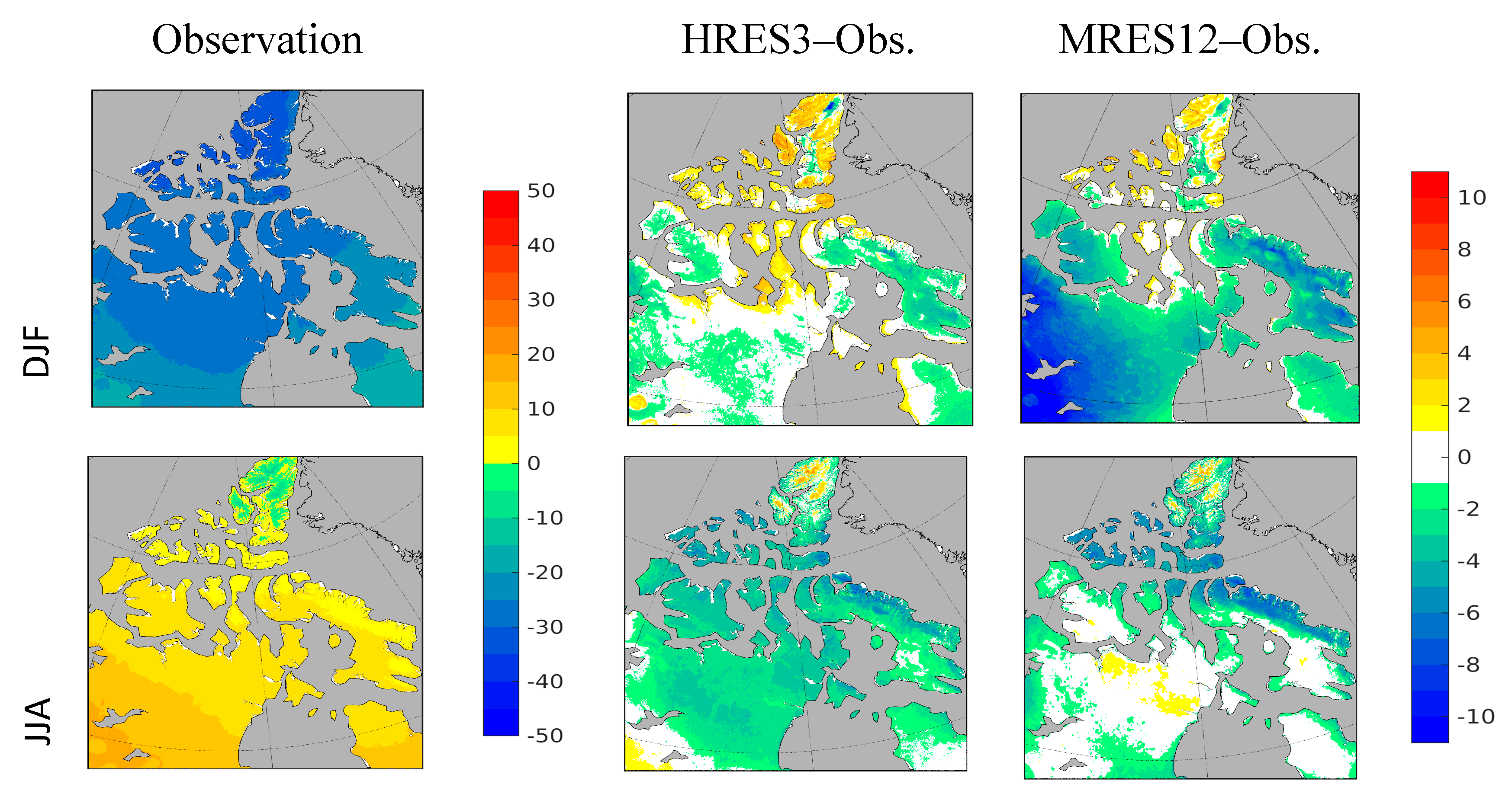
3. Validation of Seasonal Means and Annual Cycle

The observed seasonal mean climatology and the biases for the HRES3 and MRES12 simulations for summer and winter are presented in Figure 2. The prominent feature of the observed climatology of temperature is its large inter-seasonal variation. The mean winter temperature can reach below −30 °C and in summer it ranges from 10 °C to 15 °C for most of the domain. Both simulations exhibit cold biases for most of the domain except over the northern part during both seasons. For MRES12, a cold bias is noted over the southwestern part of the domain during winter season. This bias, however, is substantially reduced during summer with the maximum bias located over the Baffin islands. Though the seasonal mean temperature biases are lower in the HRES3 simulation, a clear improvement in temperature is noted only during the winter season as the bias in summer is generally visible throughout the domain. This implies that the high-resolution convection-permitting simulation is not always better in simulating seasonal mean temperature. The validation, however, should be taken cautiously as station observations are sparse over the Arctic (Figure 3, top left), which also deteriorates the Daymet quality.
Some of the benefits of convection-permitting simulations are illustrated in Figure 3, which shows the observed and simulated spatial distribution of winter and summer precipitation in HRES3 and MRES12. Observation shows relatively drier conditions towards the pole, particularly during the winter season. The maximum rainfall is experienced during summer; even during this season, the mean precipitation is generally less than 4 mm/day. The topographic influence is also noted along the Baffin Island coast. MRES12 produced a systematic dry bias during both seasons, particularly over the southern and western parts of the domain. The maximum dry bias in winter is found over the southwestern part of the domain and this is collocated with the maximum cold bias suggesting that these biases might be related to the use of non-cloudy/dry boundary layer scheme as opposed to the moist TKE scheme. This is because, in the dry scheme, diffusion is performed on the equivalent potential temperature and specific humidity with no effect on clouds. In contrast, the spatial distribution of precipitation is captured very well by HRES3 depicting higher values of precipitation over the southern and western part of the domain and lower values over the polar region and over the northwest. It has to be noted that the precipitation values plotted here are the sum of large-scale and convective precipitations, but a large fraction of the total precipitation (not shown) for this region is obtained from the large-scale precipitation (i.e., from the microphysics scheme) rather than from the convection parameterization.

Annual Cycle

The observed and simulated domain average annual cycle of temperature is shown in Figure 4 (right). The mean observed temperature ranges between −26 °C in January to 10 °C in July. Both simulations captured the annual cycle and the timing of peak correctly. The HRES3 reproduced the pattern well except during the summer months where it underestimates by about 2 °C, which is partly linked to the positive precipitation bias. The cold bias of MRES12 is apparent during the autumn and winter months Figure 4 (right), possibly due to the underestimation of precipitation. This cold and dry bias in the MRES12 simulation may be linked to the use of the dry boundary layer scheme. Figure 4 (left) compares the observed and simulated area averaged annual cycle of precipitation. Observation indicates that the lowest precipitation occurs during winter. Progressing towards summer, precipitation steadily increases to reach its maxima in August. Both model simulations captured these minima and maxima of the annual cycle correctly albeit with biases in magnitude. It is apparent from Figure 4 (left) that MRES12 substantially underestimates rainfall, particularity during summer months. HRES3, on the other hand, improved the simulation during these summer months when the rainfall is at its peak, even if it has a systematic positive bias.

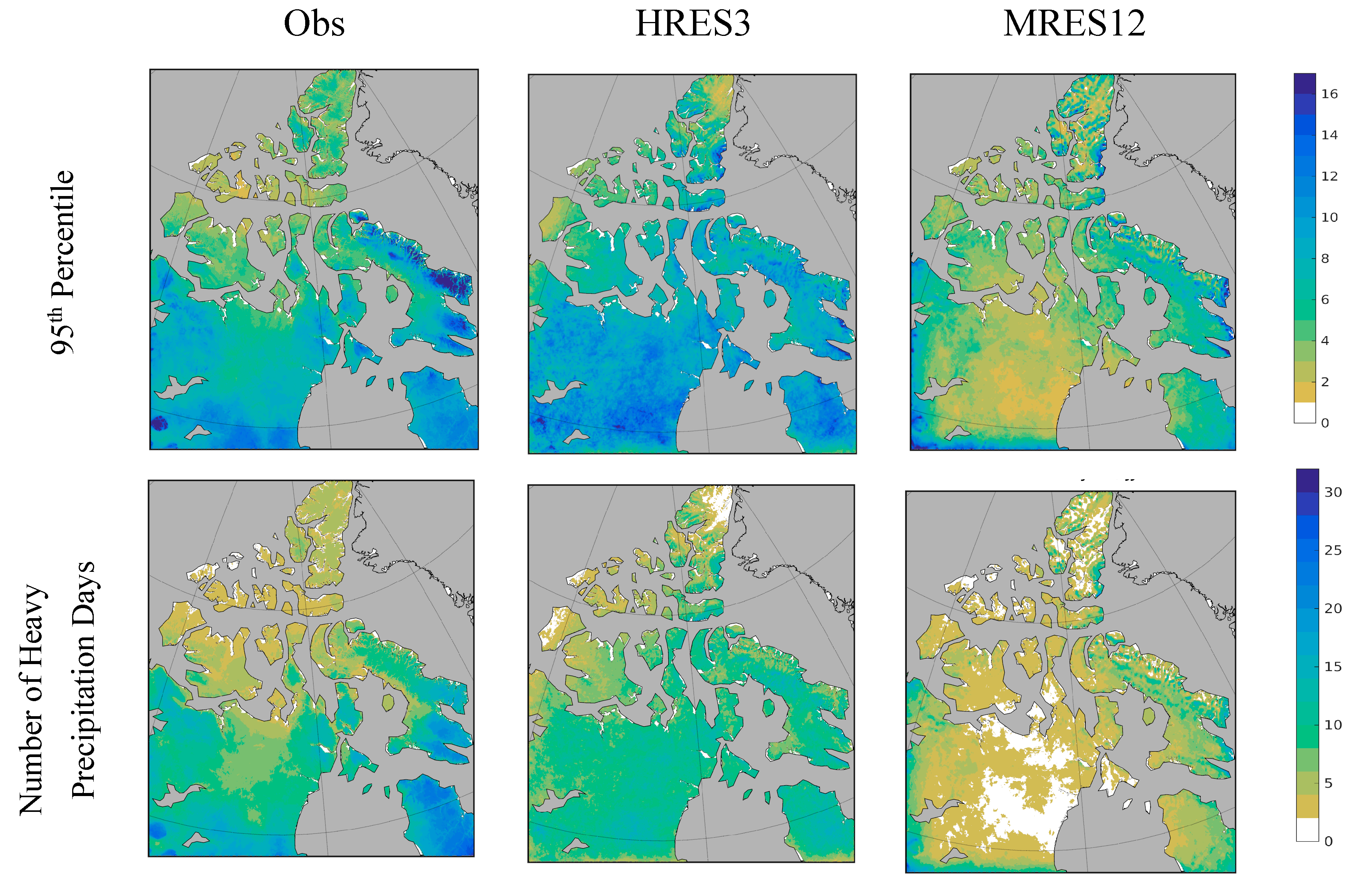
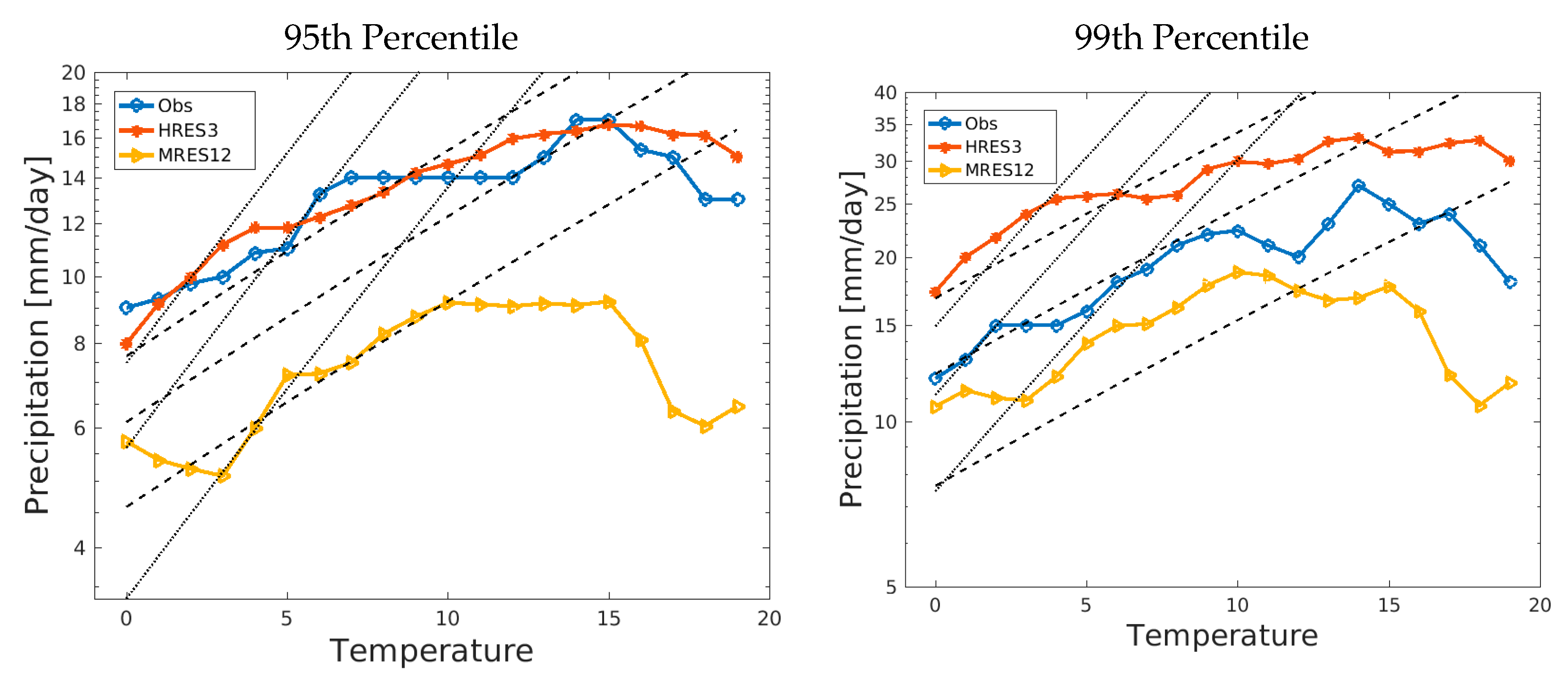
4. Daily Rainfall Extremes and P-T Relationship

The characteristics of precipitation extremes in the two simulations are assessed by computing the 95th percentile of daily summer precipitation and the frequency of heavy precipitation (≥5 mm/day) at every grid point as shown in Figure 5. Observation indicates that areas with higher intensity as well as the most frequent heavy rainfall events are collocated with regions receiving maximum seasonal precipitation namely northern Quebec, southern Nunavut, and eastern coastal areas of the Baffin Island. HRES3 shows similar broad patterns to those of Daymet and hence can be considered successful in reproducing the observed characteristics well, even if the percentage of heavy rainfall events is generally underestimated. Compared to HRES3 and Daymet, MRES12 substantially underestimates the intensity and frequency of extreme precipitation events consistent with its relatively low resolution. From the above analysis, there is a clear improvement in the model simulation in the frequency of occurrence of heavy precipitation when the model resolution is increased from 12 km to 3 km.
The frequency distribution of daily precipitation is illustrated in Figure 6. The figure generally shows that the frequency of precipitation events decrease with increasing intensity and this characteristic is reproduced by both simulations. It is also apparent that both simulations overestimate the frequency of precipitation less than ~2 mm/day and underestimate the frequency of precipitation events between 2–11 mm/day. MRES12 simulation, in particular, overestimates the frequency of light precipitation events and underestimates the medium and heavy precipitation events. Unlike the MRES12 simulation, the HRES3 simulations tend to capture the frequency of heavy precipitation events greater than 11 mm/day better, and generally exhibits consistently lower bias for all thresholds. This is consistent with the higher number of heavy rainfall events greater than the 95th percentile in the spatial distribution of extreme events discussed in the previous section.
Figure 7 shows the relationship between selected (95th and 99th) percentiles of the daily precipitation intensities (on logarithmic scale) against daily mean temperatures. From observation data, there is a clear increase of precipitation intensities with temperature until about 15 °C at a rate of approximately 7%/K, i.e., close to the C-C relation, but tends to decrease in precipitation intensity for temperature above 15 °C. Panthou et al. [18] also noted this decline of precipitation intensity at higher temperature for boreal forest regions of Canada and attribute it to the decrease of moisture at higher temperature. Both simulations more or less reproduced this observed characteristic, however MRES12 simulation show a sharp decline for temperatures beyond 15 °C. We also note that the scaling relationship is similar at both percentiles, however MRES12 underestimates at both percentile thresholds and HRES3 overestimates the precipitation extremes at the 99th percentile. The apparent difference in the slope of the scaling in MRES12 and HRES3 for higher temperature can also be attributed to the difference in the microphysics scheme used in the two simulations. As Singh and O’Gorman [53] indicated, the scaling of precipitation extremes with temperature is quite sensitive to the microphysics. This also implied that P-T scaling should be considered as one of the diagnostic metrics when selecting a suitable microphysics during model configuration.

5. Discussion and Conclusions

A convection-permitting simulation (HRES3) has been conducted at a horizontal resolution of 3 km over northern Canada for the 2008–2012 period. HRES3 is evaluated by comparing against coarse resolution (MRES12) simulation and a high-resolution (1 km × 1 km) observational dataset. It has to be noted that both HRES3 and MRES12 are driven by ERA5 reanalysis fields at the boundaries.
Comparison of the seasonal mean temperature indicated that both models exhibit cold biases in both seasons over most of the domain. HRES3 has a slight colder bias in summer and MRES has a stronger colder bias in winter. HRES3 improved the precipitation simulation by removing the dry bias in MRES12. In general, the precipitation simulated by HRES3 is slightly overestimated, which may partly be due to the uncertainties in the observations, as the observations over Arctic are sparse and located along the coast.
HRES3 is in better agreement with observations compared to MRES12 for depicting the precipitation spatial pattern. In general, precipitation is much more realistic in HRES3 than in the MRES12. This is also true for extreme precipitation, where the spatial and temporal patterns are better represented in HRES3. In MRES12, extreme precipitation is underestimated, while small-intensity precipitation (less than 2 mm/day) tends to be too persistent and wide spread.
Similarly, the intensity–frequency distribution of precipitation is better represented in the high-resolution simulation, particularly the frequency of rare but extreme precipitation events. Finally, we conclude that HRES3 produces better climate means and extremes compared to MRES12.
The scaling of heavy precipitation events with the ambient environmental temperature is also investigated for the region between 59° N to 65° N using observational data and the two simulations. The observed increase of heavy precipitation events with environmental temperature is found to follow close to the 7%/°C, which HRES3 captures well. MRES12 also reproduced this scaling fairly well for most of the temperature range, except for the lower and higher temperatures.
Several observational and modelling studies (e.g., [17,18]) have identified super CC scaling for short duration precipitation (i.e., sub daily and sub hourly). It would be interesting to assess how the MRES12 and HRES13 simulations represent the P-T scaling for these short-duration precipitation events.
This preliminary convection-permitting resolution simulation over northeast Canada provides useful insights and suggests the need for longer simulations than conducted here and more detailed analysis of other variables.

Author Contributions

Conceptualization, L.S. and G.T.D.; methodology, G.T.D.; validation, G.T.D.; formal analysis, G.T.D.; investigation, G.T.D. and L.S.; writing—original draft preparation, G.T.D.; writing—review and editing, G.T.D. and L.S.; visualization, G.T.D.; funding acquisition, L.S.

Funding

This research was funded by the Natural Sciences and Engineering Research Council (NSERC) of Canada.

Acknowledgments

This research was funded by the Natural Sciences and Engineering Research Council (NSERC) of Canada. ERA5 datasets are obtained from the European Centre for Medium-Range Weather Forecasts (ECMWF). GEM4.8.12 simulations considered in this study were performed on the supercomputer managed by Calcul Québec and Compute Canada. GEM-LAM v4.8.12 simulations can be obtained from the corresponding author.

Conflicts of Interest

The authors declare no conflict of interest.

References

  1. Johannessen, O.M.; Bengtsson, L.; Miles, M.W.; Kuzmina, S.I.; Semenov, V.A.; Alekseev, G.V.; Nagurnyi, A.P.; Zakharov, V.F.; Bobylev, L.P.; Pettersson, L.H.; et al. Arctic climate change: observed and modelled temperature and sea-ice variability. Tell. A Dyn. Meteorol. Oceanogr. 2004, 56, 328–341. [Google Scholar] [CrossRef] [Green Version]
  2. Jones, P.D.; New, M.; Parker, D.E.; Martin, S.; Rigor, I.G. Surface air temperature and its changes over the past 150 years. Rev. Geophys. 1999, 37, 173–199. [Google Scholar] [CrossRef]
  3. Serreze, M.C.; Walsh, J.E.; Iii, F.S.C.; Osterkamp, T.; Dyurgerov, M.; Romanovsky, V.; Oechel, W.C.; Morison, J.; Zhang, T.; Barry, R.G. Observational Evidence of Recent Change in the Northern High-Latitude Environment. Clim. Chang. 2000, 46, 159–207. [Google Scholar] [CrossRef]
  4. Chapman, W.L.; Walsh, J.E. Simulations of Arctic Temperature and Pressure by Global Coupled Models. J. Clim. 2007, 20, 609–632. [Google Scholar] [CrossRef]
  5. Francis, J.A.; Vavrus, S.J. Evidence linking Arctic amplification to extreme weather in mid-latitudes. Geophys. Res. Lett. 2012, 39, L0680. [Google Scholar] [CrossRef]
  6. Tang, Q.; Zhang, X.; Yang, X.; Francis, J.A. Cold winter extremes in northern continents linked to Arctic sea ice loss. Environ. Res. Lett. 2013, 8, 014036. [Google Scholar] [CrossRef]
  7. Vavrus, S.J. The Influence of Arctic Amplification on Mid-latitude Weather and Climate. Curr. Clim. Chang. Rep. 2018, 4, 238–249. [Google Scholar] [CrossRef]
  8. Vihma, T.; Pirazzini, R.; Fer, I.; Renfrew, I.A.; Sedlar, J.; Tjernstrom, M.; Lüpkes, C.; Nygard, T.; Notz, D.; Weiss, J.; et al. Advances in understanding and parameterization of small-scale physical processes in the marine Arctic climate system: A review. Atmos. Chem. Phys. 2014, 14, 9403–9450. [Google Scholar] [CrossRef]
  9. Mahlstein, I.; Knutti, R. Ocean Heat Transport as a Cause for Model Uncertainty in Projected Arctic Warming. J. Clim. 2011, 24, 1451–1460. [Google Scholar] [CrossRef]
  10. Taylor, C.M.; Birch, C.E.; Parker, D.J.; Dixon, N.; Guichard, F.; Nikulin, G.; Lister, G.M.S. Modeling soil moisture-precipitation feedback in the Sahel: Importance of spatial scale versus convective parameterization. Geophys. Res. Lett. 2013, 40, 6213–6218. [Google Scholar] [CrossRef]
  11. Prein, A.F.; Langhans, W.; Fosser, G.; Ferrone, A.; Ban, N.; Goergen, K.; Keller, M.; Tölle, M.; Gutjahr, O.; Feser, F.; et al. A review on regional convection-permitting climate modeling: Demonstrations, prospects, and challenges. Rev. Geophys. 2015, 53, 323–361. [Google Scholar] [CrossRef] [PubMed]
  12. Fosser, G.; Khodayar, S.; Berg, P. Benefit of convection permitting climate model simulations in the representation of convective precipitation. Clim. Dyn. 2015, 44, 45–60. [Google Scholar] [CrossRef]
  13. Allan, R.P.; Soden, B.J. Atmospheric Warming and the Amplification of Precipitation Extremes. Science 2008, 321, 1481–1484. [Google Scholar] [CrossRef] [PubMed] [Green Version]
  14. Kharin, V.V.; Zwiers, F.W.; Zhang, X.; Wehner, M. Changes in temperature and precipitation extremes in the CMIP5 ensemble. Clim. Chang. 2013, 119, 345–357. [Google Scholar] [CrossRef]
  15. O’Gorman, P.A.; Schneider, T. The physical basis for increases in precipitation extremes in simulations of 21st-century climate change. Proc. Natl. Acad. Sci. USA 2009, 106, 14773–14777. [Google Scholar] [CrossRef] [PubMed] [Green Version]
  16. Allen, M.R.; Ingram, W.J. Constraints on future changes in climate and the hydrologic cycle. Nature 2002, 419, 228–232. [Google Scholar] [CrossRef] [PubMed]
  17. Lenderink, G.; Van Meijgaard, E. Increase in hourly precipitation extremes beyond expectations from temperature changes. Nat. Geosci. 2008, 1, 511–514. [Google Scholar] [CrossRef]
  18. Panthou, G.; Mailhot, A.; Laurence, E.; Talbot, G. Relationship between surface temperature and extreme rainfalls: A multi-timescale and event-based analysis. J. Hydrometeorol. 2014, 15, 1999–2011. [Google Scholar] [CrossRef]
  19. Utsumi, N.; Seto, S.; Kanae, S.; Maeda, E.E.; Oki, T. Does higher surface temperature intensify extreme precipitation? Geophys. Res. Lett. 2011, 38, L16708. [Google Scholar] [CrossRef]
  20. Berg, P.; Moseley, C.; Haerter, J.O. Strong increase in convective precipitation in response to higher temperatures. Nat. Geosci. 2013, 6, 181–185. [Google Scholar] [CrossRef]
  21. Dai, A. Precipitation Characteristics in Eighteen Coupled Climate Models. J. Clim. 2006, 19, 4605–4630. [Google Scholar] [CrossRef] [Green Version]
  22. Wilcox, E.M.; Donner, L.J. The frequency of extreme rain events in satellite rain-rate estimates and an atmospheric general circulation model. J. Clim. 2007, 20, 53–69. [Google Scholar] [CrossRef]
  23. Ban, N.; Schmidli, J.; Schär, C. Evaluation of the convection-resolving regional climate modeling approach in decade-long simulations. J. Geophys. Res. Atmos. 2014, 119, 7889–7907. [Google Scholar] [CrossRef]
  24. Kendon, E.J.; Ban, N.; Roberts, N.M.; Fowler, H.J.; Roberts, M.J.; Chan, S.C.; Fosser, G.; Wilkinson, J.M.; Evans, J.P. Do Convection-Permitting Regional Climate Models Improve Projections of Future Precipitation Change? Bull. Am. Meteorol. Soc. 2017, 98, 79–93. [Google Scholar] [CrossRef]
  25. Stratton, R.A.; Senior, C.A.; Vosper, S.B.; Folwell, S.S.; Boutle, I.A.; Earnshaw, P.D.; Kendon, E.; Lock, A.P.; Malcolm, A.; Manners, J.; et al. A Pan-African Convection-Permitting Regional Climate Simulation with the Met Office Unified Model: CP4-Africa. J. Clim. 2018, 31, 3485–3508. [Google Scholar] [CrossRef]
  26. Ekström, M.; Gilleland, E. Assessing convection permitting resolutions of WRF for the purpose of water resource impact assessment and vulnerability work: A southeast Australian case study. Water Resour. Res. 2017, 53, 726–743. [Google Scholar] [CrossRef]
  27. Liu, C.; Ikeda, K.; Rasmussen, R.; Barlage, M.; Newman, A.J.; Prein, A.F.; Chen, F.; Chen, L.; Clark, M.; Dai, A.; et al. Continental-scale convection-permitting modeling of the current and future climate of North America. Clim. Dyn. 2017, 49, 71–95. [Google Scholar] [CrossRef]
  28. Prein, A.F.; Liu, C.; Ikeda, K.; Bullock, R.; Rasmussen, R.M.; Holland, G.J.; Clark, M. Simulating North American mesoscale convective systems with a convection-permitting climate model. Clim. Dyn. 2017, 1–16. [Google Scholar] [CrossRef]
  29. Côté, J.; Gravel, S.; Méthot, A.; Patoine, A.; Roch, M.; Staniforth, A. The operational CMC-MRB global environmental multiscale (GEM) model. Part I: Design considerations and formulation. Mon. Weather Rev. 1998, 126, 1373–1395. [Google Scholar] [CrossRef]
  30. Girard, C.; Plante, A.; Desgagné, M.; McTaggart-Cowan, R.; Côté, J.; Charron, M.; Gravel, S.; Lee, V.; Patoine, A.; Qaddouri, A.; et al. Staggered Vertical Discretization of the Canadian Environmental Multiscale (GEM) Model Using a Coordinate of the Log-Hydrostatic-Pressure Type. Mon. Weather Rev. 2014, 142, 1183–1196. [Google Scholar] [CrossRef]
  31. Hersbach, H.; Dee, D. ERA5 reanalysis is in production. ECMWF Newsl. 2016, 147, 5–6. [Google Scholar]
  32. Li, J.; Barker, H. A radiation algorithm with correlated-k distribution. Part I: Local thermal equilibrium. J. Atmos. Sci. 2005, 62, 286–309. [Google Scholar] [CrossRef]
  33. Benoit, R.; Côté, J.; Mailhot, J. Inclusion of a TKE boundary layer parameterization in the Canadian regional finite-element model. Mon. Weather Rev. 1989, 117, 1726–1750. [Google Scholar] [CrossRef]
  34. Delage, Y. Parameterising sub-grid scale vertical transport in atmospheric models under statically stable conditions. Bound.-Layer Meteorol. 1997, 82, 23–48. [Google Scholar] [CrossRef]
  35. Milbrandt, J.A.; Yau, M.K. A Multimoment Bulk Microphysics Parameterization. Part I: Analysis of the Role of the Spectral Shape Parameter. J. Atmos. Sci. 2005, 62, 3051–3064. [Google Scholar] [CrossRef] [Green Version]
  36. Sundqvist, H.; Berge, E.; Kristjánsson, J.E. Condensation and Cloud Parameterization Studies with a Mesoscale Numerical Weather Prediction Model. Mon. Weather Rev. 1989, 117, 1641–1657. [Google Scholar] [CrossRef]
  37. Mailhot, J.; Stéphane, B.; Robert, B.; Bernard, B.; Yves, D.; Luc, F.; Louis, G.; Claude, G.; André, T. Scientific Description of RPN Physics Library, Version 3.6; Recherche en Prévision Numérique, Service de l’environnement atmosphérique: Dorval, QB, Canda, 1998; Available online: http://www.cmc.ec.gc.ca/rpn (accessed on 2 October 2003).
  38. Verseghy, D. CLASS the Canadian Land Surface Scheme (Version 3.4); Technical Documentation (Version 1.1); Climate Research Division, Science and Technology Branch, Environment Canada: Toronto, ON, Canada, 2009. [Google Scholar]
  39. Verseghy, D.L.; McFarlane, N.A.; Lazare, M. Class—A Canadian land surface scheme for GCMS, II. Vegetation model and coupled runs. Int. J. Clim. 1993, 13, 347–370. [Google Scholar] [CrossRef]
  40. Verseghy, D.L. CLASS-A Canadian land surface scheme for GCMs. I. Soil model. Int. J. Climatol. 1991, 11, 111–133. [Google Scholar] [CrossRef]
  41. Martynov, A.; Sushama, L.; Laprise, R.; Winger, K.; Dugas, B. Interactive lakes in the Canadian Regional Climate Model, version 5: the role of lakes in the regional climate of North America. Tell. A Dyn. Meteorol. Oceanogr. 2012, 64, 16226. [Google Scholar] [CrossRef]
  42. Mironov, D.; Golosov, S.; Heise, E.; Kourzeneva, E.; Ritter, B.; Sceider, N.; Terzhevik, A. Flake-a lake model for environmental applications. In Proceedings of the 9th Workshop on Physical Processes in Natural Waters, Lancaster University, UK, September 2005; pp. 4–6. [Google Scholar]
  43. Kain, J.S.; Fritsch, J.M. The role of the convective? trigger function? in numerical forecasts of mesoscale convective systems. Theor. Appl. Clim. 1992, 49, 93–106. [Google Scholar] [CrossRef]
  44. Blackadar, A.K. The vertical distribution of wind and turbulent exchange in a neutral atmosphere. J. Geophys. Res. Space Phys. 1962, 67, 3095–3102. [Google Scholar] [CrossRef] [Green Version]
  45. Bougeault, P.; Lacarrere, P. Parameterization of Orography-Induced Turbulence in a Mesobeta—Scale Model. Mon. Weather Rev. 1989, 117, 1872–1890. [Google Scholar] [CrossRef]
  46. Bourgouin, P. A Method to Determine Precipitation Types. Weather Forecast 2000, 15, 583–592. [Google Scholar] [CrossRef]
  47. Bélair, S.; Mailhot, J.; Girard, C.; Vaillancourt, P. Boundary Layer and Shallow Cumulus Clouds in a Medium-Range Forecast of a Large-Scale Weather System. Mon. Weather Rev. 2005, 133, 1938–1960. [Google Scholar] [CrossRef]
  48. Gerard, L.; Piriou, J.-M.; Brožková, R.; Geleyn, J.-F.; Banciu, D. Cloud and Precipitation Parameterization in a Meso-Gamma-Scale Operational Weather Prediction Model. Mon. Weather Rev. 2009, 137, 3960–3977. [Google Scholar] [CrossRef]
  49. Hong, S.-Y.; Dudhia, J. Next-Generation Numerical Weather Prediction: Bridging Parameterization, Explicit Clouds, and Large Eddies. Bull. Am. Meteorol. Soc. 2012, 93, ES6–ES9. [Google Scholar] [CrossRef] [Green Version]
  50. Thornton, P.E.; Thornton, M.M.; Mayer, B.W.; Wilhelmi, N.; Wei, Y.; Devarakonda, R.; Cook, R.B. Daymet: Daily Surface Weather Data on a 1-km Grid for North America, Version 3 ORNL DAAC; Oak Ridge National Laboratory: Oak Ridge, TN, USA, 2017. [Google Scholar]
  51. Thornton, P.E.; Running, S.W.; White, M.A. Generating surfaces of daily meteorological variables over large regions of complex terrain. J. Hydrol. 1997, 190, 214–251. [Google Scholar] [CrossRef] [Green Version]
  52. Lenderink, G.; Van Meijgaard, E. Linking increases in hourly precipitation extremes to atmospheric temperature and moisture changes. Environ. Res. Lett. 2010, 5, 025208. [Google Scholar] [CrossRef]
  53. Singh, M.S.; O’Gorman, P.A. Influence of microphysics on the scaling of precipitation extremes with temperature. Geophys. Res. Lett. 2014, 41, 6037–6044. [Google Scholar] [CrossRef]
Figure 1. Topography (m) and free model domain for the HRES3 (red box) and MRES12 (blue box) simulations.
Atmosphere 10 00430 g001
Figure 2. Mean temperature climatology (°C, left column) and biases for high-resolution simulation (HRES3, middle column) and for low-resolution simulation (MRES12, right column) for winter (DJF, top row) and summer (JJA, bottom row) seasons.
Atmosphere 10 00430 g002
Figure 3. Seasonal mean precipitation (mm/day) for winter (top row) and summer (bottom row) obtained from observation (Daymet, left) and GEM4.8 simulations at high resolution (HRES3 middle column) and coarse resolution (MRES12, right column). The red dots in the top left panel represent the station distribution used in the Daymet dataset.
Atmosphere 10 00430 g003
Figure 4. Area-weighteddomain average annual cycle of precipitation (left) and temperature (right).
Atmosphere 10 00430 g004
Figure 5. Frequency (number of heavy precipitation days per summer) of extreme precipitation events (days) during JJA from observation (left), HRES3 (middle), and MRES12 (right) simulations.
Atmosphere 10 00430 g005
Figure 6. Empirical distribution of daily summer (JJA) precipitation as a function of precipitation thresholds.
Atmosphere 10 00430 g006
Figure 7. The 95th (left) and 99th (right) percentiles of daily precipitation intensity as a function of daily mean temperature for the region between 59° N and 65.5° N. Dashed and dotted lines correspond to the 7%/°C and 14%/°C, respectively. The Y-axis is plotted in logarithmic scale for convenience.
Atmosphere 10 00430 g007
Table 1. Summary of model configurations for HRES3 and MRES12 simulations.
Model PropertyHRES3MRES12
Horizontal resolution0.030.12
Number of grids(844 × 844)(220 × 220)
Vertical No. of levels5757
Time step for dynamics60 s300 s
Time step for Radiation15 min20 min
PBL shallow cloud/convNILCONRES [37]
MicrophysicsMPMY [35]ConSun [36]
ConvectionKain–Fritsch [43]Kain–Fritsch [43]
KFCdepth2000 m4000
KFCTRIG0.5 m/s0.15 m/s
KFCTIMEC1800 s2700 s
Planetary boundary layer cloud and convectionClef (non-cloudy boundary layer [33]Clef (non-cloudy boundary layer layer [33]
Mixing LengthBlac62 [44]Boujo [45]
Precipitation typeBourge [46]Extended Bourge (Bourge3d) [46]

