Simulations of Monsoon Intraseasonal Oscillation Using Climate Forecast System Version 2: Insight for Horizontal Resolution and Moist Processes Parameterization

Abstract

In the present study, we analyze the Climate Forecast System version 2 (CFSv2) model in three resolutions, T62, T126, and T382. We evaluated the performance of all three resolutions of CFSv2 in simulating the Monsoon Intraseasonal Oscillation (MISO) of the Indian summer monsoon (ISM) by analyzing a suite of dynamic and thermodynamic parameters. Results reveal a slower northward propagation of MISO in all models with the characteristic northwest–southeast tilted rain band missing over India. The anomalous moisture convergence and vorticity were collocated with the convection center instead of being northwards. This affected the northward propagation of MISO. The easterly shear to the north of the equator was better simulated by the coarser resolution models than CFS T382. The low level specific humidity showed improvement only in CFS T382 until ~15° N. The analyses of the vertical profiles of moisture and its relation to rainfall revealed that all CFSv2 resolutions had a lower level of moisture in the lower level (< 850 hPa) and a drier level above. This eventually hampered the growth of deep convection in the model. These model shortcomings indicate a possible need of improvement in moist process parameterization in the model in tune with the increase in resolution.

1. Introduction

India is predominantly an agricultural country; accordingly, the monsoon is of high socio-economic importance [1,2]. Monsoon rain, the primary source of water for agriculture, fills up reservoirs, recharges ground water, and brings up water level in rivers. Deficient summer monsoon rainfall [3,4], with an increase in heavy rainfall events [5], adversely affect the growth of crops [6]. This not only affects the economy but also the society at large. Thus, it is of utmost importance to have an accurate prediction of monsoon and its spatio-temporal variability. The contribution to monsoon rainfall comes from synoptic systems like depressions as well as the active and break cycles of monsoon [7]. In particular, the active-break cycles are governed by the northward propagating monsoon intraseasonal oscillations [8,9,10,11]. The prediction of these cycles is required as the frequency of occurrence of rain-bearing systems depend on it [12]. Although many advances have been made in this area, accuracy in forecasting the monsoon intraseasonal oscillations remains a challenge to the forecasters [13,14,15]. Multiple factors can contribute to the model performance in this aspect such as model physics, initial conditions, and resolution of the model grid. The simulation skill of Monsoon Intraseasonal Oscillation (MISO) varies amongst different models. Ref. [16] has explicitly shown that the CMIP5 models are able to capture the mean state of the Indian summer monsoon (ISM) broadly, but the spatial and temporal characteristics of MISO are not well represented. Only few of the 32 models analyzed showed a good pattern correlation and northward propagation of MISO.

The Climate Forecast System model (CFSv2) has shown good capability in the simulation of ISM. Previous studies have shown that CFS captures the mean precipitation by correctly identifying the centers of precipitation as well as the large scale monsoon circulation [17,18,19]. Although CFSv2 has certain drawbacks or systematic biases [20,21], such as the dry bias over Indian landmass, cold bias in Tropospheric Temperature (TT), cold bias in Sea Surface Temperature (SST), it has shown reasonable skill and robustness in seasonal and extended range prediction of ISM [22]. Ref. [23] explicitly shows that, although CFSv2 (T126) captures the mean rainfall over the Indian summer monsoon region, it does so with certain systematic biases. Dry bias over Indian landmass persists with a weak local Hadley circulation and an inaccurate ocean-atmosphere coupling (Bjerknes feedback) over the Equatorial Indian Ocean (EIO). Further, [24] highlights the biases in CFSv2 (T382). The distinctive findings in this study showed that, with an increase in horizontal resolution to T382, the simulated SST and tropospheric temperature is warmer than the observation; however, dry bias remains over the Indian landmass. Accordingly, a comprehensive comparison of performance of CFSv2 in simulating the intra-seasonal oscillations of ISM with different horizontal resolutions is required.

Ref. [25] provides a comparison of CFS at various horizontal resolutions (T62, T126 and T254) to assess their performance in predicting the Asian summer monsoon. They suggest that the higher model resolution predicted the magnitude and time of monsoon rainfall better than the lower resolutions. Ref. [26] examined CFSv2 for operational extended range prediction of MISO at T126 and T382 resolution. They showed that, although T382 had improved climatological biases, the forecast skill of MISO from T126 was similar to T382. They concluded that running a computationally intensive T382 operationally is not necessary for a real-time forecast and monitoring of MISO. Ref. [27] compared hindcast runs of CFSv2 at T126 and T382 for the simulation of ISM and its prediction skill. They found that the mean state and prediction skill of all India summer monsoon rainfall is better simulated in T382. In light of the performance of CFSv2, we studied its behavior in three resolutions, T62, T126, and T382. Here, we will focus on the simulation of MISO in these models. Previous studies have highlighted that rainfall in monsoon season is largely determined by the northward-propagating MISOs [11,13,14], which determine active and break spells in the season. Also, CFSv2 shows considerable skill in predicting it [28,29]. For the current work, we compare the simulation from three resolutions and we provide some insight on the behavior of moist process parameterization with increasing resolution and its impact on model fidelity in capturing characteristics and propagation of MISO.

2. Data and Methodology

The CFS version 2 was made operational at the National Centers for Environmental Prediction (NCEP) in 2011. This had major improvements over version 1, both in model and data assimilation system [30]. The atmospheric model is the Global Forecast System (GFS), which has a spectral triangular truncation at T126 and a finite differencing in the vertical with 64 sigma-pressure hybrid layers [31]. This is coupled with Modular Ocean Model 4 (MOM4) [32]. It also has an interactive three-layer sea ice model along with a four-layer Noah Land Surface Model [33]. For the present study, impact of model resolution was quantified by comparing the model data at different horizontal resolution with observation for various parameters. Only the horizontal resolution of model was changed to T62, T126, and T382. The model physics such as Simplified Arakawa Schubert (SAS) for convection, Zhao-Carr microphysics scheme, and the modified Rapid Radiative Transfer Model (RRTM), were kept same for all resolutions. In CFSv2, the sub-grid scale deep convection is parameterized by SAS, which is a mass flux-based scheme working on Arakawa-Schubert’s quasi-equilibrium assumption. The Zhao-Carr microphysics scheme takes into account grid scale precipitation. It incorporates both cloud ice and cloud water. These are represented by only one prognostic variable, i.e., the mixing ratio.

Daily data from a span of nine years from all the three model simulations was analyzed. Parameters such as precipitation, temperature, specific humidity, relative humidity, geopotential, vertical velocity, as well as U and V components of wind were taken for analysis from the model simulations. To compare model data with observation, daily data from various sources are taken. Tropical Rainfall Measuring Mission (TRMM) 3B42 [34] daily precipitation (0.25° × 0.25°) from 2004 to 2012 was used. Air temperature, specific humidity, relative humidity, U and V components of wind, geopotential and vertical velocity were taken from European Centre for Medium-Range Weather Forecasts (ECMWF) reanalysis (ERA) Interim daily [35] at 1° × 1° resolution for the same period as precipitation. Specific cloud liquid water was taken from ERA5 to calculate the precipitation efficiency.

To determine the MISO, a wavenumber-frequency analysis was performed on TRMM precipitation in meridional direction over the Indian region (15° S–30° N, 60° E–95° E) and in the zonal direction (10° S–10° N, global longitudes) for the eastward-propagating equatorial ISO. The spectra were calculated by performing a Fourier transform on May–October data, from which seasonal cycle had been removed. This provided the period of intraseasonal variability. The meridional spectra showed a temporal scale of 20–90 day period, which was used for filtering the data to analyze the northward propagation of MISO. Lanczos band-pass filter [36] of this period was applied on the data. This band-pass filtered data was then subjected to Empirical Orthogonal Function (EOF) analysis to select the MISO events. The first two modes of EOF featured the spatio-temporal characteristics of MISO. The first mode of EOF explained 61% variance and the second mode explained 25.6%. The strong MISO events were identified from the peaks in the time series of EOF₁ exceeding 1.0 and were termed as Day 0. Composite of these selected events was then prepared with a lag of ±15 days with respect to Day 0 for precipitation. Accordingly, Day 0 shows a composite of the strong MISO events or active spell of monsoon over the Indian region.

3. Results and Discussion

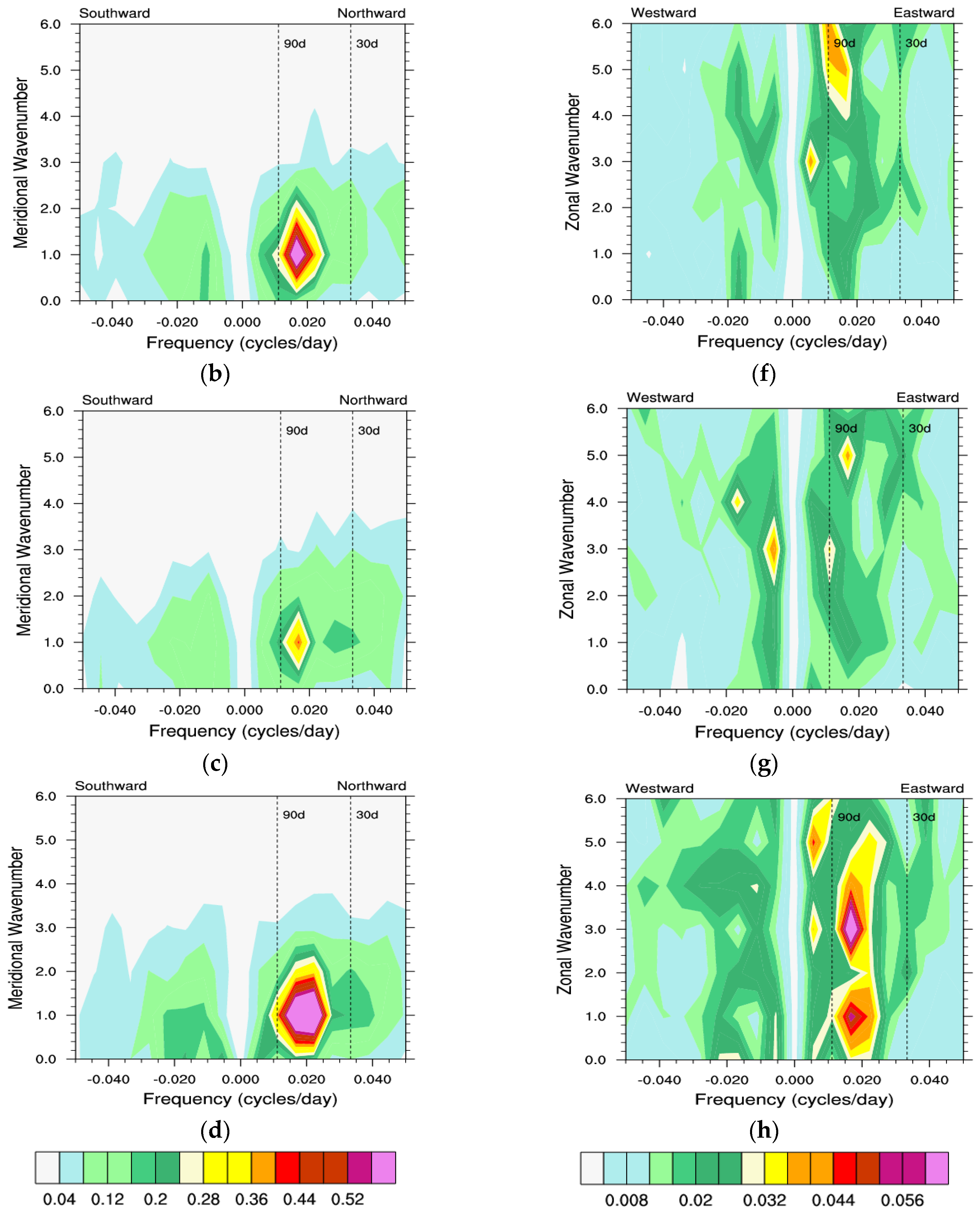
As the intraseasonal variability influences performance of the mean monsoon, fidelity of model in simulating or predicting the monsoon intraseasonal variability is of immense importance. To quantify the ability of the model, the north–south and east–west spectra of three resolutions of CFSv2, were analyzed for boreal summer precipitation anomaly, as seen in Figure 1.

The observed spectra in the meridional direction show maximum strength of power at wavenumber 1 and at a temporal scale of 40–50 days, as seen in Figure 1a. Further, there is another secondary peak power with periodicity of around 20 days [8]. Overall, a considerable strength in power is noted for 20–90 days. The spectra in zonal direction show a spatial scale of wavenumber 1 to 2 and temporal scale of 30–60 days with maximum power, as seen in Figure 1e. However, there is some significant power in the wave number 3 to 4.

As seen in Figure 1b, in the meridional direction, CFSv2 T62 shows maximum power at spatial scale of wavenumber 1 though with overestimation of power and with longer periodicity than the observation. With respect to eastward propagation, T62 does not show any peak power at wavenumber 1 and at periodicity of 40–50 days, as seen in Figure 1f. T126 also shows maximum power in the meridional direction at wavenumber 1 but with longer time period and with underestimation of power, as seen in Figure 1c. However, T126 shows a weak power in higher frequency, as is seen in the observation. T126 also shows a weak eastward propagation, as seen in Figure 1g. In meridional direction, T382 better simulates the spectra in terms of space and time but with an overestimation of power, as seen in in Figure 1d. T382 weakly captures the high frequency power. In the zonal spectra, T382 shows some improvement for eastward propagation although it produces an anomalous peak power at wavenumber 3 to 4, unlike the observation seen in Figure 1h. This shows that, with an increase in resolution, the model is able to capture the low frequency MISO, despite some overestimation in peak power.

As seen in Figure 2a, the composite of MISO events obtained through EOF analysis of observation data shows the organization and propagation of rainfall anomaly from the Indian Ocean to central India and then northwards from lag −15 to lag +15. The Lag 0 (strong MISO events) composite shows the rain band aligned over Central India. The graphical/grid center of this rain band gives the convection center used in further analysis. Although the model largely captures the anomalous rain bands associated with MISO, it shows that in all three resolutions the characteristic northwest-southeast tilt is missing and contrary to the observation, a zonally oriented rain band is seen, as seen in in Figure 2b–d.

To further quantify the composites we calculated the pattern correlation between observation and all models for different lag time, as seen in Figure 3.

The models show a similar correlation for all time lags; however, Lag −10 shows a negative correlation when compared with other lags. Upon careful observation of Lag −10 composite in Figure 2a–d, two branches of positive anomaly and one of the branch moves toward the Indian west coast and the other branch of positive anomaly shows a large scale organization near the equatorial Indian Ocean to the Bay of Bengal, with the northern Bay of Bengal showing a negative anomaly. T126 shows the positive anomaly over the Indian west coast on 10 days lag very clearly; in contrast, T62 and T382 shows the positive anomaly away from the coast, as seen in Figure 2b–d. However, all three models poorly simulate the organized positive anomaly over the equatorial Indian Ocean and the Bay of Bengal; they also miss the negative anomaly over the northern Bay of Bengal. This appears to be the reason behind abrupt low correlation for −10 days lag.

The model largely captures the features of MISO but with some discrepancies. Moisture and wind components were analyzed because these fields play a key role in maintaining and propagating the MISO northward. As seen in Figure 2, similar lag composites were prepared for the moisture convergence and vorticity to understand the vertical structure and its propagation during MISO events. Figure 4a shows the composite of anomalous vorticity based on ERA reanalysis dataset for strong MISO events from lag −15 to +15, with respect to the convection center. The center of maximum convection seen in Lag 0 of Figure 2a was chosen as the convection center. Thus, moving to the right (left) of 0 on X axis of Figure 4a implies north (south) of convection center. The anomalous vorticity in Figure 4a shows a barotropic structure for Lag 0, with the positive vorticity centered at about 300 km north of convection center. The propagation of the anomalous positive vorticity northward is evident from Lag −15 to Lag +15. In case of T62, as seen in Figure 4b, negative vorticity is seen in the upper levels to the north of the convection center. Accordingly, the barotropic structure is missing and appears to be tilted southwards for all Lags. T126, as seen in Figure 4c, and T382, as seen in Figure 4d, simulations show a better vertical structure, with some barotropicity by reducing the southward tilt; the negative vorticity in the upper levels is evident in both higher resolutions in comparison with T62.

Further, as seen in Figure 5a, at Lag −15, a positive anomaly of moisture convergence is present in the lower levels to the south of convection center and a negative anomaly to the north of convection center. In the subsequent Lag −10, −5, 0, and 5, the negative anomaly to the north of convection center shows a gradual transition to a positive anomaly. This is a key feature responsible for MISO propagation, as shown in previous studies [37,38]. Unlike the analysis based on ERA seen in Figure 5a, T62 poorly captures the positive anomaly to the south of convection center at Lag −15; however, it shows a positive anomaly at Lag −5 and Lag 0, as seen in Figure 5b. Beyond Lag 0, T62 does not show the low level moisture convergence to the north of convection center. T62 fails to reproduce the realistic transition of low level moisture convergence in the lower levels (within 850 hPa), suggesting a possible model shortcoming in representing one of the key process, i.e., the moisture convergence associated with MISO. As seen in Figure 5c, T126 shows a weak positive anomaly at Lag −15; however, at Lag −10, it fails to show realistic moisture convergence in the lower levels (absence of positive anomaly to the south of the convection center). In contrast, at Lag −5 and Lag 0, T126 shows a reasonable positive anomaly of moisture convergence to the north of convection center, but, at Lag +5, it shows the moisture convergence between 700 and 850 hPa, unlike the ERA. T382 shows an improved moisture convergence at Lag −15 to the south of convection center, as seen in Figure 5d. However, at Lag −10, it underestimates the lower level moisture convergence, but at Lag −5, Lag 0, and Lag +5, it shows a positive moisture convergence in the lower levels better than T62 and T126.

The above analysis suggests that lower level moisture convergence anomalies associated with MISO are simulated better with T382 when compared with T62 and T126.

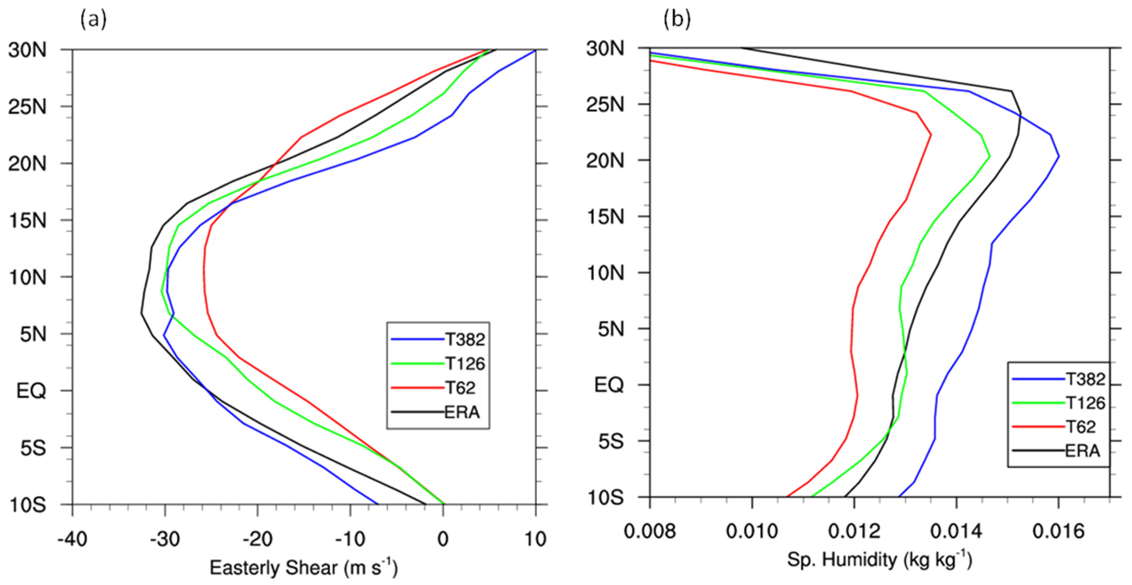
In an exploration of this topic, [37] showed that the vertical shear generates barotropic vorticity, which, in turn, shifts the moisture convergence to the north of the convection center and is responsible for the northward propagation of MISO. Hence, the meridional structure of easterly wind shear (the difference between zonal wind at 200 hPa and 850 hPa) and low level-specific humidity (averaged between 1000–850 hPa) during MISO events is plotted by averaging between 65°–95° E. As seen in Figure 6a, the easterly shear (U200-U850) simulated by the models is weaker than the reanalysis except to the south of equator for T382 and north of 20° N for T62. The peak in easterly shear found between 5° N and 15° N in the reanalysis is underestimated in all three models. In Figure 6b, the low level moisture is better simulated by T126, whereas T62 underestimates and T382 overestimates up to ~20° N when compared with the ERA reanalysis. There is a southward shift in the peak obtained in all models with respect to ERA.

This indicates that the models underestimate the northward extent of the low level moisture and easterly shear, both of which are not conducive for the MISO propagation.

Moist Static Energy (MSE) is a measure of moist instability. A high MSE indicates high moist instability in the atmosphere and could favor the occurrence of deep convection. To quantify the relationship between moist instability and precipitation in the model, joint distribution of rainfall and vertically integrated MSE over 15° S–30° N, 60° E–95° E for the MISO events is shown in Figure 7.

The shaded contours represent the joint distribution of rainfall and MSE for observation. It suggests that there is no deterministic relation between MSE and rainfall as there are events (counts) when higher MSE produces lighter rain as well as counts (events) of higher rain with high MSE. In Figure 7a–c, the contours are for T62, T126, and T382, respectively. T126 better coincides with the observation whereas T62 shows a left-skewed distribution, suggesting that, with lower values of MSE, it is producing rainfall as much as the observation. In the case of T382, the distribution is skewed to the right, indicating that it requires higher MSE to produce rainfall as per the observation. For T382, we also noticed that the model did not produce higher rainfall categories. Analyses indicate that, with the increase of resolution, the model generates more moist instability but the count of heavier rain reduces.

Another diagnostic metric correlating precipitation and moist processes was performed by [39,40]. Here we plotted the vertical structure of relative humidity with respect to precipitation rate for the ISM region and for the MISO events. A similar analysis was done with upward moisture flux (ωq/g) with respect to precipitation to further diagnose the vertical moisture profile. These analyses demonstrated the cause of absence of deep convection in this section. In Figure 8 and Figure 9, we show the vertical column of relative humidity and upward moisture flux (ωq/g) corresponding to a particular range of precipitation rate for the MISO events, respectively.

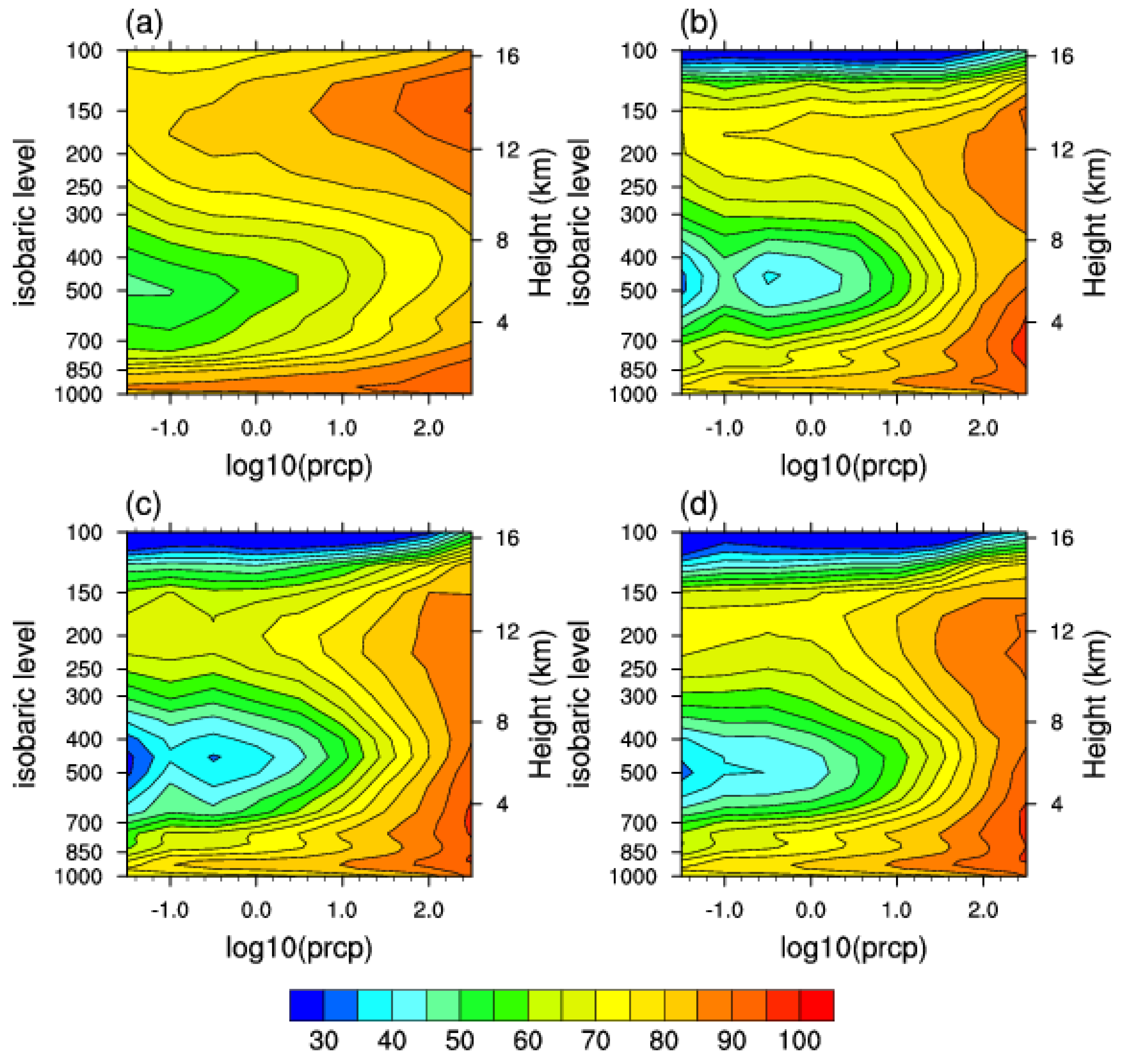
The TRMM and ERA based analyses (observation) shows that, for lower rain rate, there is a high relative humidity confined within the lower levels (within 850 hPa~1.5 km), as seen in Figure 8a. This lower level moistening gradually increases for higher rain rates. High precipitation occurs when the whole tropospheric column becomes sufficiently moist with >75% humidity. In Figure 8b–d, the models show a dry area of <50% humidity from 700 hPa to 300 hPa for lower rain categories. This dry area is absent in the observation and it shows >50% humidity in the layer (700–300 hPa). The models in all resolutions (T62, T126, and T382) show a similar distribution with deep moist layer associated with the higher rain rates and a drier level in the middle troposphere (700–300 hPa) associated with the lighter and moderate rain rate. This indicates that all three versions of the model have similar representations of moist process parameterization; accordingly, the bias appears much similar with the rain rates associated with the MISO. After documenting the shortcomings of all the models in reproducing the vertical distribution of moisture with different rain rates, we intend to analyze the upward moisture flux for the MISOs.

As seen in Figure 9a, there is an upward moisture flux present for all the rain rates from lighter to heavier rates. Shallow downward flux can be seen only for very low rain rate category. In the models seen in Figure 9b–d, unlike the observation, the downward flux of moisture dominates throughout the column for lower rainfall. More subsidence is visible in the low to moderate rain rate and the gradual transition (from low to high values) of flux is missing. In concurrence with relative humidity structure, the upward moisture flux also shows a deeper column for higher rain rates in all models. Figure 8 and Figure 9 demonstrate the possible shortcoming of the role of moisture and its vertical flux on different rainfall categories associated with MISO. The improper moist process of the models is further clarified in Figure 10 which shows the vertical (subgrid scale) turbulent flux of moisture $(\overline{{\mathsf{\omega }}^{\prime }{\mathrm{q}}^{\prime }})$.

Analysis of vertical turbulent flux (Figure 10) of moisture $(\overline{{\mathsf{\omega }}^{\prime }{\mathrm{q}}^{\prime }})$ is also assessed for MISO events. Here ω′ and q′ is calculated by subtracting ω and q at each grid point from its grid average at a particular level. It is then averaged for the MISO events and over the ISM region (15° S–30° N, 60° E–95° E). The ERA analysis (black) shows updrafts or upward flux of moisture even up to 400 hPa and attains a peak at about 800 hPa, whereas all the models attain a peak value at lower pressure level of 900 hPa with no significant difference among the models. The models simulate weak updrafts only upto about 750 hPa, indicating that the transport of moisture is restricted to a much lower level than the observation. Such weak vertical moisture turbulent flux in the models further demonstrates the lack of transport of moisture in the upper levels affecting the deep convection in the models.

To quantify the process of cloud condensation and rainfall generation, the precipitation efficiency “f” is calculated for all resolutions. It is defined as the ratio of precipitation rate accumulated for the MISO events and over the ISM region (15° S–30° N, 60° E–95° E) to the total grid box cloud water path for the same events [41]. The precipitation efficiency “f” has units of days⁻¹ and it implies an inverse timescale for the conversion of cloud water path to precipitation. A larger value of “f” implies a shorter timescale for the conversion process and vice versa. Precipitation efficiency of a model depicts its capability of converting cloud water to precipitation. It quantifies the role of microphysics in production of precipitation. Figure 11 shows the precipitation efficiency of the models with respect to rainfall bins.

The models show similar efficiency for rainfall up to 64.4 mm/day. But for heavier rainfall, T382 shows least efficiency when compared with the other two resolutions. Although the models match the observation for rainfall up to 15.5 mm/day, the precipitation efficiency of the models are significantly lower for higher categories of rainfall. Lower values of “f” signifies that the model takes more time for conversion from cloud water path to rain of respective category which eventually makes its efficiency lower. This analysis indicates the need for better moist process (cloud and convection) parameterization suitable for high resolution models.

Another important factor associated with convection is the heating in the atmospheric column. To show this, the apparent heat source (Q1) is calculated following [42], as seen in Figure 12. Q1 is calculated for MISO events for the region 12° S–30° N, 65° E–95° E.

The models underestimate the heating in the whole vertical column of troposphere when compared with reanalysis, as seen in Figure 12. Among the resolutions, T382 shows the least amount of heating. At lower levels (below the boundary layer), T62 and T126 perform identically but above 800 hPa, both the resolutions show higher heating than T382 and much weaker heating than ERA reanalysis. Such improper heating distribution throughout the atmospheric column is consistent with earlier analyses suggesting weaker deep convection in the models irrespective of increase in resolutions.

4. Conclusions

We have analyzed three resolutions, T62, T126, and T382 of CFSv2 with respect to observation/reanalysis in the present study to bring out the deficiency in the moist convective parameterization with increasing resolution. To accomplish this, we chose to analyze the simulation of MISO, focusing on its characteristics and propagation. The wavenumber-frequency spectra showed a longer time period in all models and a lack of eastward propagation. However, T382 better captured the spatial and temporal scale than its counterparts. The composite of MISO events obtained from EOF analysis of the filtered data shows northward propagation but with a slower speed and with the characteristic northwest-southeast tilt missing. The slower propagation appears to be affected by the weak easterly shear as well as by the improper representation of vorticity and low level moisture convergence.

The analyses of MSE and rain rate suggest that the heavier rain rate counts are lesser in the high resolution model (T382) despite the model showing more MSE. This analysis further prompts us to investigate the distribution of moisture content in the vertical and its upward flux. Both vertical distribution of moisture with different rain rates of MISO and the upward moisture flux associated with the rain rates of MISO elucidate the shortcomings of all three models to realistically represent the lower level moist process. The moist process deficiency appears to be similar irrespective of the resolution. This indicates that the advantage that one would achieve by increasing resolution is lost due to improper moist process parameterization, particularly in the lower levels. The improper upward moisture flux at the lower level could possibly be one of the reasons behind a lack of deep convection in all the resolutions of CFSv2 model.

Although higher resolution of model showed improvement, enhancing the model physics suitable for higher resolution is essential. We also computed the precipitation efficiency for respective rainfall categories; for all three models T382 showed a lesser precipitation efficiency for higher rainfall, implying the model takes a longer time in the conversion of cloud water path to precipitation. The fundamental property of higher vertical velocity, i.e., updraft (Figure not shown) and heating throughout the vertical column, which is required for proper representation of convection, was found to be very weak in all resolutions of the model. This leads to unrealistic convection (lack of deep convection) and higher occurrence of lighter rainfall (Figure not shown). The CFSv2 T382 is the current operational model for seasonal forecast of Indian summer monsoon, and diagnostics that emphasize the key moist process associated with the MISO could be helpful for further model development.