Abstract
The atmospheric background CO2 concentration is a key quantity for the analysis and evaluation of the ongoing climate change. Long-term CO2 observations have been carried out at the high Plateau Rosa mountain station, in the north-western Alps since 1989. The complete time series covers thirty years, and it is suitable for climatological analysis. The continuous CO2 measurements, collected since 1993, were selected, by means of a BaDS (Background Data Selection) filter, to obtain the hourly background data. The monthly background data series was analysed in order to individuate the parameters that characterise the seasonal cycle and the long-term trend. The growth rate was found to be 2.05 ± 0.03 ppm/year, which is in agreement with the global trend. The increased background CO2 concentration at the Plateau Rosa site is the consequence of global anthropic emissions, whereas the natural variability of the climatic system taken from the SOI (South Oscillation Index) and MEI (Multivariate ENSO Index) signals was detected in the inter-annual changes of the Plateau Rosa growth rate.
1. Introduction
The growth of the atmospheric concentration levels of greenhouse gases in the Industrial Age is considered the major cause of the observed warming of the Earth’s surface [1]. Carbon dioxide (CO2) is the primary gas that is contributing to the enhanced greenhouse effect, and the largest contribution to total radiative forcing is caused by the increase in the atmospheric concentration of this atmospheric component [1,2]. For this reason, the CO2 concentration in the atmosphere is considered a key quantity to study and understand the global greenhouse effect and the ongoing climate change, and it is constantly monitored at several locations around the world, and in particular at remote sites [3,4,5,6]. These locations are at a great distance from significant anthropogenic sources of air pollutants, so that the CO2 background concentration measurements are poorly influenced by local sources or transport. The long-term observations of the CO2 background atmospheric concentration are of fundamental importance to investigating ongoing climate change and represent a useful tool to evaluate the success of mitigation activities against climate change.
The CO2 concentration has been measured at the Plateau Rosa site, located in the westerly Italian Alps near Mt. Cervino in Italy, at the altitude of 3480 m a.s.l., since 1989 (and continuously since 1993). The geographical position of the station, that is, at a high altitude and far from urbanised and industrialised zones, allows representative measurements of the atmospheric CO2, CH4 (methane) and O3 (ozone) background values to be obtained frequently [7].
Several analyses have been carried out since the beginning of the CO2 monitoring activity. In the first studies about the CO2 concentration time series at Plateau Rosa, the daily concentrations were shown for the 1989–1992 period [8] and the connections between the measured CO2 values, which were available at that time, were analysed, together with the meteorological circulation patterns [8,9]. The deterministic backward trajectories were computed every 6 h and a cluster analysis was used for this purpose. Later on, the monthly mean data for the 1989–1999 period were shown by Ferrarese et al., (2002) [10], who investigated the source and sink areas over Europe and the Boreal Atlantic Ocean by means of a source-receptor model [11] on the basis of backward trajectories starting from at Plateau Rosa. The monthly data averages for the 1989–2001period were published by Apadula et al. (2003) [12], who computed a growth rate of 1.52 ppm/year. The column concentration fields for 1996–1997 were computed using the same source-receptor model, the backward trajectories and the CO2 concentrations from three monitoring sites at high altitudes in Europe: Plateau Rosa, Zugspitze and Monte Cimone. The 20-year-long monthly data (1993–2013) were presented by Ferrarese at al. (2015) [13], who evaluated the growth-rate of that period (1.98 ± 0.04 ppm/year). A detailed analysis of atmospheric circulation was performed using a regional meteorological model to investigate the source areas of the highest concentration event in the complete series available at that time.
Moreover, subsets of CO2 concentration data have been used in studies on a global scale and a regional scale [14,15,16].
The CO2 concentration series is now thirty years long, which is a significant period of time from a climatic point of view, because the climate is frequently defined as covering a 30-year time period. The background Plateau Rosa CO2 monthly concentration data series is here presented and analysed, the main distinctive parameters are pointed out and the method used to obtain the background data is illustrated.
The Plateau Rosa station (Section 2) is described in this paper, together with its monitoring instrumentation (Section 3). The filtering method used to select the background data is detailed (Section 4) and the main features of the CO2 monthly concentration time series are discussed (Section 5). The inter-annual variability is analysed in Section 6, and the conclusions are summarised in Section 7.
2. Plateau Rosa Monitoring Station
The Plateau Rosa monitoring station (Global Atmosphere Watch (GAW) Identification Code: PRS) is located in the north-western Alps, in the Italian Aosta Valley region, in the municipality of Valtournenche, near Mt. Cervino. The PRS station (Figure 1) is located inside the Testa Grigia Laboratory, which belongs to the CNR (Italian National Research Council).
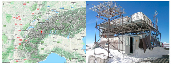
Figure 1.
Geographical position of PRS (north-western Italian Alps, geographical coordinates: 45.93436° N, 7.70778° E, 3480 m a.s.l.) (a), picture of the PRS (b).
The station (45.93436° N, 7.70778° E) was installed at an altitude of 3480 m a.s.l., upon a large snow-clad mountain plateau far from urban and polluted zones. PRS is one of the highest monitoring stations of the World Meteorological Organization GAW Programme [7]. Owing to its high altitude and position, it is very often located above the planetary boundary layer, and is thus suitable for the background measurement of greenhouse gases.
The measurement of the most important greenhouse gases (excluding water vapour), such as CO2, CH4, and O3, is carried out at the PRS station by RSE (Ricerca sul Sistema Energetico—Italy), and a neighbouring meteorological station, also managed by RSE, was installed to support the greenhouse gas measurements, by collecting, in real time, air temperature, relative humidity, pressure and wind (speed and direction) data.
Since these measurements should not be influenced by local sources, the PRS station is equipped with an electrical heating system and does not use any fossil fuel. During the skiing season, diesel-operated snowmobiles are sometimes used to maintain appropriate conditions for the skiing activity, but they operate at lower altitudes, and thus do not influence the measurements. A refuge and a cable car are located in the vicinity of the measuring station; both only operate during daylight hours and are open for about eight months a year. A meteorological station, managed by the Italian Meteorological Service (WMO code: 16052), is located at a horizontal distance of about one hundred meters from the PRS.
The wind speeds are generally greater than 4 m s−1, and thereby reduce any eventual impacts of local sources. An analysis of the intensity and direction of the winds gathered in the 1971–2008 period at the Italian Meteorological Service station showed that calm conditions (lower wind speeds than 1 m s−1) occurred during about 17% of the measurements, while the prevailing winds came from North East (about 25% of the events). The wind rose pertaining to one entire year, with a data coverage of about 98%, as measured at the RSE meteorological station, is shown as an example in Figure 2. A wind speed of less than 1 m s−1 occurred in 5% of the observations, while it was higher than 4 m s−1 in about 60% of the measurements and higher than 6 m s−1 in more than 40% of the measurements.
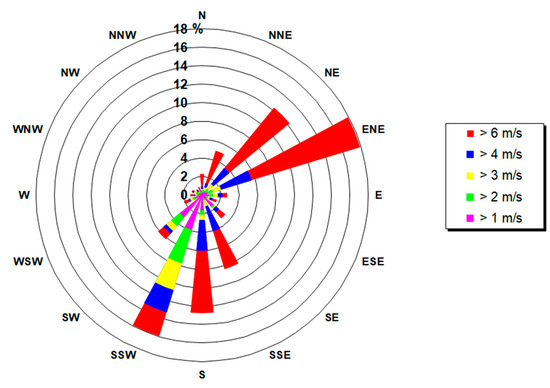
Figure 2.
Wind rose at PRS for the year 2012 (RSE meteorological station).
The climate at the Plateau Rosa station is typical of a continental alpine location, with relatively large diurnal and seasonal temperature variations, frequent atmospheric pressure variations and strong winds. The climatological mean values (for the 1961–1990 period) of the maximum and minimum temperatures measured at the Italian Meteorological Service station (PRS site) are shown in Figure 3 [17].
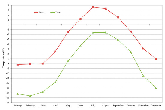
Figure 3.
Mean values of the maximum (Tx-m) and minimum (Tn-m) temperatures for the 1961–1990 period [17].
3. CO2 Measurement Instrumentation
The measurements of CO2 at PRS began in April 1989, with the valuable collaboration of the Italian Meteorological Service personnel working at the Monte Cimone monitoring station, who carried out the analyses of the air samples collected at the PRS station by means of a non-dispersive infrared (NDIR) analyser (ULTRAMAT 3E). The air samples were taken every two weeks, using a couple of electropolished stainless steel flasks, at different hours of the day (usually at 9:00, 11:00, 13:00, and 15:00, local time). All the samples were then transferred to the Monte Cimone laboratory where they were then analysed.
In March 1993, PRS set up its own measurement system, which involved the installation of an NDIR ULTRAMAT 5E analyser, manufactured by SIEMENS. The inlet height of the instrument is about 9 m above ground. Both types of measurements (continuous and flask measures) were carried out for about 4 years, until December 1997, and a good agreement between the two types of measurements was observed.
The analyser system is calibrated regularly. The calibration procedure consists of three different steps: the first one regards the measurement of the air by means of two working gas standards (every six hours); the second one involves checking the secondary standards (every 72 h); the third one makes use of five referenced NOAA (National Oceanic and Atmospheric Administration) primary gas standards (referenced scale WMO X2007 [18]), and this is performed at least once a year. This type of approach is based on the work of Komhyr et al. (1989) [19] and Cundari et al. (1995) [20]. The two working gas standards are compared every 72 h with four well-calibrated secondary station standard gases in order to obtain a better determination of their CO2 concentrations and any possible drifts in the concentration with time (measurement scheme shown in Figure 4). The working and secondary standards were acquired from S.I.A.D. (Società Italiana Acetilene e Derivati) and the primary standards were purchased from NOAA ESRL/GMD (National Oceanic and Atmospheric Administration—Earth System Research Laboratory/Global Monitoring Division). The working and secondary standards, before being utilised, are referenced to the primary standards in order to determine the values with respect to the WMO X2007 scale. Finally, the current primary standards were supplied by the ICOS (Integrated Carbon Observation System) project [6]. The NOAA primary standard concentrations range from 369.58 to 404.64 ppm and the ICOS concentrations range from 379.194 to 449.890 ppm.
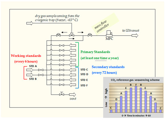
Figure 4.
Measurement scheme (the CO2 reference gas sequencing scheme is similar to the one proposed by Komhyr et al. [19]).
The uncertainty of the measurements was estimated as 0.07 ppm on the basis of various replicated measurements of some working standards with different concentration values. The uncertainty was basically assumed to be equal to the standard deviation assigned to the average value of the differences between the certified value of the standard and that measured by the instrument (the measurements were related to a period of 9 months and the working standards were measured every six hours).
All the gases are dried, prior to being introduced into the analyser, by passing them through a glass water vapour trap, immersed in a cold alcohol bath maintained at −65 °C by means of a freezer. This approach is particularly important to express the CO2 concentration in dry air. The atmospheric CO2 concentration, with reference to the WMO X2007 international mole fraction scale, is expressed in ppm, i.e., in μmoles/mol of dry air. The native data frequency is 0.2 Hz. The measured data was averaged every 30 min until 2007, and then every 60 min in order to be consistent with international measurement standards. The corresponding standard deviations have been computed.
A PICARRO 2301 analyser, with all the necessary accessories for the real-time measurement of CO2, CH4 and H2O, was installed in May 2018 and it was made operational, according to ICOS guidelines [6,21], in September 2018. Therefore, since that date, the measurement of the CO2 concentration has been carried out with both monitoring systems (PICARRO and ULTRAMAT), and the homogeneity of the measurements is tested by measuring the concentration of the primary reference standard mixtures with both instruments. The comparison of the measurements has shown a high comparability, as the maximum obtained differences are lower than 0.1 ppm, and are thus compatible with the above-mentioned measurement standard uncertainty.
The standard calibration mixtures adopted for the new measurement system (PICARRO) are provided within the ICOS project. The used measurement scheme is quite similar to that required by ICOS, to which the Plateau Rosa monitoring station has to comply [21]. The timing of the calibration verification has changed significantly, as result of the stability of the new analyser, compared to the measurement system carried out using the ULTRAMAT analyser. In addition to the four reference primary standards, a Short-Term Target Gas (STTG), with one measurement every 24 h, and a Long-Term Target Gas (LTTG), with one measurement every 30 days, were introduced to check the stability of the measurement in the short and long term. The duration of the measurement of each standard is 15 min, and the calculation of the average value is carried out without considering the first three minutes of the measurements. In agreement with ICOS ATC (Atmosphere Thematic Centre), we are planning to modify the plant by increasing the STTG measurement frequency and making the plant more like the one indicated by Laurent [21].
Finally, it is important to point out that, since all measurements in the global monitoring network must be comparable with each other, they refer to a single measurement scale. For this reason, various and systematically inter-comparison campaigns have been conducted and managed by NOAA on behalf of WMO/GAW in the context of several European projects. The CO2 inter-comparability target for WMO is 0.1 ppm.
The CO2 data collected at the Plateau Rosa station are available at WDCGG (World Data Centre for Greenhouse Gases) and in ObsPack (Observation Package) [5,22].
4. Background Data Selection
The identification of atmospheric trace species measurements, which are representative of well-mixed background air masses, thus unaffected by local conditions, is particularly important to monitor atmospheric composition variations at background sites, and to document the long-term CO2 changes in the atmosphere and spatial gradients at a large scale. However, several monitoring sites are subject to the arrival of air masses contaminated by high values of CO2 concentrations from local or regional anthropogenic sources, or low CO2 concentrations, due the presence of sinks located close the monitoring station.
Moreover, a standard methodology that could be applied at each and every monitoring station to identify background concentration measurements of greenhouse gases is still not available. Measured data are often selected by means of filtering procedures [23], which are essential to estimate the growth rates of greenhouse gas concentrations [24,25,26,27,28], to evaluate the regions characterised by CO2 sinks and sources [29,30,31,32,33,34,35] and also to model the long-distance transport of trace gases [36,37].
Several methodological approaches have been implemented to identify background measurements [23]. These can be classified as: criteria based on chemical parameters [38,39], such as trace gas concentrations or the ratio of trace gases; criteria based on meteorological analysis, obtained by evaluating the transport processes of polluted air masses to the background site [40] or by evaluating the origin of the air mass by means of the analysis of backward trajectories [41,42], or by utilizing Lagrangian particle dispersion models [37,42,43,44,45,46,47] and, finally, criteria based on statistical methods [20,24,48,49,50].
Among the statistical methods used to derive background values of the CO2 concentrations, the work of Thoning et al. (1989) [24] is of upmost importance; the developed procedure was initially only applied to Mauna Loa station data, but then later on it was also applied at other remote stations (among others: [51,52,53]). It consists of two steps to control the variability of the hourly data and the difference between consecutive hourly means, and an iterative algorithm that removes any values which differ from the weighted spline curve by more than a given threshold. Yuan et al. 2018 [48] presented a novel statistical data selection method, named Adaptive Diurnal minimum Variation Selection (ADVS), which is based on the diurnal CO2 patterns that typically occur at elevated mountain stations. Other authors have individuated background values by selecting data collected at remote stations using their own techniques, which usually involve a comparison of the standard deviations of the hourly data with fixed thresholds and an algorithm selected according to the characteristics of the station [20,49,50]. Although several statistical methods could be applied at various measurement stations, in order to ensure a good comparability between the results of the various monitoring stations, the adopted threshold values would need to be specific for each measurement site. In fact, each measurement site has such particular features that makes each one different from other sites.
The methodology applied to Plateau Rosa CO2 data, called BaDS (Background Data Selection), is a statistical method that is based on the consideration that a representative background condition is necessarily characterised by a very little variability within the hourly averages and between the couples of two consecutive mean values. This first phase of the methodology is very similar to the one adopted for the Mauna Loa [24] and Mt. Cimone [20] monitoring stations, except for the cut-off threshold values, which are specific of the measurement site.
BaDS, applied to the hourly collected data, basically works in the following way:
- The procedure first examines the standard deviation assigned to each hourly average; the datum is flagged if the value exceeds a given threshold (PRS cut-off value σ = 0.7 ppm);
- subsequently, each datum (hourly mean value) is compared with the previous one, and the datum is flagged if the difference exceeds a given threshold (PRS cut-off value δ = 0.3 ppm);
- a moving median (computed only if there is at least 25% of valid data in the list of the 504 theoretically available hourly data, corresponding to 21 days of hourly measurements) is applied to the data that have passed the previous steps, and each hourly measurement is compared with the corresponding moving median value: if the difference exceeds a given threshold (PRS cut-off value ), the datum is flagged and considered as a no-background datum;
- a moving average (computed only if there is at least 10% of valid data in the list of the 504 above mentioned hourly data) is applied to the data that have passed the previous steps, and each hourly measurement is compared with its corresponding moving mean value; the same procedure described in the previous point is applied to identify the background data using the same threshold ;
- finally, all the hourly averages flagged in the above descripted steps are readmitted and are considered background data if their residuals from the moving average are less than or equal to .
The results of the BaDS methodology, applied to the Plateau Rosa data for the year 2016, are shown in Figure 5a as an example of this procedure. In this case, about 21% of the available gathered data was not considered as background data, and was thus rejected. The enlarged plots of a winter (January 2016 in Figure 5b) and summer month (July 2016 in Figure 5c) show two detailed examples of the data selection procedure.
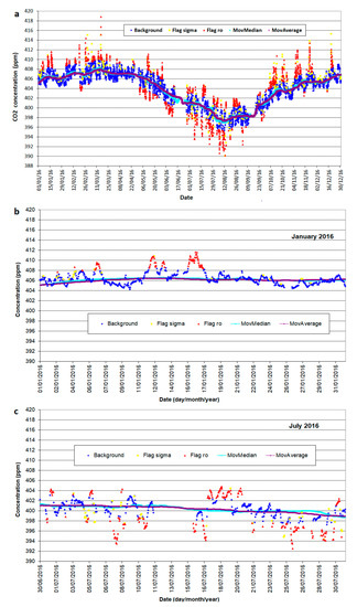
Figure 5.
The triangles represent all the raw hourly data measured in 2016 at PRS. The yellow triangles refer to the data that did not pass step 1 and the red ones to those that did not pass step 4. The blue triangles refer to the data that were considered background data. The curves in cyan and brown represent the moving median and moving average computed for 21 days of measurements, respectively, year 2016 (a), in January 2016 (b) and in July 2016 (c).
The choice of the σ, and parameters is based on experience gained over the years and represents a compromise so that only background measurements are retained and, at the same time, only a small number of hourly values are removed. Basically, the method tends to remove all the data that have excessively negative and positive peak values, compared to the trend curve (moving average).
One possible limitation of this procedure is represented by the number of acquired data. In other words, if there are long periods with missing data during the measurements, the method may not be effective in selecting the background data. For this reason, the curves related to the mobile median and moving average are calculated over a long period (21 days). However, other statistical methodologies also suffer from data deficiency problems.
The diurnal cycles were derived from the complete hourly dataset and from the selected background hourly data. A summer month (July) and a winter month (January), both related to the year 2016, are shown in Figure 6 as examples. The diurnal cycle does not appear in the January 2016 raw data (Figure 6a), while the effect of the BaDS filter is that of reducing the mean value by 0.42 ppm and the standard deviation by 0.52 ppm (Figure 6b). The daily cycle in the raw data shows a peak in the morning and a minimum in the afternoon in summer time (Figure 6c) and application of the BaDS filter reduces the daily cycle and the standard deviation by 0.90 ppm (Figure 6d). Similar results were also obtained for the other years.
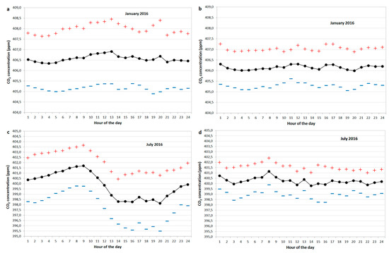
Figure 6.
Mean CO2 diurnal cycle recorded at PRS in January 2016 using non filtered data (black points), plus the standard deviation (red plus), minus the standard deviation (blue dashes) (a); and using filtered background data (b); as (a) but related to July 2016 (c); as (b) but related to July 2016 (d).
The PRS data does not seem to be influenced by the vegetation in winter (the diurnal cycle is absent), whereas it may be enriched by regional sources and sinks. The photosynthetic activity in summer is responsible for the diurnal cycle. The application of the BaDS filter reduces the effect of both photosynthetic activity and transport from regional sources and sinks. The absence of a diurnal cycle in the filtered data indicates that the application of the BaDS filter leads to the selection of data that are not affected by local sources and sinks.
In the Zhongshan station in the Antarctic, the monthly averaged deviations of the hourly mean CO2 mole fractions from the daily means are relatively low (about 1 ppm) throughout the entire year, thereby indicating that the observation point is not influenced by regional sources or sinks [50]. The monthly mean diurnal CO2 cycle at the Lampedusa station in the Mediterranean Sea (Italy) shows no cycle in winter and a very small diurnal cycle in summer, with mean hourly standard deviations of about 1.5 ppm in winter and 2.0 ppm in summer [41]. The monthly diurnal CO2 cycle at the Kasprowy Wierch mountain station (Poland) is only present in summer, with a peak-to-peak amplitude of about 5 ppm and a lower mean hourly standard deviation than 1 ppm in winter and of about 1 ppm in summer [54]. Thus, the comparison between the monthly diurnal CO2 cycle at PRS and the ones at other mountainous [54] or island [41] sites shows that the PRS observations are characterised by less variability, while the comparison with the Antarctic site shows the influence of the continental source and sink data on the PRS data.
The whole data set of the hourly averages, considered as background data, e.g., those resulting from the application of the BaDS filter, was then used to calculate the daily averages, and from these the monthly averages. As expected, the yearly cycle (year 2016 in Figure 7) shows a maximum at the beginning of spring (March) and a minimum in late summer (August).
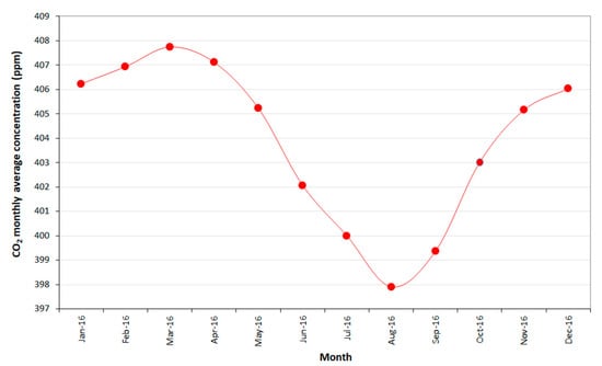
Figure 7.
Monthly average CO2 concentrations for the year 2016. The dots in red represent the background monthly averages.
5. The Time Series of the Monthly Averaged CO2 Background Concentrations
5.1. An Overview
The time series of the monthly data, from April 1989 to December 2018, is shown in Figure 8. The BaDS background data started in 1993, whereas flask analysis measurements were performed in the 1989–1997 years. During the overlapped period, that is, 1993–1997, the two independent measurements were comparable (the pink and red points in Figure 8).
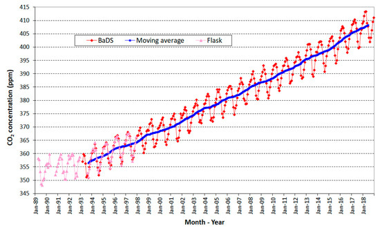
Figure 8.
Historical series of monthly averages of the CO2 background concentration gathered at Plateau Rosa by means of continuous measurements from March 1993 to December 2018 (red diamonds) and by means of weekly flask measurements from April 1989 to December 1997 (pink diamonds). The curve in the thick blue represents the centred moving average of an order of 12 of the background monthly values, applied only to continuous measurements.
The time series exhibits a combination of a long-term trend signal and a seasonal cycle with a maximum in March or April and a minimum in August each year, as pointed out in the previous section. The seasonal oscillations are due to terrestrial biospheric activities, and a mean peak-to-peak amplitude of about 10.4 ± 0.9 ppm may be observed. To estimate the growth rate, a linear fit of the background monthly data was performed. The growth rate is equal to 2.05 ± 0.03 ppm/year and is comparable with the global trend (1.9 to 2.1 ppm/year) computed for the 2002–2011 years by IPCC [1], and 2.24 ppm/year (for the last decade: 2008–2017) reported in the WMO Greenhouse Gas Bulletin (2018) [2]. The periodic annual signal was also filtered by computing a moving average with a step of 12 months (blue line in Figure 8). The linear fit of the moving average produced the same growth rate, that is, of 2.05 ppm/year.
5.2. Curve Fitting: The Long-Term Trend and The Seasonal Cycle
To extract more quantitative and analytical information on the cyclic behaviour and the growth rate of the CO2 concentration series, some periodic functions may be fitted to the monthly background mean values. Several authors (among them: [24,41,55,56,57]) fitted the background CO2 data with analytic curves that were the sum of linear, sinusoidal and eventually exponential terms representing the trend and the modulations of the CO2 concentrations.
The simplest equation that can be used has the following form:
where a, b and ci are numerical coefficients. Equation (1) is the sum of a linear term and sinusoidal terms, with , where is the period and the initial phase of each signal. The linear growth rate is evaluated by means of the coefficient b. The periods are usually estimated by means of spectral analysis [24].
If the growth rate is not constant, a function with an exponential term may be considered instead of the linear one [41]:
If the curve has an amplitude modulation, it is important to introduce an additional term: [55], with a fixed period of 12 months; this term represents the change rate of the annual cycle amplitude.
PRS CO2 Curve Fits
The PRS monthly background time series was analysed in order to identify the best curve to represent the data and its main features. The different fitting curves were compared by means of the RMSE (Root Mean Square Error) parameter between the data and the modelled curves.
The monthly CO2 concentration spectral power was computed to identify the Ti periods (Figure 9), and the presence of two main periodic signals was observed in the temporal series, with periods of 12 months and 6 months, respectively. The annual period corresponds to the natural vegetative cycle and the semi-annual one may be related to energy consumption [58].
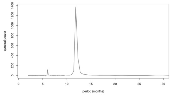
Figure 9.
Spectral analysis result of the mean background CO2 values.
Therefore, the fitting function (1) can be rewritten as:
where is the monthly CO2 concentration, t is the time in monthly units, and the coefficients , , and are constants. The and frequencies correspond to the annual and semi-annual periods (, ), and φ1 and φ2 are the initial annual and semi-annual phases. Table 1 contains the computed coefficients.

Table 1.
Values of the coefficients in Equation (2).
The corresponding growth rate deduced from the data (b coefficient, Table 2), expressed per year, becomes 2.06 ± 0.01 ppm/year, and is in agreement with the values computed using the linear fit of the monthly background data.
Table 2.
Values of significant coefficients in Equation (5).
The peak-to-peak amplitude of the first harmonic with the annual period was estimated with the c1 parameter and it is equal to 9.88 ± 0.18 ppm. This value is comparable with the seasonal amplitude (10.4 ± 0.9 ppm) computed at the beginning of this Section considering the mean peak-to-peak amplitude. The initial phase of the first harmonic identifies a maximum in March and a minimum in September.
The second harmonic, with a period of 6 months, has a lower peak-to-peak amplitude of 2.82 ± 0.18 ppm, maxima in May and November, and minima in August and February. The sum of these two harmonics has the effect of slightly increasing the curve amplitude and of correctly individuating three characteristics of the annual CO2 cycle: a maximum in April, a deep minimum in August and a “knee” (a decrease in the growth rate) that occurs in December.
The residuals range from −3 ppm to +3 ppm, with an RMSE value of 1.08 ppm.
At a global level, the amplitude of the seasonal cycle has increased since 1960, particularly north of 45° N, and it is mainly driven by positive trends in photosynthetic carbon uptake caused by the recent climate change and by the changing vegetation cover in the northern hemisphere [59].
A more complete fitting function was applied to explore a possible variation in the amplitude of the PRS time series with time:
The last term adds a linear increasing amplitude with annual periodicity. The same function was used by Sanchez et al. (2010) [41] to analyse CO2 data collected on an upper Spanish plateau at an altitude of 845 m a.s.l.
The introduction of the last additional term slightly improves the agreement between the measured data and the fitted curve, even though the variation in the residuals is almost negligible (RMSE = 1.07 ppm). Therefore, the vegetation cycle of CO2 at a high altitude seems to be characterised by a quasi-constant amplitude, at least for the analysed period.
As mentioned above, the growth behaviour may not be linear, and increasing values have been observed in the last few years. Artuso et al. (2009) [32] applied a fitting curve with an exponential term to analyse CO2 data collected at the Lampedusa station (Italy). According to this suggestion, an exponential term ( was used instead of a linear term (bt):
Figure 10a shows Equation (5) superimposed onto the monthly concentration values. The computed coefficients are written in Table 2.
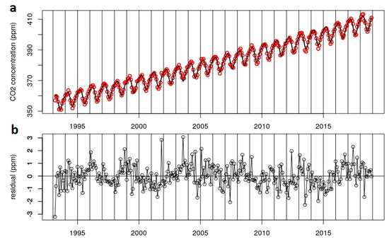
Figure 10.
Mean background monthly values at Plateau Rosa from 1993 to 2018 (red points), the exponential and periodic fitting functions (Equation (4)) (black line) (a), residuals between the data and fitted curve (b).
This curve with an exponential term is able to capture the spring maxima in the PRS CO2 data for the last few years that was instead underestimated with Equation (3) and Equation (4). The c1 and c2 parameters have comparable values with the corresponding ones in Equation (3) and in Table 1. The amplitude of the last term () grows in time, but it is still relatively small (about 0.78 ppm) for 2018, as a consequence of the slight variation in amplitude of the PRS CO2 data.
The RMSE value of the residuals (shown in Figure 10b) is 0.86 ppm, which is lower than the one obtained using Equation (2); therefore, the exponential term improves the agreement between the model and the data.
As many authors have used 4 harmonics for their fitting curve [24,60], two sinusoidal terms, with periods of 4 and 3 months, were added to Equation (5). In this test, the residual values were between −3 and 3 ppm and the RMSE parameter results were unchanged (0.86 ppm).
Another test was applied to the monthly CO2 means from 1989 to 2018, considering the background monthly data from 1993 to 2018 obtained using the BaDS procedure together with the monthly averages computed from flask observation without using a filtering selection (pink and red diamonds in Figure 8). An exponential fit with 4 harmonics, as in the previous test, was applied (Figure 11), and a good agreement was obtained for the whole period and also for the 1989–1993 years. In this case, the RMSE value was 1.03 ppm, as a consequence of the enhanced variability in the first years, due to more uncertainty in the data.
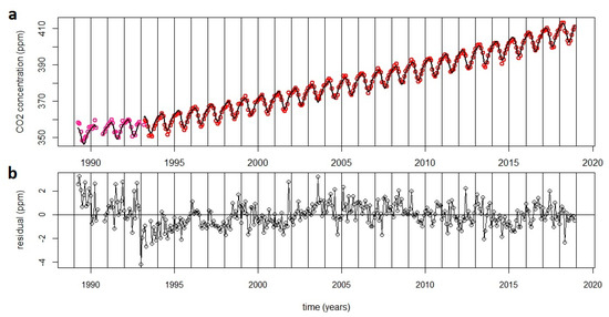
Figure 11.
Monthly means at Plateau Rosa from 1989 to 1993 (pink points) and from 1993 to 2018 (red points), the exponential and periodic fitting functions (4 harmonics) (black line) (a), residual between the data and fitted curve (b).
6. Correlation between the Growth Rate and the Natural Indexes
Natural climatic variability may be observed in the CO2 background concentration, as reported in many studies, from the pioneering work of Bacastow (1976) [61]. The correlation between the annual and monthly variability of the growth rate and the ENSO (El Niño Southern Oscillation) is investigated in this section. The El Niño Southern Oscillation is the most important coupled ocean-atmosphere phenomenon responsible for global climate variability at inter-annual time scales. As already mentioned by many authors (among others: [1,14,62]), a positive phase of ENSO is generally associated with an enhanced land CO2 source, while a negative phase (La Niña) is associated with an enhanced land CO2 sink. In fact, the reduction in the sea-to-air CO2 flux during an ENSO period may be responsible for an increase in the atmospheric CO2 content in the same period.
In the 1993–2018 period, very important ENSO events occurred in 1997–1998 and in 2015–2016, and other episodes, characterised by moderate intensities, took place in 1994–1995, 2002–2003 and in 2009–2010.
6.1. Annual Mean Growth Rate
The annual growth rate was computed with the algorithm used by NOAA (National Oceanic and Atmospheric Administration) for the data collected at the Mauna Loa station [24]. The method uses the monthly means, corrected for the averaged seasonal cycle, computes the averages of the four November, December, January and February months every year and associates this value to 1 January. The estimate for the annual mean growth rate is then obtained by evaluating the differences between the averages.
The twelve-month centred moving mean value was considered for the PRS data, and the same method was applied. The annual mean growth rates are shown in Figure 11. The mean growth rate is equal to 2.1 ± 0.6 ppm/year. A comparison with the Mauna Loa monthly growth rates [63] for the same years shows a good agreement, with comparable maximum and minimum values for the same years (Figure 12).
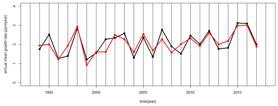
Figure 12.
CO2 annual growth rate at the Plateau Rosa station (black line and points) and at the Mauna Loa station (red line and points) [63].
High values of the annual growth rate identify ENSO events. An inspection of Figure 12 shows that the three highest annual growth rates in the PRS data, with higher values than 2.8 ppm/year, were recorded in 1998, 2015 and 2016, when the two most intense ENSO periods occurred.
Moreover, Betts et al. (2016) [64] predicted that, as a consequence of the 2015–2016 ENSO event, the CO2 concentration at the Mauna Loa station would remain above 400 ppm all year round, and that the annual mean CO2 growth rate would be exceptional, that is, 3.15 ± 0.53 ppm yr−1 between 2015 and 2016. In the same period, the annual PRS growth rates were the highest of the series (3.12 ppm/year and 3.10 ppm/year, respectively—Figure 12), thus showing that the PRS data were also influenced by the El Niño event.
6.2. Monthly Mean Growth Rate
ENSO events may also be individuated from the monthly mean growth rate series by means of a correlation with the Southern Oscillation Index (SOI). This index is a measure of the large-scale fluctuations in air pressure that occur between the western and eastern tropical Pacific Ocean during El Niño episodes. This index is traditionally calculated on the basis of the differences in air pressure between Tahiti and Darwin, Australia. SOI index values are negative during El Niño events. The SOI index is available in [65].
The PRS monthly mean growth rates (Figure 13) were calculated from the differences between the same months from adjacent years, and the result were attributed to the central year: for example, the grow rate for September 1993 is the difference between the concentrations in March 1993 and March 1994 [66].
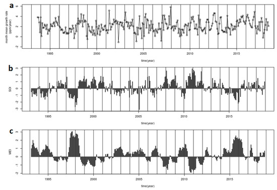
Figure 13.
Monthly mean growth rate of the monthly CO2 background PRS series (a), SOI (b), MEI (c).
As expected, the carbon dioxide growth rate at the PRS station and the SOI index (Figure 13) are negatively correlated. The maximum anti-correlation occurs between the monthly grow rate and the SOI, with a delay of 4 months (cross-correlation coefficient equal to 0.31, confidence correlation of 95% equal to 0.11). Similar analyses conducted with data collected at the Monte Cimone and Lampedusa stations, in the 1979–1991 and 1997–2000 periods, produced delays of 7 and 9 months [20,67], respectively.
The Multivariate ENSO Index (MEI) is computed using six observed variables over the tropical Pacific [68]: the sea-level pressure, the zonal and meridional components of the surface wind, the sea surface temperature, the surface air temperature and the total cloudiness fraction of the sky. If more variables were integrated, the MEI index would be less vulnerable to occasional data errors. ENSO events occur during positive phases of the MEI index, and the inter-annual sea-air CO2 flux variability is significantly anti-correlated with the MEI index at almost all longitudes [69]. Therefore, increased CO2 growth rate values may be expected during positive MEI phases.
In the 1993–2016 period, the two important ENSO events of 1997–1998 and 2015–2016 correspond to higher MEI index values than 2. The other events (1994–1995, 2002–2003, 2009–2010) are also identifiable in the MEI index (Figure 13).
The PRS growth rate and the MEI index may be seen to be correlated and the maximum agreement occurs for a lag of 4 months (cross-correlation coefficient equal to 0.31, confidence correlation of 95% equal to 0.11).
7. Conclusions
The atmospheric CO2 concentration has been measured at the Plateau Rosa site in the north-western Alps since 1989, and in a continuous mode since 1993. The complete series now covers 30 years, and it is thus suitable for climatological studies.
The measurements have been performed using the most up-to-date time measurement techniques and the data have been compared since the instrumentation was changed. The data have been analysed using a filtering technique, called BaDS, to select background data and to build the monthly PRS background data series.
The main characteristics of the monthly PRS background series are: trend (2.05 ± 0.03 ppm/year), peak-to-peak amplitude of the seasonal oscillation (10.4 ± 0.9 ppm), maximum and minimum times (March-April and August, respectively). The series shows a linear (or exponential) growth rate as a result of anthropogenic emissions, a first harmonic with a period of one year, due to seasonal oscillations, a second harmonic with a 6-month period, and a small variation in amplitude (0.78 ppm in 25 years). The addition of two more harmonics (periods of 4 and 3 months) has not significantly improved the agreement between the modelled and observed values. Furthermore, the complete series of monthly data (1989–2018), including the observations performed with flasks in 1989–1993, is well represented by the curve composed of an exponential term, 4 sinusoidal harmonics and a modulation amplitude term.
Moreover, the historical series also contains traces of climatic variability at a planetary scale: in fact, the annual growth rates of the PRS series are in agreement with those observed at the Mauna Loa station, and are able to identify the ENSO years. The monthly growth rates appear to be correlated with some climatic indexes (SOI and MEI), with a lag of 4 months.
The position of the station, that is, in a mountain environment and at very high altitude, the constancy of the continuous measurements, the appropriate instrumentation, which collects reliable values, and good-practice measurement rules have permitted an important long-term series of background atmospheric CO2 concentrations to be obtained.
The Plateau Rosa measurement station, as well as other measurement stations in international monitoring networks, provides fundamental data that may be used to evaluate how the commitment to containing CO2 emissions, which has been undertaken by policymakers throughout the world, will be effective in containing global warming. At the same time, it provides data of particular importance for the modelling of carbon cycles and for the evaluation of CO2 sources and sinks by means of inverse modelling.
Author Contributions
Conceptualisation, F.A. and S.F.; methodology, F.A. and S.F.; software, F.A., S.F. and A.L.; validation, F.A. and A.L.; formal analysis, F.A., C.C. and S.F.; investigation, F.A. and S.F.; data curation, F.A., Daniela Heltai and A.L.; writing—original draft preparation, F.A. and S.F.; writing—review and editing, F.A., C.C. and S.F.; supervision, F.A.; project administration, F.A.; funding acquisition, F.A.
Funding
The experimental activities on going to Plateau Rosa monitoring station has been financed by the Research Fund for the Italian Electrical System under the Contract Agreement between RSE S.p.A. and the Ministry of Economic Development—General Directorate for the Electricity Market, Renewable Energy and Energy Efficiency, Nuclear Energy in compliance with the Decree of 8 March 2006. Partial financing has also been obtained from NextDATA (MIUR), through a contribution of the CNR-ISAC, for the measurements carried out during the year 2014 and from 2017 to 2018.
Acknowledgments
We would like to thank the CNR (National Research Council) for allowing the use of the Testa Grigia Laboratory, where the Plateau Rosa monitoring station measurement equipment is operational. The authors would also like to thank the anonymous reviewers for their important suggestions that have helped them reach the final version of this article.
Conflicts of Interest
The authors declare no conflict of interest. The funders played no role in the design of the study; in the collection, analyses or in the interpretation of the data; in the writing of the manuscript, or in the decision to publish the results.
References
- IPCC. Climate Change 2013: The Physical Science Basis. In Contribution of Working Group I to the Fifth Assessment Report of the Intergovernmental Panel on Climate Change; Cambridge University Press: Cambridge, UK; New York, NY, USA, 2013; p. 1535. [Google Scholar]
- WMO Greenhouse Gas Bulletin. The State of Greenhouse Gases in the Atmosphere Based on Global Observations through 2017. WMO No. 14. 22 November 2018. Available online: https://library.wmo.int/doc_num.php?explnum_id=5455 (accessed on 18 June 2019).
- Advanced Global Atmospheric Experiment. Available online: https://agage.mit.edu (accessed on 18 June 2019).
- Global Greenhouse Gas Reference Network. Available online: https://www.esrl.noaa.gov/gmd/ccgg (accessed on 18 June 2019).
- Word Data Centre for Greenhouse Gases. Available online: https://gaw.kishou.go.jp (accessed on 18 June 2019).
- Integrated Carbon Observation System. Available online: https://www.icos-ri.eu/icos-national-networks (accessed on 18 June 2019).
- WMO Greenhouse Gas Bulletin. The State of Greenhouse Gases in the Atmosphere Based on Global Observations through 2012. WMO No. 9. 6 November 2013. Available online: https://library.wmo.int/doc_num.php?explnum_id=7288 (accessed on 18 June 2019).
- Longhetto, A.; Apadula, F.; Bacci, P.; Bonelli, P.; Cassardo, C.; Ferrarese, S.; Giraud, C.; Vannini, C. A study of greenhouse gases and air trajectories at Plateau Rosa. Il Nuovo Cim. C 1995, 18, 583–601. [Google Scholar] [CrossRef]
- Longhetto, A.; Ferrarese, S.; Cassardo, C.; Giraud, C.; Apadula, F.; Bacci, P.; Bonelli, P.; Marzorati, A. Relationships between atmospheric circulation patterns and CO2 greenhouse–gas concentration levels in the Alpine troposphere. Adv. Atmos. Sci. 1997, 14, 309–322. [Google Scholar] [CrossRef]
- Ferrarese, S.; Longhetto, A.; Cassardo, C.; Apadula, F.; Bertoni, D.; Giraud, C.; Gotti, A. A study of seasonal and yearly modulation of carbon dioxide sources and sinks, with a particular attention to the Boreal Atlantic Ocean. Atmos. Environ. 2002, 36, 5517–5526. [Google Scholar] [CrossRef]
- Ferrarese, S. Sensitivity test of a source-receptor model. Il Nuovo Cim. 2002, 25, 501–511. [Google Scholar]
- Apadula, F.; Gotti, A.; Pigini, A.; Longhetto, A.; Rocchetti, F.; Cassardo, C.; Ferrarese, S.; Forza, R. Localization of source and sink regions of carbon dioxide through the method of the synoptic air trajectory statistics. Atmos. Environ. 2003, 37, 3757–3770. [Google Scholar] [CrossRef]
- Ferrarese, S.; Apadula, F.; Bertiglia, F.; Cassardo, C.; Ferrero, A.; Fialdini, L.; Francone, C.; Heltai, D.; Lanza, A.; Longhetto, A.; et al. Inspection of high–concentration CO2 events at the Plateau Rosa Alpine station. Atmos. Pollut. Res. 2015, 6, 415–427. [Google Scholar] [CrossRef]
- Peylin, P.; Rayner, P.J.; Bousquet, P.; Carouge, C.; Hourdin, F.; Heinrich, P.; Ciais, P. AEROCARB contributors: Daily CO2 flux estimates over Europe from continuous atmospheric measurements: 1, inverse methodology. Atmos. Chem. Phys. 2005, 5, 3173–3186. [Google Scholar] [CrossRef]
- Peters, W.; Krol, M.C.; van Der Werf, G.R.; Houweling, S.; Jones, C.D.; Hughes, J.; Schaefer, K.; Masarie, K.A.; Jacobson, A.R.; Miller, J.B.; et al. Seven years of recent European net terrestrial carbon dioxide exchange constrained by atmospheric observations. Glob. Chang. Biol. 2010, 16, 1317–1337. [Google Scholar] [CrossRef]
- Broquet, G.; Chevallier, F.; Bréon, F.-M.; Kadygrov, N.; Alemanno, M.; Apadula, F.; Hammer, S.; Haszpra, L.; Meinhardt, F.; Morguí, J.A.; et al. Regional inversion of CO2 ecosystem fluxes from atmospheric measurements: Reliability of the uncertainty estimates. Atmos. Chem. Phys. 2103, 13, 9039–9056. [Google Scholar] [CrossRef]
- Climatological Temperature at PRS. Available online: http://clima.meteoam.it/web_clima_sysman/Clino6190/CLINO052.txt (accessed on 18 June 2019).
- WMO X2007 Reference Scale. Available online: http://www.esrl.noaa.gov/gmd/ccl/co2_scale.html (accessed on 19 July 2019).
- Komhyr, W.D.; Harris, T.B.; Waterman, L.S.; Chin, J.F.S.; Thoning, K.W. Atmospheric carbon dioxide at Mauna Loa Observatory, 1, NOAA Global Climatic Measurement with a Nondispersive Infrared Analyser, 1974–1985. J. Geophys. Res. 1989, 94, 8533–8547. [Google Scholar] [CrossRef]
- Cundari, V.; Colombo, T.; Ciattaglia, L. Thirteen years of atmospheric carbon dioxide measurements at Mt. Cimone station, Italy. Il Nuovo Cim. C 1995, 18, 33–47. [Google Scholar] [CrossRef]
- Laurent, O. ICOS Atmospheric Station Specifications, Version 1.2; August 2016. Available online: https://icos-atc.lsce.ipsl.fr/filebrowser/download/27251 (accessed on 20 May 2019).
- Observation Package. Available online: https://www.esrl.noaa.gov/gmd/ccgg/obspack/labinfo.html (accessed on 18 June 2019).
- Ruckstuhl, A.F.; Henne, S.; Reimann, S.; Steinbacher, M.; Vollmer, M.K.; O’Doherty, S.; Buchmann, B.; Hueglin, C. Robust extraction of baseline signal of atmospheric trace species using local regression. Atmos. Meas. Technol. 2012, 5, 2613–2624. [Google Scholar] [CrossRef]
- Thoning, K.; Tans, P.; Komhyr, W. Atmospheric Carbon Dioxide at Mauna Loa Observatory. 2. Analysis of the NOAA GMCC Data, 1974–1985. J. Geophys. Res. 1989, 94, 8549–8565. [Google Scholar] [CrossRef]
- Novelli, P.; Masarie, K.; Lang, P. Distributions and recent changes of carbon monoxide in the lower troposphere. J. Geophys. Res. 1998, 103, 19015–19033. [Google Scholar] [CrossRef]
- Schuepbach, E.; Friedli, T.; Zanis, P.; Monks, P.; Penkett, S. State space analysis of changing seasonal ozone cycles (1988–1997) at Jungfraujoch (3580 m above sea level) in Switzerland. J. Geophys. Res. 2001, 106, 20413–20427. [Google Scholar] [CrossRef]
- Novelli, P.; Masarie, K.; Lang, P.; Hall, B.; Myers, R.; Elkins, J. Reanalysis of tropospheric CO trends: Effect of the 1997–1998 wildfires. J. Geophys. Res. 2003, 108, 4464. [Google Scholar] [CrossRef]
- Zellweger, C.; Hüglin, C.; Klausen, J.; Steinbacher, M.; Vollmer, M.; Buchmann, B. Inter-comparison of four different carbon monoxide measurement techniques and evaluation of the long-term carbon monoxide time series of Jungfraujoch. Atmos. Chem. Phys. 2009, 9, 3491–3503. [Google Scholar] [CrossRef]
- Moody, J.L.; Samson, P.J. The influence of atmospheric transport on precipitation chemistry at two sites in the midwestern United States. Atmos. Environ. 1989, 23, 2117–2132. [Google Scholar] [CrossRef]
- Harris, J.M.; Kahl, J.D. A descriptive atmospheric transport climatology for the Mauna Loa Observatory, using clustered trajectories. J. Geophys. Res. 1990, 95, 13651–13667. [Google Scholar] [CrossRef]
- Prinn, R.G.; Huang, J.; Weiss, R.F.; Cunnold, D.M.; Fraser, P.J.; Simmonds, P.G.; McCulloch, A.; Harth, C.; Salameh, P.; O’Doherty, S.; et al. Evidence for substantial variations of atmospheric hydroxyl radicals in the past two decades. Science 2001, 292, 1882–1888. [Google Scholar] [CrossRef]
- Cox, M.L.; Sturrock, G.A.; Fraser, P.J.; Siems, S.T.; Krummel, P.B. Identification of Regional Sources of Methyl Iodide from AGAGE Observations at Cape Grim, Tasmania. J. Atmos. Chem. 2005, 50, 59–77. [Google Scholar] [CrossRef]
- Reimann, S.; Manning, A.J.; Simmonds, P.G.; Cunnold, D.M.; Wang, R.H.J.; Li, J.; McCulloch, A.; Prinn, R.G.; Huang, J.; Weiss, R.F.; et al. Low European methyl chloroform emissions inferred from long-term atmospheric measurements. Nature 2005, 433, 506–508. [Google Scholar] [CrossRef] [PubMed]
- Greally, B.R.; Manning, A.J.; Reimann, S.; McCulloch, A.; Huang, J.; Dunse, B.L.; Simmonds, P.G.; Prinn, R.G.; Fraser, P.J.; Cunnold, D.M.; et al. Observations of 1,1-difluoroethane (HFC-152a) at AGAGE and SOGE monitoring stations in 1994–2004 and derived global and regional emission estimates. J. Geophys. Res. 2007, 112. [Google Scholar] [CrossRef]
- Graziosi, F.; Arduini, J.; Furlani, F.; Giostra, U.; Cristofanelli, P.; Fang, X.; Hermanssene, O.; Lunder, C.; Maenhout, G.; O’Doherty, S.; et al. European emissions of the powerful greenhouse gases hydrofluorocarbons inferred from atmospheric measurements and their comparison with annual national reports to UNFCCC. Atmos. Environ. 2017, 158, 85–97. [Google Scholar] [CrossRef]
- Ryall, D.B.; Maryon, R.H.; Derwent, R.G.; Simmonds, P.G. Modelling long-range transport of CFCs to Hace Head, Ireland. Q. J. Roy Meteorol. Soc. 1998, 124, 417–446. [Google Scholar] [CrossRef]
- Balzani Lööv, J.M.; Henne, S.; Legreid, G.; Staehelin, J.; Reimann, S.; Prevot, A.S.H.; Steinbacher, M.; Vollmer, M.K. Estimation of background concentrations of trace gases at the Swiss Alpine site Jungfraujoch (3580 m asl). J. Geophys. Res. 2008, 113. [Google Scholar] [CrossRef]
- Carpenter, L.; Green, T.; Mills, G.; Bauguitte, S.; Penkett, S.; Zanis, P.; Schuepbach, E.; Schmidbauer, N.; Monks, P.; Zellweger, C. Oxidized nitrogen and ozone production efficiencies in the springtime free troposphere over the Alps. J. Geophys. Res. 2000, 105, 14547–14559. [Google Scholar] [CrossRef]
- Zanis, P.; Ganser, A.; Zellweger, C.; Henne, S.; Steinbacher, M.; Staehelin, J. Seasonal variability of measured ozone production efficiencies in the lower free troposphere of Central Europe. Atmos. Chem. Phys. 2007, 7, 223–236. [Google Scholar] [CrossRef]
- Zhang, F.; Zhou, L.; Conway, T.J.; Tans, P.P.; Wang, Y. Short-term variations of atmospheric CO2 and dominant causes in summer and winter: Analysis of 14-year continuous observational data at Waliguan, China. Atmos. Environ. 2013, 77, 140–148. [Google Scholar] [CrossRef]
- Artuso, F.; Chamard, P.; Piacentino, S.; Sferlazzo, D.M.; De Silvestri, L.; di Sarra, A.; Meloni, D.; Monteleone, F. Influence of transport and trends in atmospheric CO2 at Lampedusa. Atmos. Environ. 2009, 43, 3044–3051. [Google Scholar] [CrossRef]
- Derwent, R.; Simmonds, P.; O’Doherty, S.; Ciais, P.; Ryall, D. European source strengths and northern hemisphere baseline concentrations of radiatively active trace gases at Mace Head, Ireland. Atmos. Environ. 1998, 32, 3703–3715. [Google Scholar] [CrossRef]
- Forrer, J.; Rüttimann, R.; Schneiter, D.; Fischer, A.; Buchmann, B.; Hofer, P. Variability of trace gases at the high-Alpine site Jungfraujoch caused by meteorological transport processes. J. Geophys. Res. 2000, 105, 12241–12251. [Google Scholar] [CrossRef]
- Zellweger, C.; Forrer, J.; Hofer, P.; Nyeki, S.; Schwarzenbach, B.; Weingartner, E.; Ammann, M.; Baltensperger, U. Partitioning of reactive nitrogen (NOy) and dependence on meteorological conditions in the lower free troposphere. Atmos. Chem. Phys. 2003, 3, 779–796. [Google Scholar] [CrossRef]
- Henne, S.; Furger, M.; Prevot, A. Climatology of mountain venting-induced elevated moisture layers in the lee of the Alps. J. Appl. Meteorol. 2005, 44, 620–633. [Google Scholar] [CrossRef]
- Ryall, D.B.; Derwent, R.; Manning, A.; Simmonds, P.; O’Doherty, S. Estimating source regions of European emissions of trace gases from observations at Mace Head. Atmos. Environ. 2001, 35, 2507–2523. [Google Scholar] [CrossRef]
- Hirdman, D.; Sodemann, H.; Eckhardt, S.; Burkhart, J.F.; Jefferson, A.; Mefford, T.; Quinn, P.K.; Sharma, S.; Ström, J.; Stohl, A. Source identification of short-lived air pollutants in the Arctic using statistical analysis of measurement data and particle dispersion model output. Atmos. Chem. Phys. 2010, 10, 669–693. [Google Scholar] [CrossRef]
- Yuan, Y.; Ries, L.; Petermeier, H.; Steinbacher, M.; Gómez-Peláez, A.J.; Leuenberger, M.C.; Schumacher, M.; Trickl, T.; Couret, C.; Meinhardt, F.; Menzel, A. Adaptive selection of diurnal minimum variation: A statistical strategy to obtain representative atmospheric CO2 data and its application to European elevated mountain stations. Atmos. Meas. Technol. 2018, 11, 1501–1514. [Google Scholar] [CrossRef]
- Uglietti, C.; Leuenberger, M.; Brunner, D. European source and sink areas of CO2 retrieved from Lagrangian transport model interpretation of combined O2 and CO2 measurements at the high alpine research station Jungfraujoch. Atmos. Chem. Phys. 2011, 11, 8017–8036. [Google Scholar] [CrossRef]
- Sun, Y.; Bian, L.; Tang, J.; Gao, Z.; Lu, C.; Schnell, R.C. CO2 monitoring and background mole fraction at Zhongshan station, Antarctica. Atmosphere 2014, 5, 686–698. [Google Scholar] [CrossRef]
- Schmidt, M.; Graul, R.; Sartorius, H.; Levin, I. The Schauinsland CO2 record: 30 years of continental observations and their implications for the variability of the European CO2 budget. J. Geophys. Res. 2003, 108. [Google Scholar] [CrossRef]
- Valentino, F.L.; Leuenberger, M.; Uglietti, C.; Sturm, P. Measurements and trend analysis of O2, CO2 and δ13C of CO2 from high altitude research station Junfgraujoch, Switzerland—A comparison with the observations from the remote site Puy de Dome, France. Sci. Total Environ. 2008, 391, 203–210. [Google Scholar] [CrossRef] [PubMed]
- Fang, X.S.; Zhou, L.X.; Tans, P.P.; Cias, P.; Steinbacher, M.; Xu, L.; Luan, T. In situ measurements of atmospheric CO2 at the four WMO/GAW stations in China. Atmos. Chem. Phys. 2014, 14, 2541–2554. [Google Scholar] [CrossRef]
- Necki, J.; Schmidt, M.; Rozanski, K.; Zimnoch, M.; Korus, A.; Lasa, J.; Graul, R.; Levin, I. Six-years record of atmospheric carbon dioxide and methane at a high-altitude mountain site in Poland. Tellus B 2003, 55, 94–104. [Google Scholar] [CrossRef]
- Sanchez, M.L.; Perez, I.A.; Garcia, M.A. Study of CO2 variability at different temporal scales recorded in a rural Spanish site. Agric. For. Meteorol. 2010, 150, 1168–1173. [Google Scholar] [CrossRef]
- Wu, J.; Guan, D.; Yuan, F.; Yang, H.; Wang, A.; Jin, C. Evolution of atmoaspheric carbon dioxide concentration at different temporal scales recorded in a tall forest. Atmos. Environ. 2012, 61, 9–14. [Google Scholar] [CrossRef]
- Timokhina, A.V.; Prokushkin, A.S.; Onuchin, A.A.; Panov, A.V.; Kofman, G.B.; Heimann, M. Variability of ground CO2 concentration in the middle taiga subzone of the Yenisei region of Siberia. Russ. J. Ecol. 2015, 46, 143–151. [Google Scholar] [CrossRef]
- Erickson, D.J., III; Mills, R.T.; Gregg, J.; Blasing, T.J.; Hoffman, F.M.; Andres, R.H.; Devries, M.; Zhu, Z.; Kawa, S.R. An estimate of monthly global emissions of anthropogenic CO2: Impact on the seasonal cycle of atmospheric CO2. J. Geophys. Res. 2008, 113, G01023. [Google Scholar] [CrossRef]
- Forkel, M.; Carvalhais, N.; Rödenbeck, C.; Keeling, R.; Heimann, M.; Thonicke, K.; Zaehle, S.; Reichstein, M. Enhanced Seasonal CO2 Exchange Caused by Amplified Plant Productivity in Northern Ecosystems. Science 2016, 351, 696–699. [Google Scholar] [CrossRef]
- Curve Fitting. Available online: https://www.esrl.noaa.gov/gmd/ccgg/mbl/crvfit/crvfit.html (accessed on 18 June 2019).
- Bacastow, R.B. Modulation of atmospheric carbon dioxide by the Southern Oscillation. Nature 1976, 261, 116–118. [Google Scholar] [CrossRef]
- Jones, C.D.; Cox, P.M. Modeling the volcanic signal in the atmospheric CO2 record. Glob. Biogeochem. Cycles 2001, 15, 453–465. [Google Scholar] [CrossRef]
- Annual Growths Rate at Mauna Loa Station. Available online: www.esrl.noaa.gov/gmd/ccgg/trends/gr.html (accessed on 27 May 2019).
- Betts, R.A.; Jones, C.D.; Knight, J.R.; Keeling, R.F.; Kennedy, J.J. El Niño and a record CO2 rise. Nat. Clim. Chang. 2016, 6, 806–810. [Google Scholar] [CrossRef]
- SOI Index. Available online: www.cpc.ncep.noaa.gov/data/indices/soi (accessed on 27 May 2019).
- Patra, P.K.; Maksyutov, S.; Nakazawa, T. Analysis of atmospheric CO2 growth rates at Mauna Loa using CO2 fluxes derived from an inverse model. Tellus B 2005, 57, 357–365. [Google Scholar] [CrossRef]
- Chamard, P.; Thiery, F.; Di Sarra, A.; Ciattaglia, L.; De Silvestri, L.; Grigioni, F.; Monteleone, F.; Piacentino, S. Interannual variability of atmospheric CO2 in the Mediterranean: Measurements at the island of Lampedusa. Tellus B 2003, 55, 83–93. [Google Scholar] [CrossRef]
- MEI Index. Available online: https://www.esrl.noaa.gov/psd/enso/mei.old/table.html (accessed on 27 May 2019).
- Rödenbeck, C.; Bakker, D.C.E.; Metzl, N.; Olsen, A.; Sabine, C.; Cassar, N.; Reum, F.; Keeling, R.F.; Heimann, M. Interannual sea–air CO2 flux variability from an observation-driven ocean mixed-layer scheme. Biogeosciences 2014, 11, 4599–4613. [Google Scholar] [CrossRef]
© 2019 by the authors. Licensee MDPI, Basel, Switzerland. This article is an open access article distributed under the terms and conditions of the Creative Commons Attribution (CC BY) license (http://creativecommons.org/licenses/by/4.0/).