Application of GCM Bias Correction to RCM Simulations of East Asian Winter Climate


APEC Climate Center (APCC), Busan 48058, Korea
*
Author to whom correspondence should be addressed.
Atmosphere 2019, 10(7), 382; https://doi.org/10.3390/atmos10070382
Submission received: 28 May 2019
/
Revised: 20 June 2019
/
Accepted: 4 July 2019
/
Published: 9 July 2019
(This article belongs to the Section Meteorology)
Abstract
:Both the global circulation model (GCM) and regional climate model (RCM) simulations suffer from model biases that eventually result in significant errors in regional forecasts. This model bias issue is addressed using the bias correction approach. This study examines the influence of bias correction on the performance of downscaling simulations of the East Asian winter climate using the Global/Regional Integrated Model system (GRIMs). To assess the bias correction approach, we conducted three sets of simulations for 25 winters (December to February) from 1982 to 2006 over East Asia. The GRIMs were forced by the (1) National Centers for Environmental Prediction (NCEP) Department of Energy (DOE) reanalysis data, (2) original NCEP Climate Forecast System (CFS) data, and (3) bias-corrected CFS data. The GCM climatological means were adjusted based on the NCEP–DOE reanalysis data. The bias correction method was applied to zonal and meridional wind, temperature, geopotential height, specific humidity, and sea surface temperature of the CFS data. The GCM-driven experiments with/without bias correction were compared with the reanalysis-driven simulation. The results of this comparison suggest that the application of bias correction improves the downscaled climate in terms of the climatological mean, inter-annual variability, and extreme events owing to the elimination of errors in large-scale circulations. The effect of bias correction on the simulated extreme event is not as significant as those on the climatological mean and inter-annual variability, but the increased skill appears to be a clue for potential use for predicting extreme events.
1. Introduction
The fully coupled general circulation model (GCM) is an ultimate tool for seasonal climate prediction. The dynamical prediction system has been generally used for operational medium-range weather and seasonal prediction [1,2,3]. These dynamical prediction models are fully coupled climate system models that include the dynamics and physics for atmosphere, land, ocean, and sea–ice interactions. However, the resolution of GCMs is generally too coarse (approximately 1° for the atmosphere) to directly represent high-impact weather at local scales, although they can resolve synoptic-scale disturbance. The dynamical downscaling pioneered by Giorgi and Bates [4] is believed to produce more generally applicable, physically-based results. This downscaling approach is used to obtain the geographical distribution and time evolution of small-scale features, given large-scale coarse-resolution analyses, forecasts, or simulations as added values [5,6,7,8,9].
Many studies have presented seasonal climate simulations for specific regions using regional climate models (RCMs) forced by GCM simulations, which contain higher spatial resolutions and various physical parameterizations [7,8,10,11]. For example, Yoon et al. [7] conducted dynamical downscaling with GCM seasonal prediction using seven regional climate models for the conterminous U.S. region. They suggested that the RCMs show added value in seasonal prediction application although its improvement depends on the region, variable, and forecast lead time. Xue et al. [11] have reviewed studies related to the regional dynamical downscaling in seasonal prediction. They mentioned that dynamic downscaling using RCM can add value on intra-seasonal and seasonal prediction and future projection as compared to the GCM or reanalysis [12,13,14].
Various GCM bias correction methods using a mean bias correction have been developed over the past decade [15,16,17,18] and have been proven to improve performance and reduce uncertainties in RCMs [19,20,21]. The GCM bias correction methods are applied to a regional prediction or future projection because the GCMs are well-known for having large systematic sea surface temperature (SST) biases and atmospheric circulation biases. For example, Xu and Yang [19] showed that a dynamical downscaling with GCM bias corrections results in significant improvements in both the mean climate and climate variability. Mayer and Jin [20] mentioned that dynamical downscaling with bias correction for temperature results in the elimination of long-term biases and improvement of the seasonal climate characteristics. Their studies show that bias correction plays a role in reproducing more realistic climate simulations owing to the reduction of dynamical imbalances within the lateral boundary condition.
Meanwhile, the East Asian winter monsoon (EAWM) is well-known as a significant climate feature over East Asia during boreal winter. General characteristics of the winter monsoon and cold surges have been examined in many studies [22,23]. However, little attention has been given to skill in predicting the EAWM owing to a wide range of skills in predicting the EAWM of seasonal forecast models [24,25,26,27,28]. In some studies, efforts were made to improve the seasonal prediction skill via an ocean–atmosphere coupling process of the dynamical forecasting system [26] and the post-processing of forecast outputs using multi-model ensembles [25]. However, a few studies have been focused on the effect of dynamical downscaling with GCM bias correction on dynamically-downscaled RCM simulations of the EAWM.
Many evaluation works have been based on reanalysis-driven RCM simulations [29,30,31,32,33]. The differences between the simulations with reanalysis boundary conditions and observations can be regarded as RCM errors if we take the reanalysis data as the “perfect” boundary condition. The experiments forced by the GCM boundary conditions usually result in larger biases due to the GCM biases, which is an additional source of error in RCM simulations. Therefore, differences between the GCM-driven simulations and observations result from both the GCM and RCM biases. These biases could have the same or opposite sign. The biases with the opposite sign would offset each other. In this case, the simulation with the GCM boundary data may be closer to observation than the simulation with the reanalysis boundary, which does not mean that the GCM-driven simulation is actually better than the reanalysis-driven simulation.
The objective of this study is to assess the effect of GCM bias correction in dynamical downscaling using RCM on East Asian winter climate prediction. For this purpose, the GCM-driven simulations will be compared with reanalysis-driven simulations rather than with observations. The results are investigated based on a climatological seasonal state, an inter-annual variation, and extreme events. In the following sections, the bias correction method, the model used, and the simulations conducted in our study are described. The obtained results are presented in Section 3. Finally, the summary and conclusion of this study are presented in Section 4.
2. Method and Experimental Design
2.1. General Circulation Model (GCM) Bias Correction Method
In previous studies [16,34,35], two bias correction methods, ensemble average (Equation (1)) and anomaly nesting (Equation (2)), have been extensively used:
where, N is the number of ensemble members, i denotes each member, and the subscripts E and A represent the ensemble average and anomaly nesting, respectively. Furthermore, the asterisk (*) and bar represent the corrected GCM data and climatological mean for the reanalysis or GCM, respectively. The ensemble average method is used to compile multiple members of the GCM used as the initial and boundary conditions (Equation (1)). The anomaly nesting method involves replacing the climatology of the driving GCM with reanalysis climatology (Equation (2)). Equation (1) has the advantage of reducing the forecast uncertainty in a GCM single member, but the disadvantage of offsetting variability. In Equation (2), the variability of GCM is maintained but does not reduce the bias from the single forecast. In order to overcome these shortcomings, we applied both the ensemble average and anomaly nesting methods by combining Equations (1) and (2):
where, subscript EA represents the combined ensemble average and anomaly nesting method. Equation (3) can be used to minimize the bias originating from the perturbation term of a GCM single member, as well as to calibrate the mean values. We produced the corrected six-hourly boundary conditions using Equation (3). This bias correction method is applied to the input variables: sea surface temperature, air temperature, geopotential height, relative humidity, and zonal and meridional wind of the GCM forecast data.
2.2. Model and Experimental Setup
The RCM used in this study is the Global/Regional Integrated Model System (GRIMs) [36] which is a multi-scale model including the global and regional climate models into one system. The GRIMs was created for use in numerical weather prediction, seasonal simulations, and climate research projects spanning global-to-regional scales. The regional part of the GRIMs, namely the Regional Model Program (RMP), is rooted in the National Centers for Environmental Prediction (NCEP) Regional Spectral Model (RSM) [37]. The physics packages of the GRIMs-RMP used in this study are from version 3.2 (Table 1), which has been applied to the simulations over East Asia and Korea [38,39,40]. Furthermore, the performance has been verified in simulations of regional climate change [8,41] and of extreme climate events, such as heavy rainfall [42].
The spectral nudging method was employed in this study [53]. Spectral nudging was applied to wind fields with a critical horizontal-length scale of 1000 km. It means that the spectral nudging was only applied for larger waves than the critical length scale. The nudging coefficient is vertically weighted, which allows the ageostrophic component of wind to develop as in nature. The nudging data were updated every six hours, which is consistent with the updating frequency of lateral boundary conditions.
In this study, we conducted three sets of simulations with different initial and boundary data to investigate the effect of bias correction on a simulated climate. The control experiment (hereafter “RCM_R2”) was forced by reanalysis data of National Centers for Environmental Prediction/Department of Energy (NCEP-DOE) Atmospheric Model Intercomparison Project (AMIP) Reanalysis II (R2) [54]. If we consider the reanalysis data as a “perfect” boundary condition, the RCM_R2 can result in the best performance. The other two sets of experiments were forced by NCEP climate forecast system version 1 (CFSv1) data [55]. The second set of RCM simulations used CFS single forecast data, which is randomly selected without bias correction, as the initial and boundary conditions (hereafter “RCM_CFS”). Otherwise, the third set was driven by bias-corrected CFS forecast data with eight ensemble members (hereafter “RCM_CFSbc). The NCEP-DOE reanalysis data was used to produce corrected CFS data. All the experiments were conducted for 25 winters (December–January–February, hereafter DJF) from 1982 to 2006 over East Asia (Figure 1). The grid resolution is ~30km with 28 vertical layers with a model top at 10 hPa.
3. Results
The differences between the RCM experiments with GCM boundary and observations are a result of both the driving GCM and RCM biases. Therefore, we compared the GCM-driven simulations (RCM_CFS, RCM_CFSbc) with the reanalysis-driven simulation (RCM_R2) to isolate the effect of the bias correction. Given an identical model setup, the differences between three simulations result from the differences in the initial and lateral boundary conditions. Note that we take NCEP-DOE reanalysis Ⅱ as the ‘‘perfect’’ boundary data. Thus, the differences between the RCM_R2 and RCM_CFS can be regarded as biases owing to the GCM bias.
3.1. Winter Climate State
Figure 2 shows the climatological seasonal mean for the 25-year winter (DJF), and differences between the results of the reanalysis-driven (RCM_R2) and GCM-driven (RCM_CFS, RCM_CFSbc) experiments. The RCM_R2 is well-characterized by winter circulations in East Asia. The Siberian high is located between the northern part of the Tibetan Plateau and Lake Baikal, and Aleutian low in eastern parts of the Asian continent (Figure 2a). It yields a northwesterly flow over a large part of Asia. GCM-driven experiments underestimate the Siberian high, but overestimate the Aleutian low (Figure 2b,c). Consequently, the intensity of the flow tends to be weakened over the whole domain. However, these biases are weaker in the RCM_CFSbc. The Siberian high covers the entire East Asian continent and yields a northeasterly flow over a large part of Asia. This northwesterly along the east flank of the Siberian high is attributed to cold temperature (Figure 2d). The RCM_CFS and RCM_CFSbc simulate the surface temperature pattern similar to that of the RCM_R2, however, both these simulations tend to overestimate the temperature over China (Figure 2e,f). The RCM_CFSbc shows a reduced bias as compared with the RCM_CFS. For example, the RCM_CFS shows a cold bias in the Siberian region, but the RCM_CFSbc simulates a weak warm bias. At the 500 hPa level, the prevailing flow pattern over East Asia is dominated by the quasi-stationary coastal trough (Figure 2g). The intensity of this trough is quasi-geostrophically linked to the surface Siberian high. In the RCM_R2 simulation, the center of the minimum value of the 500 hPa geopotential height appears in Outer Manchuria. The RCM_CFS shows a negative bias over the whole domain except for Korea and Japan (Figure 2h). The application of bias correction in the RCM_CFSbc experiment results in an improved pattern as compared to the RCM_CFS (Figure 2i). At the 200 hPa level, the RCM_R2 simulation shows that the upper-level jet appears along the latitudes between 20° N and 30° N (Figure 2j). The simulated upper-level jet by the RCM_CFS is weakened in intensity around 20° N (Figure 2k). The RCM_CFSbc results in a similar pattern to the RCM_R2 simulation (Figure 2l). Based on these results, it is clear that the GCM-driven experiment with bias correction shows an improved large-scale pattern by reducing the biases.
Figure 3 shows the vertical RMSD (root mean square difference) profiles of temperature, geopotential height, zonal wind, and meridional wind between two GCM-driven simulations (RCM_CFS and RCM_CFSbc) and RCM_R2. The RCM_CFS underestimates the temperature in the mid- and upper-level as compared to the RCM_R2 (not shown), which results in a systematically lower geopotential height in the troposphere (see Figure 2h). The negative biases in the temperature and geopotential height can be largely eliminated when the GCM bias correction is applied (Figure 3a,b). Similar to the temperature and height, the simulated zonal and meridional wind are improved by using the GCM bias correction (Figure 3c,d). This improvement is especially notable in the upper troposphere. The biases in the RCM_CFS experiment are becoming larger from the surface to the troposphere, while the differences in the RCM_CFSbc remain, regardless of the level. One possible reason for this is that the large-scale nudging technique in GRIMs-RMP is designed to use a vertically weighted damping coefficient. The reduction of this nudging factor in the lower troposphere allows a geostrophic nature. As a result, the effect of bias correction is greater in the upper troposphere and its influence can be more easily transmitted into the RCM domain.
3.2. Inter-Annual Variability
Figure 4 shows a time series of the 2 m temperature, 500 hPa geopotential height, mean sea level pressure, and zonal wind averaged over the East Asian region (70° E–162° E; 10° S–68° N) for 25 winters (DJF, 1982–2006) from the RCM_R2 (black line), RCM_CFS (blue line), and RCM_CFSbc (red line) simulations. The temporal correlation coefficients between the RCM_R2 and GCM-driven simulations are also indicated. The 2 m temperature varies within the range of 9–11 ℃ for the RCM_R2 (Figure 4a). Both temporal variation from the RCM_CFS and RCM_CFSbc follow that from the RCM_R2 well, but the correlation coefficient of the RCM_CFSbc is higher than the RCM_CFS. In comparison with the RCM_R2, the RCM_CFS underestimates the geopotential height at 500 hPa (Figure 4b). The application of GCM-bias correction results in similar interannual variability to that of the RCM_R2. The correlation coefficient is remarkably improved from 0.41 in the RCM_CFS to 0.60 in the RCM_CFSbc. The RCM_CFS and RCM_CFSbc simulations present a similar climatic trend to the RCM_R2 in terms of the sea level pressure (Figure 4c) and zonal wind at 200 hPa (Figure 4d). However, the RCM_CFS tends to slightly underestimate sea level pressure and zonal wind as compared to the RCM_R2. The bias correction method eliminates biases in terms of the mean value and variance by shifting and scaling the original CFS forecast based on the reanalysis.
Figure 5 shows the distribution of the temporal correlation coefficient between the RCM_R2 and GCM-driven simulations for large-scale variables. The simulated 2 m temperature obtained by the RCM_CFS shows a high correlation coefficient in the part of Northeastern Asia, Maritime Continent, and Pacific Ocean (Figure 5a). The correlations are more prominent in the RCM_CFSbc simulation, and the areas with a 95% confidence level are also widely distributed (Figure 5b). The correlations between the RCM_R2 and RCM_CFS are weak over land at a height of 500 hPa and sea level pressure (Figure 5c,e), which is related to an underestimation of the Siberian high (see Figure 2e,h). The result of the RCM_CFSbc shows a positive effect of the bias correction on the simulated climate (Figure 5d), whereas its effect is not significant in sea level pressure (Figure 5f). The 200 hPa zonal wind simulation is relatively improved in the RCM_CFSbc experiment as compared to that in the RCM_CFS (Figure 5g).
Figure 6 shows the time series of the spatial correlation coefficient between two GCM-driven experiments (RCM_CFS, RCM_CFSbc) and the RCM_R2 for the seasonal averaged 2 m temperature, 500 hPa geopotential height, sea level pressure, and 200 hPa zonal wind. Although both of the GCM-driven experiments show a high correlation, the RCM_CFSbc simulates a slightly higher correlation than the RCM_CFS. At the 500 hPa geopotential height, both of the experiments show a high spatial pattern correlation of +0.98 or greater. However, the RCM_CFSbc shows a higher correlation than the RCM_CFS in all the years except for 1989 (Figure 6b). In the case of sea level pressure, both the RCM_CFS and RCM_CFSbc show a higher spatial correlation than +0.88, but the RCM_CFSbc is higher than the RCM_CFS for all periods (Figure 6c). Similarly, the pattern correlation coefficients of the upper zonal wind are +0.92 or greater, in particular, the GCM bias-corrected wind is greater than +0.97 and shows a spatial distribution pattern that is more similar to RCM_R2 than RCM_CFS. For the four simulated variables in the RCM_CFS/CFSbc, the spatial distribution pattern in the East Asian region during 25 winters is highly similar to the RCM_R2, but the RCM_CFSbs mostly shows higher correlation than the RCM_CFS.
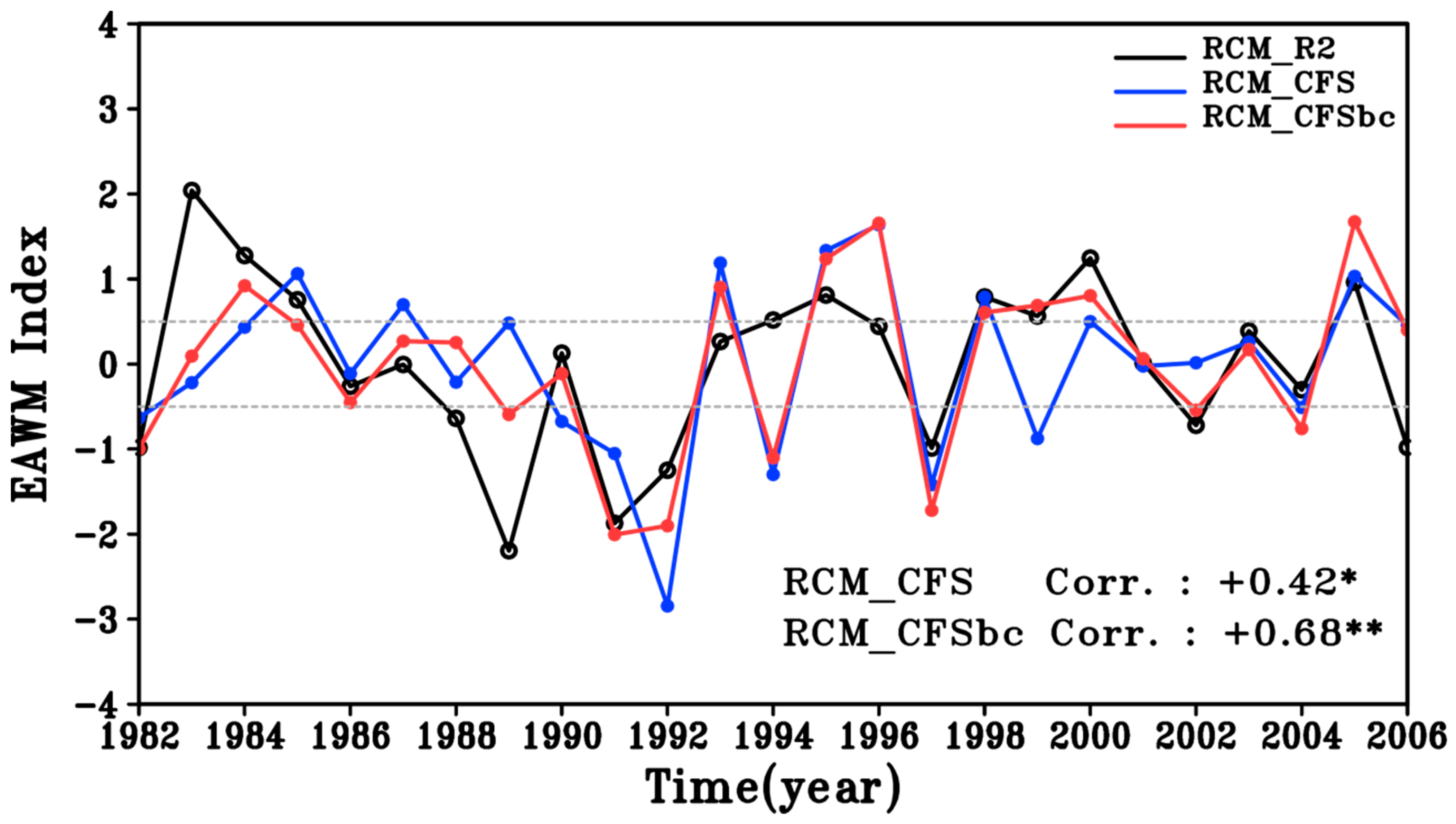
In order to examine the performance skill of the RCM simulation in inter-annual perspective, we calculate the EAWM index proposed by Li and Yang [56], which is calculated as the horizontal rate of change of the 200 hPa zonal wind (Figure 7). A standard deviation of 0.5 is used to select the strong and weak EAWM cases. The EAWM indices calculated from the RCM_R2 experiment had high values in 1983, 1984, 1985, 1995, 2000, and 2005, and low values in 1982, 1989, 1991, 1992, 1997, and 2006. The RCM_CFS captures inter-annual variations well, however it predicts an opposite sign in 1983, 1989, 1994, and 1999. The RCM_CFSbc follows the RCM_R2 simulation more realistically in most years, with a correlation coefficient of 0.68 exceeding the 99% confidence level. In the following, a composite analysis is performed to assess the simulated component of EAWM associated with this index.
Figure 8 shows the composite difference between the strong monsoon years (1983, 1984, 1985, 1995, 2000, 2005) and the weak monsoon years (1982, 1989, 1991, 1992, 1997, 2006) based on the RCM_R2 simulation. In strong monsoon years, the Siberian high (Aleutian low) is stronger (weaker) than that in the weak monsoon years (Figure 8a). This represents the typical pressure pattern for the East Asian winter season where the pressure is high in the west and low in the east. This feature is relatively weak in the CFS-driven experiments, however, when the bias-corrected CFS forecast data are prescribed, it can be observed that the 95% confidence area for the weakening of the Aleutian low-pressure is wider (Figure 8b,c). The spatial pattern of the composite difference for the upper-level geopotential height is similar to the MSLP (Figure 8d). The RCM_CFS simulates this feature weakly, but the RCM_CFSbc represents higher reliability with 95% confidence levels than the RCM_CFS (Figure 8e,f). A strong EAWM is associated with a lower temperature over the north of 20° N (Figure 8g). The 2 m temperature in strong monsoon years is lower than that in weak monsoon years over Korea, China, and Japan. This is due to the expansion of the Siberian high with cold air from high latitudes, which appears in strong monsoon years. Although two CFS-driven experiments can simulate these features (Figure 8h,i), no significance was observed. This is related to underestimation of the Siberian high in strong monsoon years. In the case of the upper jet, it shows a waveform shape (Figure 8j), which indicates that the East Asian jet stream strengthens in strong monsoon years, and is accompanied by an increase in the easterlies over the tropics and a decrease in the westerlies over the high latitudes. A significant improvement is observed in the RCM_CFSbc in terms of magnitude and location of the upper-level jet (Figure 8l).
Generally, the application of a bias-corrected GCM to an RCM results in an improved simulation. The improvement appears to be more remarkable in the case of the tropics and mid-latitudes than in high-latitudes. One possible reason for this is that the CFS hindcast fails to reproduce the high sea level pressure and geopotential height at the 500 hPa level over the Ural Mountains and the anomalous easterlies over the Asian continent [26,28,57]. In the CFS hindcast, the differences in the Siberian high, East Asian jet stream, and the northerlies over East Asia between strong and weak EAWM years are overall weaker than the observations.
3.3. Extreme Event
In order to investigate the effect of bias correction on a climate phenomenon that has a shorter time scale than its seasonal scale, we analyzed the cold surge, which has a great influence on the East Asian winter. The cold surge is a rapid decline in temperature over 1–2 days, and its definition varies by region and nation. Cold surges in East Asia are caused by the strengthening of the Siberian high and a sudden drop in surface air temperature [58]. Park et al. [59] defined the occurrence of cold surges based on the methodology of Zhang et al. [58] and Jeong and Ho [60] as follows: the intensity of the Siberian high is greater than 1 standard deviation, and the daily mean temperature drop of three consecutive days should be greater than −1.5 standard deviation of the winter climatology. Also, the daily temperature should be below the mean winter temperature as it must be a cold day. In this section, we attempted a trial application of bias correction for the wintertime of 2005/06, when East Asia underwent an extraordinarily cold period for approximately one month. Given the definition, three cold surges occurred in the winter of 2005/06: 2 December 2005, 2 January 2006, and 1 February 2006 [59]. In this section, we examine the effect of the GCM bias correction on the simulation of a cold surge event by investigating the case of 2 December 2005.
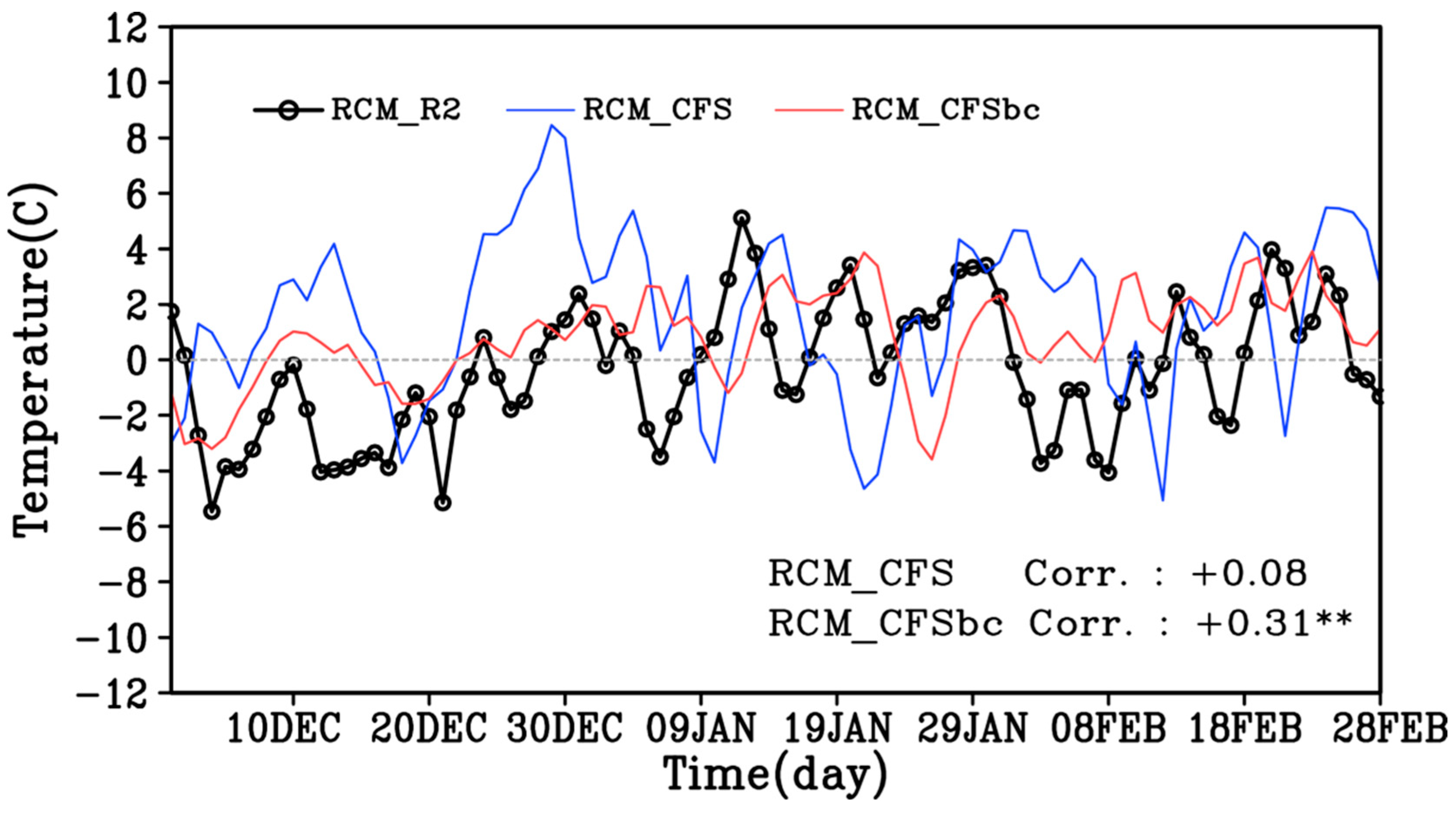
Figure 9 shows the time series of the daily 2 m temperature anomalies in East Asia during the winter of 2005. The first cold surge occurred on 2 December. Considering a typical period of a cold surge, 5–14 days [58], this cold weather was extraordinarily prolonged. The simulated temperatures in the experiment with non-corrected CFS data as the boundary condition are higher than those of the RCM_R2 during December 2005. In particular, the simulated temperature in early December 2005, when the cold surge started, increases gradually. However, in the experiment where the bias-corrected CFS data were used, the temperature variations are relatively similar to those of the RCM_R2 experiment.
In order to examine the temperature distribution during the cold surges in December 2005, we analyzed the surface temperature anomalies of 2–5 December (Figure 10). The RCM_R2 shows strong positive anomalies in the north-eastern Asian regions including Russia during cold surge event, and negative anomalies in other regions (Figure 10a). In contrast, the RCM_CFS simulates negative anomalies in the north-eastern regions, and positive anomalies in Mongolia (Figure 10b). In contrast, the RCM_CFSbc shows strong positive anomalies in north-eastern Asia and negative anomalies in Mongolia, which indicates an improved pattern as compared to that of the RCM_CFS experiment (Figure 10c).
In order to identify the cause of this difference, the evolution of the upper-level geopotential was analyzed. Figure 11 shows the anomalies of the geopotential height at 300 hPa during ±1 day relative to the cold surge on 2 December 2005. The day before the cold surges, 1 December, strong anomalies were formed near the Sea of Okhotsk (Figure 11a). These positive anomalies moved southwestward from 1 to 3 December, and were reminiscent of anomaly patterns generated in artic regions and descended slowly at a high-latitude [61,62,63]. The strong anomalies in the upper-level troposphere and negative anomalies in the mid-latitude formed a dipole pattern in the north-south direction. The RCM_CFS experiment does not show a dipole pattern because the positive anomalies located in the northern region are weakly simulated and the negative anomalies are located over the Korean peninsula (Figure 11b). The RCM_CFSbc, in contrast, clearly shows a dipole pattern similar to that of the RCM_R2. Furthermore, the positive anomalies are shown to move westward in contrast to the RCM_CFS experiment.
In order to examine the vertical structure of the upper-level and lower-level circulation fields, we analyzed the vertical distribution of the geopotential height (Figure 12). Figure 12a shows positive anomalies in the high-latitudes and negative anomalies in the mid-latitudes. On the day of the cold surge, the positive anomalies appear stronger and continue until the next day, which indicates a strong barotropic atmosphere structure of upper-level blocking. Strong positive anomalies above 50° N cause an anticyclonic circulation at the surface, thus allowing the Siberian high to expand to East Asia. According to Takaya and Nakamura [64], a vertically strong coupling causes cold advection in the lower-level, which expands the anticyclonic circulation at the surface. In the RCM_CFS experiment, negative anomalies are dominant up to 60° N, and positive anomalies do not expand to the surface (Figure 12b). As a result, RCM_CFS weakly simulates the Siberian high, thus reducing the inflow of cold air to East Asia. In the experiment with bias correction, the positive anomalies are slightly underestimated, but a nearly barotropic structure of upper-level blocking (Figure 12c).
The results show that the experiment with the corrected GCM simulates a more realistic cold surge event that occurred in December 2005. This suggests that the application of the bias correction method improves the simulation of upper-level circulation and its modulating effect in amplifying the Siberian high to induce the cold surge in East Asia.
4. Summary and Conclusions
We investigated the effect of bias correction on the simulated climate over East Asia using an RCM. Three sets of simulations with different initial and boundary data were conducted for 25 winters from 1982 to 2006. Two GCM-driven experiments were compared with a reanalysis-driven experiment to validate the performance. The comparison shows that the experiment with the use of bias correction results in an improved pattern of temperature, geopotential height, and wind. These improvements were significant in the mid-troposphere owing to the application of a spectral nudging technique. The spectral nudging method used in this study comprises the application of a vertically weighted damping coefficient to reduce the nudging strength in the low level, which may result in a weaker impact of bias correction at low levels.
The experiment with bias correction showed an improved performance in reproducing the spatial distribution as well as interannual variability. Furthermore, the RCM_CFSbc follows the RCM_R2 more realistically in terms of simulating the EAWM. When we use the bias-corrected GCM, the differences between strong and weak monsoon years were more significant. However, the impact of the bias correction method in simulating a high pressure over mid-latitudes was modest, which is related to the inaccuracies of the GCM boundary condition. This implies that the performance of dynamical downscaling is still sensitive to the boundary condition although the bias correction method is able to improve the regional climate simulation in terms of climatological means and inter-annual variability.
The effect of the bias correction on the simulation of extreme events was evaluated. The RCM_CFSbc produced a more realistic temperature distribution for the cold surge event that occurred on 2 December 2005. This is owing to better agreement of the circulations with the results from the reanalysis-driven experiment. However, the bias correction cannot faithfully predict the observed decline in surface temperature. The limitation of this study is that the effect of bias correction on a simulated extreme event cannot be satisfactorily determined because only one case study was performed. Nevertheless, the modest impact implies that the correction to the external forcing works positively to reduce errors and improve dynamical downscaling. It should also be noted that no increased skill would be gained by dynamical downscaling if the variability in the synoptic scale is not resolved in the larger model or reanalysis [65].
This study suggests that the application of a bias correction to the GCM boundary conditions for a regional climate model may be suitable for many regional climate simulations. A correction to the mean bias of the GCM forecast plays a role in improving the major biases that can cause serious issues for regional climate simulations. The presented method is effective in eliminating errors in large-scale circulations rather than local circulations. In other words, the application of bias correction may not promise improved skill in reproducing the fields caused by local instabilities such as precipitation. Therefore, a future investigation is necessary to assess the contribution of the bias correction techniques in improving the simulation of precipitation variability with greater accuracy.
Author Contributions
Conceptualization, Y.-B. Yhang, and S. Ham; methodology, C.-M. Lim, and Y.-B. Yhang; validation, C.-M. Lim.; writing—original draft preparation, C.-M. Lim, Y.-B. Yhang, and S. Ham; writing—review and editing, Y.-B. Yhang, C.-M. Lim, and S. Ham; visualization, C.-M. Lim.
Funding
This research received no external funding.
Acknowledgments
This research was supported by the APEC Climate Center. The APEC Climate Center operations are supported by KREONET (Korea Research Environment Open NETwork) which is managed and operated by KISTI (Korea Institute of Science and Technology Information).
Conflicts of Interest
The authors declare no conflict of interest.
References
- Molteni, F.; Buizza, R.; Palmer, T.N.; Petroliagis, T. The ECMWF Ensemble Prediction System: Methodology and validation. Q. J. R. Meteorol. Soc. 1996, 122, 73–119. [Google Scholar] [CrossRef]
- Saha, S.; Moorthi, S.; Wu, X.; Wang, J.; Nadiga, S.; Tripp, P.; Behringer, D.; Hou, Y.-T.; Chuang, H.; Iredell, M.; et al. The NCEP Climate Forecast System Version 2. J. Clim. 2013, 27, 2185–2208. [Google Scholar] [CrossRef]
- MacLachlan, C.; Arribas, A.; Peterson, K.A.; Maidens, A.; Fereday, D.; Scaife, A.A.; Gordon, M.; Vellinga, M.; Williams, A.; Comer, R.E.; et al. Global Seasonal forecast system version 5 (GloSea5): A high-resolution seasonal forecast system. Q. J. R. Meteorol. Soc. 2015, 141, 1072–1084. [Google Scholar] [CrossRef]
- Giorgi, F.; Bates, G.T. The climatological skill of a regional model over complex terrain. Mon. Weather Rev. 1989, 117, 2325–2347. [Google Scholar] [CrossRef]
- Hong, S.-Y.; Kanamitsu, M. Dynamical downscaling: Fundamental issues from an NWP point of view and recommendations. Asia-Pac. J. Atmos. Sci. 2014, 50, 83–104. [Google Scholar] [CrossRef]
- Zhu, C.; Pierce, D.W.; Barnett, T.P.; Wood, A.W.; Lettenmaier, D.P. Evaluation of hydrologically relevant PCM climate variables and large-scale variability over the continental U.S. Clim. Chang. 2004, 62, 45–74. [Google Scholar] [CrossRef]
- Yoon, J.-H.; Ruby Leung, L.; Correia, J. Comparison of dynamically and statistically downscaled seasonal climate forecasts for the cold season over the United States. J. Geophys. Res. Atmos. 2012, 117. [Google Scholar] [CrossRef]
- Lee, J.-W.; Hong, S.-Y.; Chang, E.-C.; Suh, M.-S.; Kang, H.-S. Assessment of future climate change over East Asia due to the RCP scenarios downscaled by GRIMs-RMP. Clim. Dyn. 2014, 42, 733–747. [Google Scholar] [CrossRef]
- Ham, S.; Lee, J.-W.; Yoshimura, K. Assessing future climate changes in the East Asian summer and winter monsoon using Regional Spectral Model. J. Meteorol. Soc. Jpn. Ser. II 2016, 94A, 69–87. [Google Scholar] [CrossRef]
- Castro, C.L.; Pielke Sr, R.A.; Leoncini, G. Dynamical downscaling: Assessment of value retained and added using the Regional Atmospheric Modeling System (RAMS). J. Geophys. Res Atmos. 2005, 110. [Google Scholar] [CrossRef]
- Xue, Y.; Janjic, Z.; Dudhia, J.; Vasic, R.; De Sales, F. A review on regional dynamical downscaling in intraseasonal to seasonal simulation/prediction and major factors that affect downscaling ability. Atmos. Res. 2014, 147, 68–85. [Google Scholar] [CrossRef]
- Liao, Z.; Zhang, Y. Simulation of a persistent snow storm over Southern China with a regional atmosphere-ocean coupled model. Adv. Atmos. Res. 2013, 30, 425–447. [Google Scholar] [CrossRef]
- Solmoan, S.A.; Pessacg, N.L. Evaluating uncertainties in regional climate simulations over South America at the seasonal scale. Clim. Dyn. 2012, 39, 59–76. [Google Scholar] [CrossRef]
- Mearns, L.O.; Arritt, R.W.; Biner, S.; Bukovsky, M.; McGinnis, S.; Sain, S.; Caya, D.; Correia, J., Jr.; Flori, D.; Gutowski, W.J.; et al. The NorthAmerican Regional Climate Change Assessment Program: Overview of phase I results. Bull. Am. Meteorol. Soc. 2012, 93, 1337–1362. [Google Scholar] [CrossRef]
- Sato, T.; Kimura, F.; Kitoh, A. Projection of global warming onto regional precipitation over Mongolia using a regional climate model. J. Hydrol. 2007, 333, 144–154. [Google Scholar] [CrossRef]
- Hoffmann, P.; Katzfey, J.J.; McGregor, J.L.; Thatcher, M. Bias and variance correction of sea surface temperatures used for dynamical downscaling. J. Geophys. Res. Atmos. 2016, 121, 12–877. [Google Scholar] [CrossRef]
- Rocheta, E.; Evans, J.P.; Sharma, A. Can bias correction of regional climate model lateral boundary conditions improve low-frequency rainfall variability? J. Clim. 2017, 30, 9785–9806. [Google Scholar] [CrossRef]
- Dai, A.; Rasmussen, R.M.; Ikeda, K.; Liu, C. A new approach to construct representative future forcing data for dynamic downscaling. Clim. Dyn. 2017. [Google Scholar] [CrossRef]
- Xu, Z.; Yang, Z.-L. A new dynamical downscaling approach with GCM bias corrections and spectral nudging. J. Geophys. Res. Atmos. 2015, 120, 3063–3084. [Google Scholar] [CrossRef]
- Meyer, J.D.D.; Jin, J. Bias correction of the CCSM4 for improved regional climate modeling of the North American monsoon. Clim. Dyn. 2016, 46, 2961–2976. [Google Scholar] [CrossRef]
- Ramzan, M.; Ham, S.; Amjad, M.; Chang, E.-C.; Yoshimura, K. Sensitivity Evaluation of Spectral Nudging Schemes in Historical Dynamical Downscaling for South Asia. Adv. Meteorol. 2017. [Google Scholar] [CrossRef]
- Chang, C.-P.; Lau, K.-M. Northeasterly cold surges and near-equatorial disturbances over the winter MONEX area during December 1974. Part 2: Planetary-scale aspects. Mon. Weather Rev. 1980, 108, 298–312. [Google Scholar] [CrossRef]
- Lau, K.-M.; Chang, C.-P. Monsoon Meteorology; Oxford University Press: Oxford, UK, 1987; pp. 161–201. [Google Scholar]
- Hong, S.-Y.; Yhang, Y.-B. Implications of a Decadal Climate Shift over East Asia in Winter: A Modeling Study. J. Clim. 2010, 23, 4989–5001. [Google Scholar] [CrossRef]
- Sohn, S.-J.; Tam, C.-Y.; Park, C.-K. Leading modes of East Asian winter climate variability and their predictability: An assessment of the APCC Multi-Model Ensemble. J. Meteorol. Soc. Jpn. 2011, 89, 455–474. [Google Scholar] [CrossRef]
- Jiang, X.; Yang, S.; Li, Y.; Kumar, A.; Wang, W.; Gao, Z. Dynamical prediction of the East Asian winter monsoon by the NCEP Climate Forecast System. J. Geophys. Res. Atmos. 2013, 118, 1312–1328. [Google Scholar] [CrossRef]
- Wang, L.; Chen, W. An intensity index for the East Asian winter monsoon. J. Clim. 2013, 27, 2361–2374. [Google Scholar] [CrossRef]
- Kang, D.; Lee, M.-I. ENSO influence on the dynamical seasonal prediction of the East Asian Winter Monsoon. Clim. Dyn. 2017. [Google Scholar] [CrossRef]
- Seth, A.; Rojas, M. Simulation and sensitivity in a nested modeling study for South America. Part I: Reanalysis boundary forcing. J. Clim. 2003, 6, 2437–2453. [Google Scholar] [CrossRef]
- Lo, J.C.; Yang, Z.-L.; Pielke, R.A., Sr. Assessment of three dynamical climate downscaling methods using the Weather Research and Forecasting (WRF) model. J. Geophys. Res. 2008, 113, D09112. [Google Scholar] [CrossRef]
- Kanamitsu, M.; Yoshimura, K.; Yhang, Y.-B.; Hong, S.-Y. Errors of interannual variability and trend in dynamical downscaling of reanalysis. J. Geophys. Res. 2010, 115, D17115. [Google Scholar] [CrossRef]
- Ainslie, B.; Jackson, P.L. Downscaling and bias correcting a cold season precipitation climatology over coastal couthern British Columbia using the regional atmospheric modeling system (RAMS). J. Appl. Meteorol. Climatol. 2010, 49, 937–953. [Google Scholar] [CrossRef]
- Heikkila, U.; Sandvik, A.; Sorteberg, A. Dynamical downscaling of ERA-40 in complex terrain using the WRF regional climate model. Clim. Dyn. 2010, 37, 1551–1564. [Google Scholar] [CrossRef] [Green Version]
- Misra, V.; Kanamitsu, M. Anomaly nesting: A methodology to downscale seasonal climate simulations from AGCM. J. Clim. 2004, 17, 3249–3262. [Google Scholar] [CrossRef]
- Katzfey, J.J.; McGregor, J.L.; Nguyen, K.C.; Thatcher, M. Dynamical Downscaling Techniques: Impact on Regional Climate Change Signals. In Proceedings of the World IMACS/MODSIM Congress, Cairns, Australia, 13–17 July 2009; pp. 2377–2383. [Google Scholar]
- Hong, S.-Y.; Park, H.; Cheong, H.-B.; Kim, J.-E.E.; Koo, M.-S.; Jang, J.; Ham, S.; Hwang, S.-O.; Park, B.-K.; Chang, E.-C.; et al. The Global/Regional Integrated Model system (GRIMs). Asia-Pac. J. Atmos. Sci. 2013, 49, 219–243. [Google Scholar] [CrossRef]
- Juang, H.H.; Hong, S.-Y.; Kanamitsu, M. The NCEP Regional Spectral Model: An update. Bull. Am. Meteorol. Soc. 1997, 78, 2125–2144. [Google Scholar] [CrossRef]
- Yhang, Y.-B.; Hong, S.-Y. Improved physical processes in a regional climate model and their impact on the simulated summer monsoon circulations over East Asia. J. Clim. 2008, 21, 963–979. [Google Scholar] [CrossRef]
- Yhang, Y.-B.; Hong, S.-Y. A simulated climatology of the East Asian summer monsoon using a regional spectral model. Asia-Pac. J. Atmos. Sci. 2008, 44, 325–339. [Google Scholar]
- Yhang, Y.-B.; Sohn, S.-J.; Jung, I.-W. Application of Dynamical and Statistical Downscaling to East Asian Summer Precipitation for Finely Resolved. Adv. Meteorol. 2017. [Google Scholar] [CrossRef]
- Lee, J.-W.; Ham, S.; Hong, S.-Y.; Yoshimura, K.; Joh, M. Future Changes in Surface Runoff over Korea Projected by a Regional Climate Model under A1B Scenario. Adv. Meteorol. 2014. [Google Scholar] [CrossRef]
- Lee, J.-W.; Hong, S.-Y. Potential for added value to downscaled climate extremes over Korea by increased resolution of a regional climate model. Theor. Appl. Climatol. 2014, 117, 667–677. [Google Scholar] [CrossRef]
- Hong, S.-Y.; Pan, H.-L. Convective trigger function for a mass-flux cumulus parameterization scheme. Mon. Weather Rev. 1998, 126, 2599–2620. [Google Scholar] [CrossRef]
- Byun, Y.-H.; Hong, S.-Y. Improvements in the subgrid-scale representation of moist convection in a cumulus parameterization scheme: The single-column test and its impact on seasonal prediction. Mon. Weather Rev. 2007, 135, 2135–2154. [Google Scholar] [CrossRef]
- Chou, M.-D.; Lee, K.-T.; Tsay, S.-C.; Fu, Q. Parameterization for cloud longwave scattering for use in atmospheric models. J. Clim. 1999, 12, 159–169. [Google Scholar] [CrossRef]
- Chou, M.-D.; Lee, K.-T. A parameterization of the effective layer emission for infrared radiation calculations. J. Atmos. Sci. 2005, 62, 531–541. [Google Scholar] [CrossRef]
- Chou, M.-D.; Suarez, M.J. A solar radiation parameterization (CLIRAD-SW) for atmospheric studies. NASA Tech. Memo 1999, 10460, 48. [Google Scholar]
- Chen, F.; Dudhia, J. Coupling an advanced land surface–hydrology model with the Penn State–NCAR MM5 modeling system. Part I: Model implementation and sensitivity. Mon. Weather Rev. 2001, 129, 569–585. [Google Scholar] [CrossRef]
- Hong, S.-Y.; Noh, Y.; Dudhia, J. A new vertical diffusion package with an explicit treatment of entrainment processes. Mon. Weather Rev. 2006, 134, 2318–2341. [Google Scholar] [CrossRef]
- Hong, S.-Y.; Jang, J. Impacts of shallow convection processes on a simulated boreal summer cliatmology in a global atmospheric model. Asia-Pac. J. Atmos. Sci. 2018, 54, 361–370. [Google Scholar] [CrossRef]
- Hong, S.-Y.; Juang, H.-M.H.; Zhao, Q. Implementation of Prognostic Cloud Scheme for a Regional Spectral Model. Mon. Weather Rev. 1998, 126, 2621–2639. [Google Scholar] [CrossRef]
- Ham, S.; Hong, S.-Y.; Byun, Y.-H.; Kim, J. Effects of precipitation physics algorithms on a simulated climate in a general circulation model. J. Atmos. Sol. Terr. Phys. 2009, 71, 1924–1934. [Google Scholar] [CrossRef]
- Hong, S.-Y.; Chang, E.-C. Spectral nudging sensitivity experiments in a regional climate model. Asia-Pac. J. Atmos. Sci. 2012, 48, 345–355. [Google Scholar] [CrossRef]
- Kanamitsu, M.; Ebisuzaki, W.; Woollen, J.; Yang, S.; Hnilo, J.J.; Fiorino, M.; Potter, G.L. NCEP-DOE AMIP-II reanalysis (R-2). Bull. Am. Meteorol. Soc. 2002, 83, 1631–1644. [Google Scholar] [CrossRef]
- Saha, S.; Nadiga, S.; Thiaw, C.; Wang, J.; Wang, W.; Zhang, Q.; Van den Dool, H.M.; Pan, H.-L.; Moorthi, S.; Behringer, D.; et al. The NCEP Climate Forecast System. J. Clim. 2006, 19, 3483–3517. [Google Scholar] [CrossRef] [Green Version]
- Li, Y.; Yang, S. A dynamical index for the East Asian winter monsoon. J. Clim. 2010, 23, 4255–4262. [Google Scholar] [CrossRef]
- Kim, H.M.; Webster, P.J.; Curry, J. A Seasonal prediction skill of ECMWF System 4 and NCEP CFSv2 retrospective forecast for the Northern Hemisphere Winter. Clim. Dyn. 2012, 12, 2957–2973. [Google Scholar] [CrossRef]
- Zhang, Y.; Sperber, K.R.; Boyle, J.S. Climatology and interannual variation of the East Asian winter monsoon: Results from the 1979-95 NCEP/NCAR reanalysis. Mon. Weather Rev. 1997, 125, 2605–2619. [Google Scholar] [CrossRef]
- Park, T.-W.; Jeong, J.-H.; Ho, C.-H.; Kim, S.-J. Characteristics of atmospheric circulation associated with cold surge occurrences in East Asia: A case study during 2005/06 winter. Adv. Atmos. Sci. 2008, 25, 791–804. [Google Scholar] [CrossRef]
- Jeong, J.-H.; Ho, C.-H. Changes in occurrence of cold surges over east Asian in association with Arctic Oscillation. Geophy. Res. Lett. 2005, 32, L14704. [Google Scholar] [CrossRef]
- Branstator, G. Astriking example of the atmosphere’s leading traveling pattern. J. Atmos. Sci. 1987, 44, 2310–2323. [Google Scholar] [CrossRef]
- Kushnir, Y. Retrograding wintertime low-frequency disturbance over the North Pacific Ocean. J. Atmos. Sci. 1987, 44, 2727–2742. [Google Scholar] [CrossRef]
- Lau, H.-S.; Nath, M.J. Observed and GCM-simulated westward-propagating, planetary-scale fluctuations with approximately three-week periods. Mon. Weather Rev. 1999, 127, 2324–2345. [Google Scholar] [CrossRef]
- Takaya, K.; Nakamura, H. Geographical dependence of upper-level blocking formation associated with intraseasonal amplification of the Siberian high. J. Amos. Sci. 2005, 62, 4441–4449. [Google Scholar] [CrossRef]
- Rockel, B.; Castro, C.L.; Pielke, R.A., Sr; von Storch, H.; Leoncini, G. Dynamical downscaling: Assessment of model system dependent retained and added variability for two different regional climate models. J. Geophys. Res. Atmos. 2008, 113, D21107. [Google Scholar] [CrossRef]
Figure 1.
Regional model (GRIMs) domain. Contour and shading represent the terrain height (m).

Figure 2.
Climatological (1982–2006) December–January–February (DJF) mean field (reanalysis-driven (RCM_R2), left) and difference between reanalysis-driven (RCM_R2) and RCM_CFS (RCM_CFS–RCM_R2, center), RCM_CFSbc (RCM_CFSbc–RCM_R2, right) for (a–c) mean sea level pressure (hPa; shaded) and 850 hPa wind (m/s; vector), (d–f) 2 m temperature (K), (g–i) 500 hPa geopotential height (gpm), and (j–l) 200 hPa wind magnitude (m/s).

Figure 3.
Root mean square difference (RMSD) between RCM_R2 and RCM_CFS (blue line), RCM_CFSbc (red line) experiment for (a) temperature (℃), (b) geopotential height (gpm), (c) zonal wind (m/s), and (d) meridional wind (m/s).
Figure 3.
Root mean square difference (RMSD) between RCM_R2 and RCM_CFS (blue line), RCM_CFSbc (red line) experiment for (a) temperature (℃), (b) geopotential height (gpm), (c) zonal wind (m/s), and (d) meridional wind (m/s).

Figure 4.
Time series of DJF mean and temporal correlation coefficient between RCM_R2 (black line) and RCM_CFS (blue line), RCM_CFSbc (red line) experiment for (a) 2 m temperature, (b) 500 hPa geopotential height, (c) mean sea level pressure, and (d) 200 hPa zonal wind over Asian region (70° E–162° E, −10° S–68° N) during 1982–2006 (* and ** indicate that correlation coefficient values are statistically significant at the 95% and 99% confidence levels, respectively).

Figure 5.
Temporal correlation of (a,b) 2 m temperature, (c,d) 500 hPa geopotential height, (e,f) mean sea level pressure, and (g,h) 200 hPa zonal wind between RCM_R2 and RCM_CFS (left) and RCM_CFSbc (right) during the 1982–2006 winter season. Stippled areas indicate significance at the 95% confidence level.

Figure 6.
Time series of pattern correlation between RCM_R2 and RCM_CFS (blue line), RCM_CFSbc (red line) experiment for (a) 2 m temperature, (b) 500 hPa geopotential height, (c) mean sea level pressure, and (d) 200 hPa zonal wind.
Figure 6.
Time series of pattern correlation between RCM_R2 and RCM_CFS (blue line), RCM_CFSbc (red line) experiment for (a) 2 m temperature, (b) 500 hPa geopotential height, (c) mean sea level pressure, and (d) 200 hPa zonal wind.

Figure 7.
Normalized East Asian winter monsoon (EAWM) index [56] for the RCM_R2 (black), RCM_CFS (blue), and RCM_CFSbc (red) experiment and correlation coefficient between RCM_R2 and RCM_CFS, RCM_R2 and RCM_CFSbc experiment during 1982–2006. Two gray dashed lines indicate ±0.5σ (* and ** indicate significant at the 95% and 99% confidence levels, respectively).

Figure 8.
Composite difference distribution (strong–weak monsoon years) of the (a–c) mean sea level pressure, (d–f) 500 hPa geopotential height, (g–i) 2 m temperature, and (j–l) 200 hPa wind magnitude for RCM_R2 (left), RCM_CFS (center), and RCM_CFSbc (right) experiments. Stippled areas indicate significance at the 95% confidence levels (positive value is red, and negative value is blue).

Figure 9.
Time series of daily anomaly of 2 m temperature for RCM_R2 (black line), RCM_CFS (blue line), and RCM_CFSbc (red line) experiment during DJF 2005/06 over East Asia (110° E–130° E, 20° N–45° N). Correlation coefficients are also shown at the bottom right in the figure and ** indicates significance at the 99% confidence level.

Figure 10.
Anomaly of 2 m temperature (℃) of (a) RCM_R2, (b) RCM_CFS, and (c) RCM_CFSbc experiment during 2–5 December 2005.
Figure 10.
Anomaly of 2 m temperature (℃) of (a) RCM_R2, (b) RCM_CFS, and (c) RCM_CFSbc experiment during 2–5 December 2005.

Figure 11.
Geopotential height anomaly (gpm) at 300 hPa for (a) RCM_R2, (b) RCM_CFS, and (c) RCM_CFSbc experiment during −1 day to +1 day relative to the cold surge occurrence on 2 December 2005. Contour intervals are 100 m.
Figure 11.
Geopotential height anomaly (gpm) at 300 hPa for (a) RCM_R2, (b) RCM_CFS, and (c) RCM_CFSbc experiment during −1 day to +1 day relative to the cold surge occurrence on 2 December 2005. Contour intervals are 100 m.

Figure 12.
Latitude-pressure cross-section of anomaly of geopotential height (m) averaged over 120° E–140° E for (a) RCM_R2, (b) RCM_CFS, and (c) RCM_CFSbc experiment during −1 day to +1 day relative to the cold surge occurrence on 2 December 2005. Contour intervals are 50 m (solid and dashed lines indicate positive and negative values, respectively).


Table 1.
Global/Regional Integrated Model System (GRIMs) physics packages version 3.2.
| Physical Parameterization | GRIMs Version 3.2 |
|---|---|
| Deep convection | Hong and Pan (1998) [43], Byun and Hong (2007) [44] |
| Radiation | SW: Chou et al. (1999) [45] LW: Chou and Lee (2005) [46], Chou and Suarez (1999) [47] |
| Land surface model | Chen and Dudhia (2001) [48] |
| Planetary bounday layer | Hong et al. (2006) [49] |
| Shallow convection | Hong et al. (2012) [50] |
| Microphysics | Hong et al. (1998) [51] |
| Cloudiness | Ham et al. (2009) [52], Hong et al. (1998) [51] |
© 2019 by the authors. Licensee MDPI, Basel, Switzerland. This article is an open access article distributed under the terms and conditions of the Creative Commons Attribution (CC BY) license (http://creativecommons.org/licenses/by/4.0/).
Share and Cite
MDPI and ACS Style
Lim, C.-M.; Yhang, Y.-B.; Ham, S. Application of GCM Bias Correction to RCM Simulations of East Asian Winter Climate. Atmosphere 2019, 10, 382. https://doi.org/10.3390/atmos10070382
AMA Style
Lim C-M, Yhang Y-B, Ham S. Application of GCM Bias Correction to RCM Simulations of East Asian Winter Climate. Atmosphere. 2019; 10(7):382. https://doi.org/10.3390/atmos10070382
Chicago/Turabian StyleLim, Chang-Mook, Yoo-Bin Yhang, and Suryun Ham. 2019. "Application of GCM Bias Correction to RCM Simulations of East Asian Winter Climate" Atmosphere 10, no. 7: 382. https://doi.org/10.3390/atmos10070382
Note that from the first issue of 2016, this journal uses article numbers instead of page numbers. See further details here.