Evaluating Atmospheric Pollutants from Urban Buses under Real-World Conditions: Implications of the Main Public Transport Mode in São Paulo, Brazil

 , and
, and
Abstract
:
1. Introduction
2. Experiments
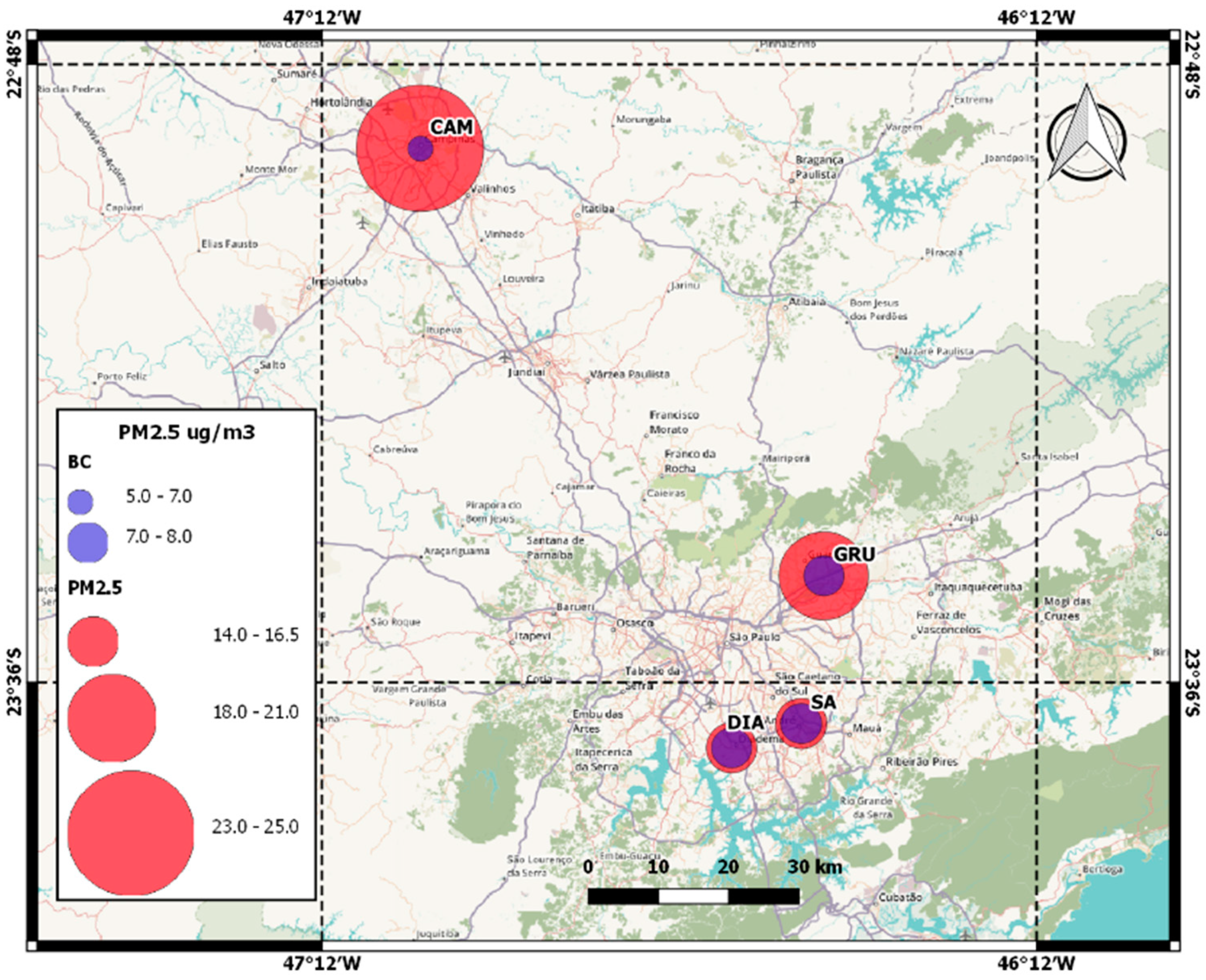
2.1. Sampling Sites
2.2. CO2 and Conventional Gaseous Air Pollutants
2.3. VOC Sampling and Analytical Methods
2.4. PM Sampling and Analytical Methods
2.5. Enrichment Factors
3. Results and Discussion
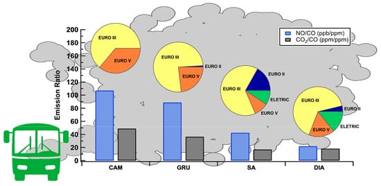
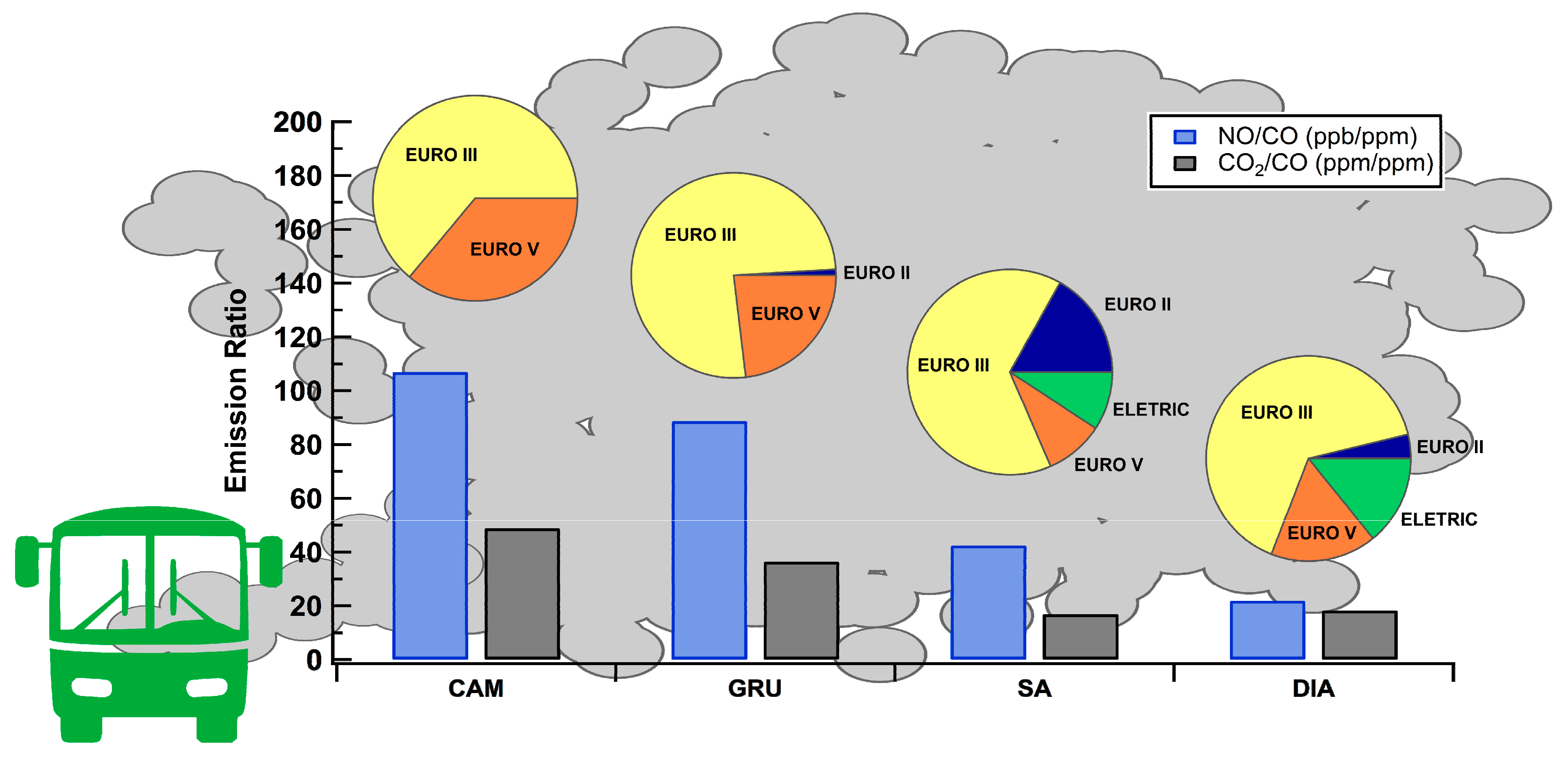
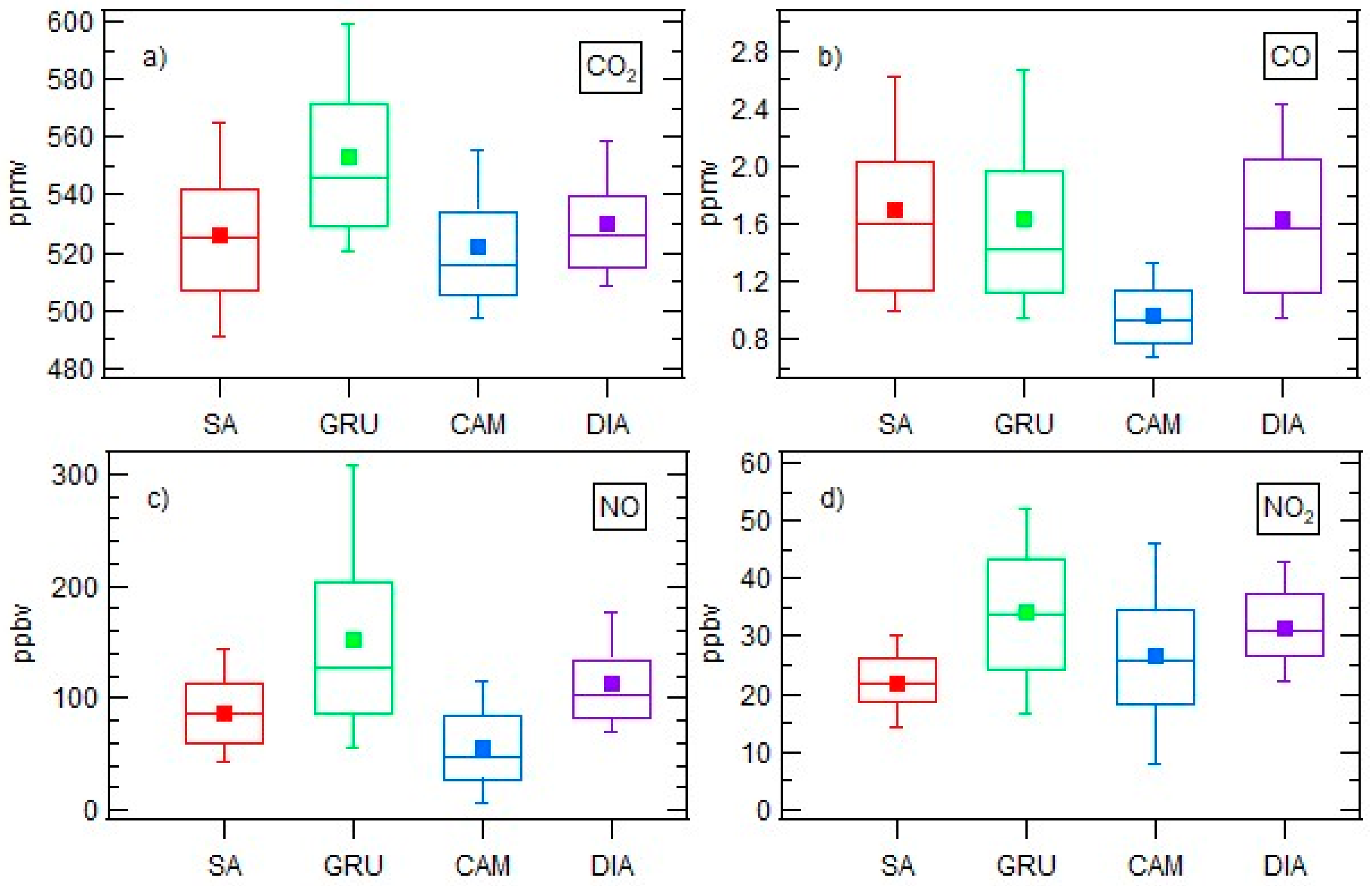
3.1. Regulated Gaseous Pollutants and CO2
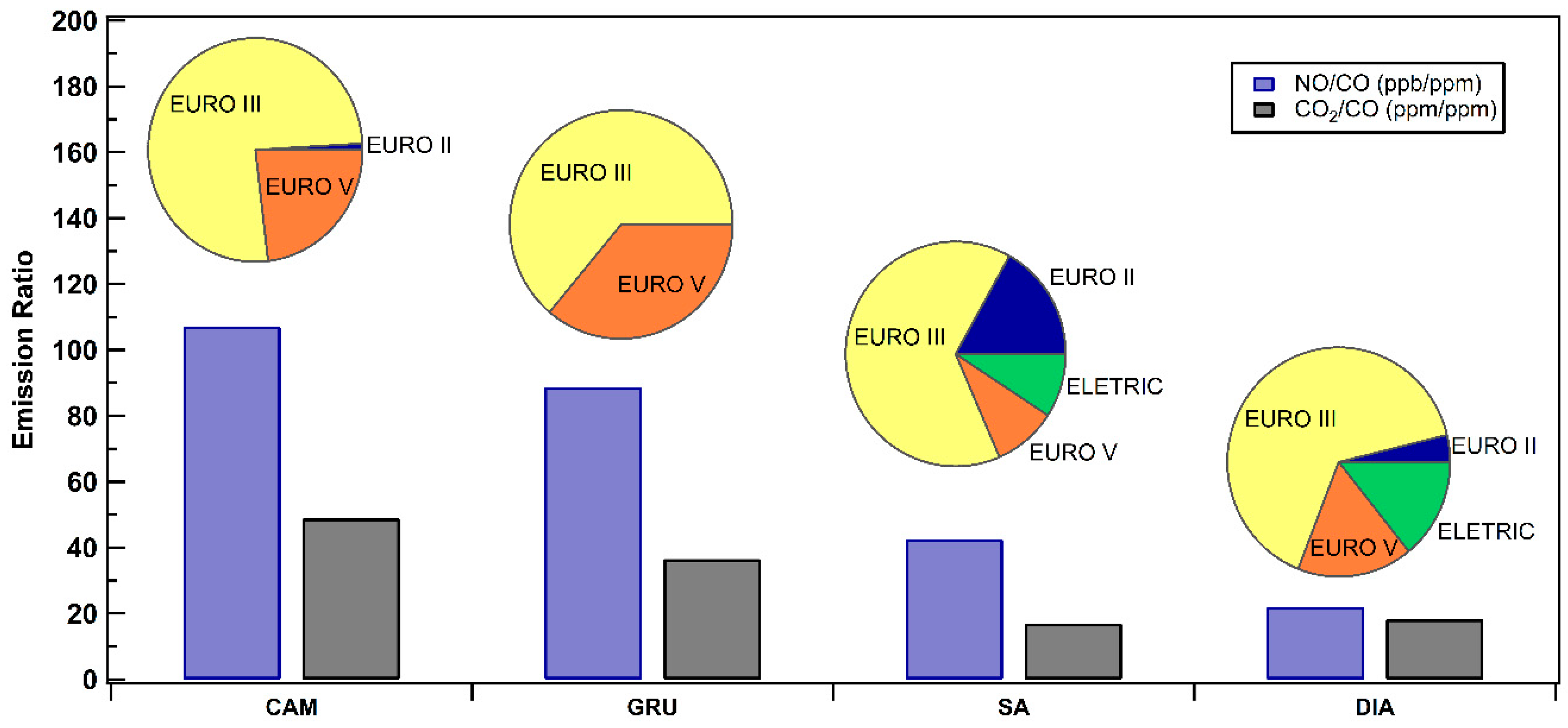
3.2. Emission Reductions and Future Outlook
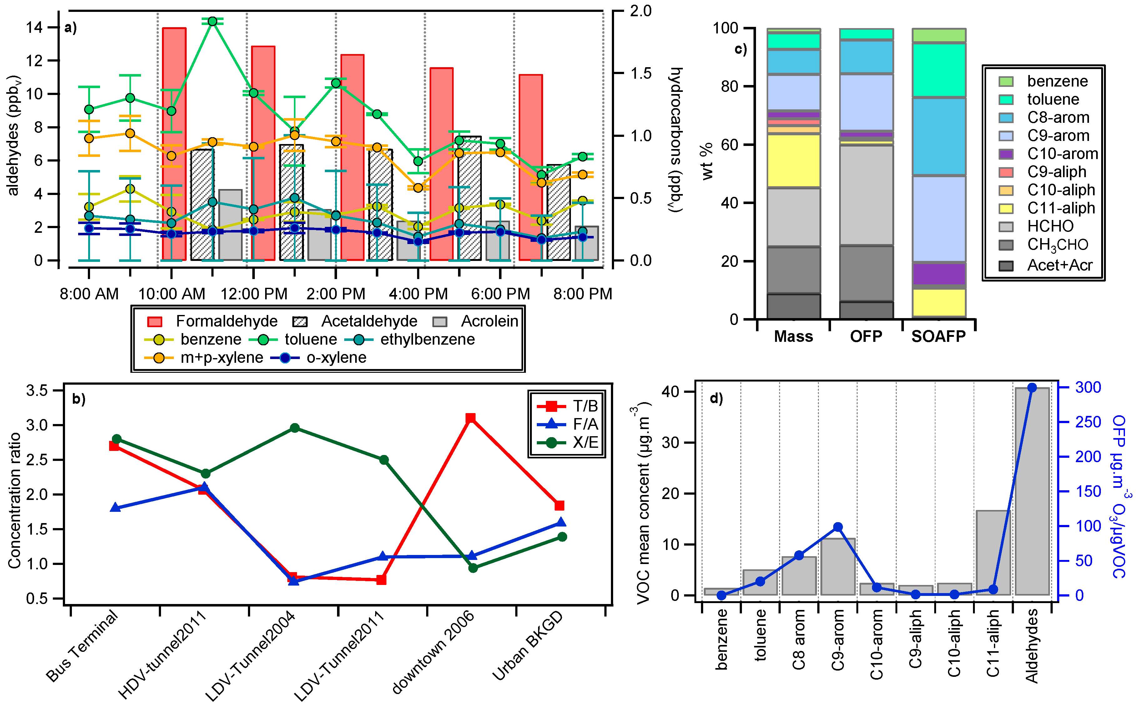
3.3. VOC Measurements
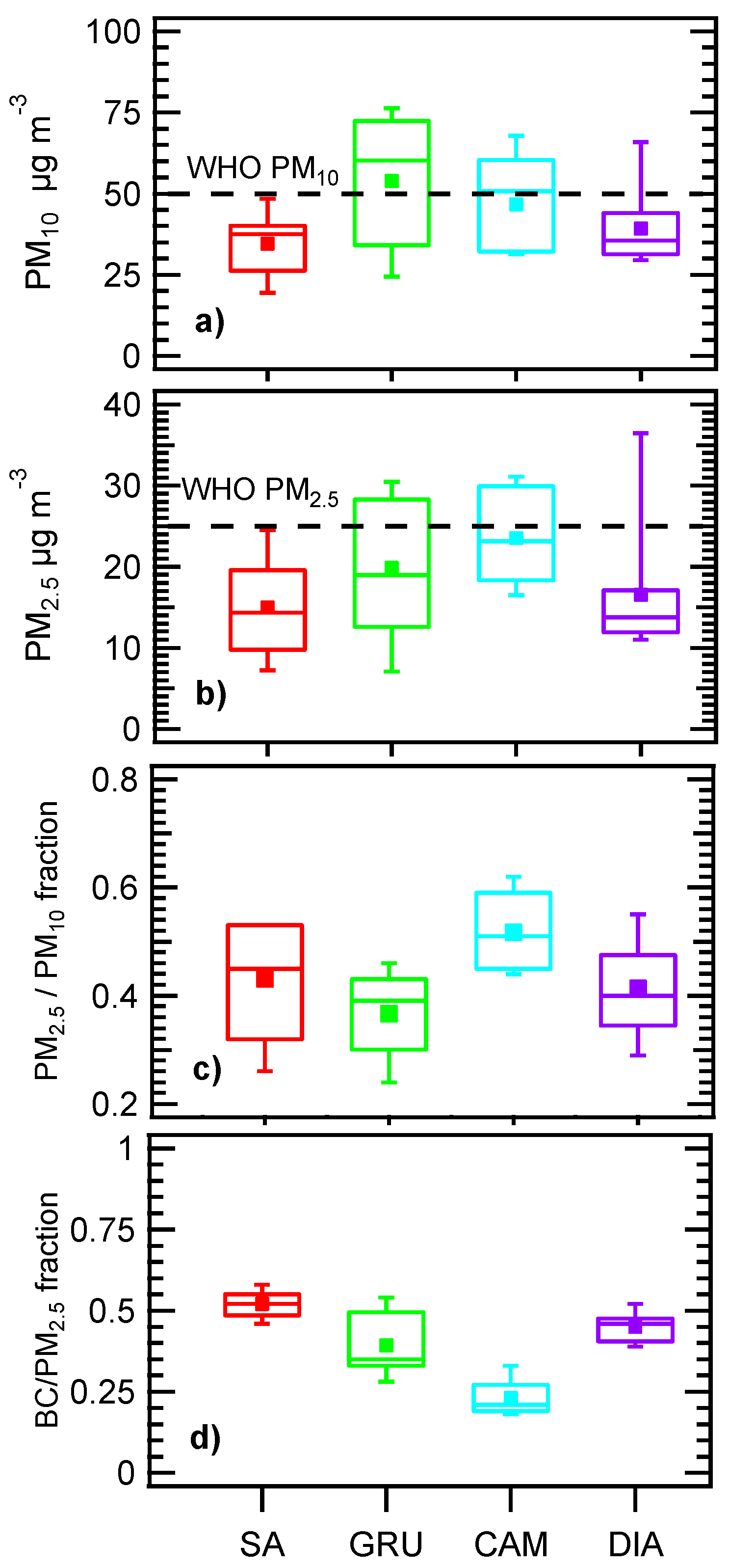
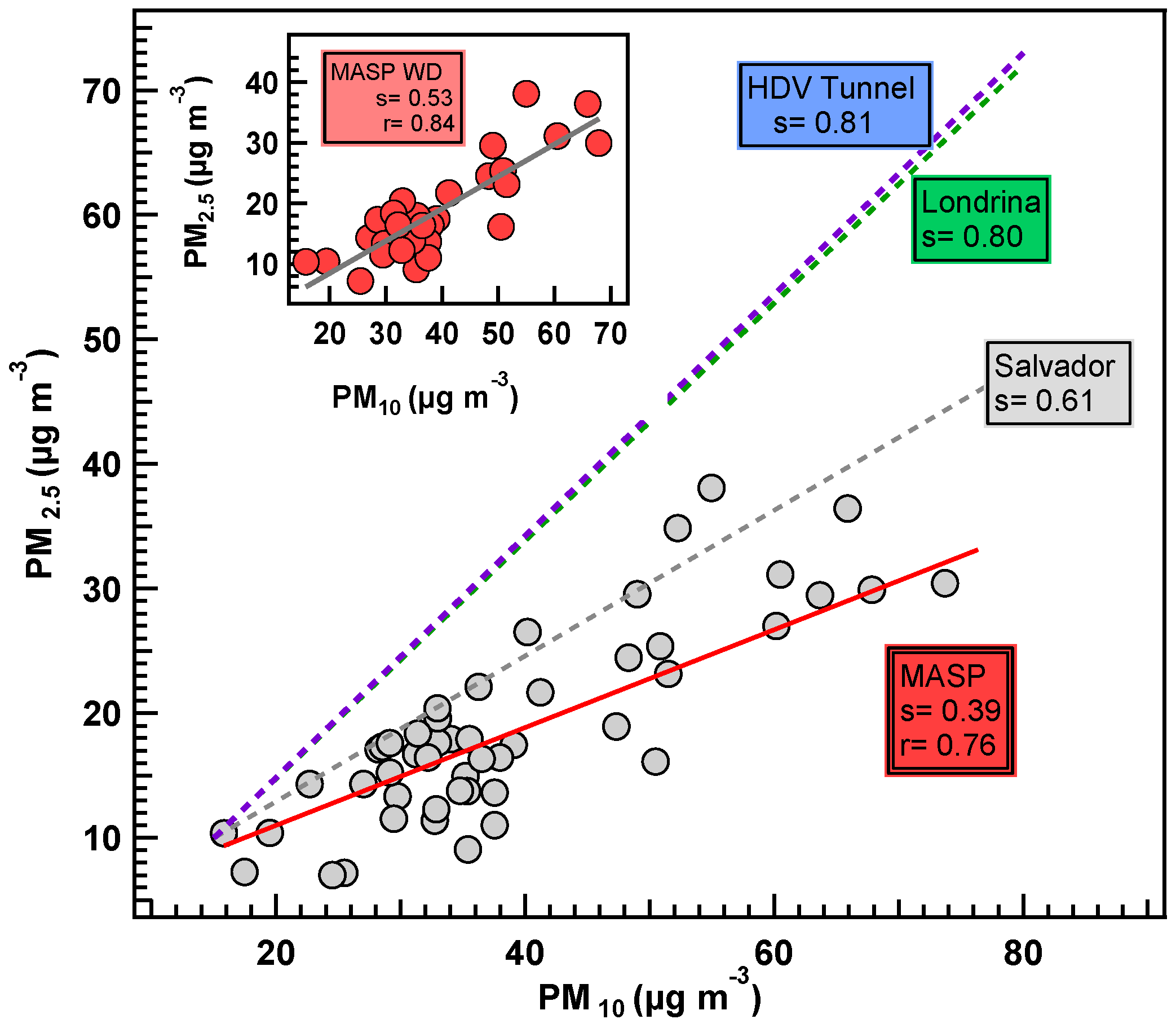
3.4. PM10 and PM2.5 Concentrations
3.5. BC Concentrations
3.6. Source Profile Based on the Mass Balance
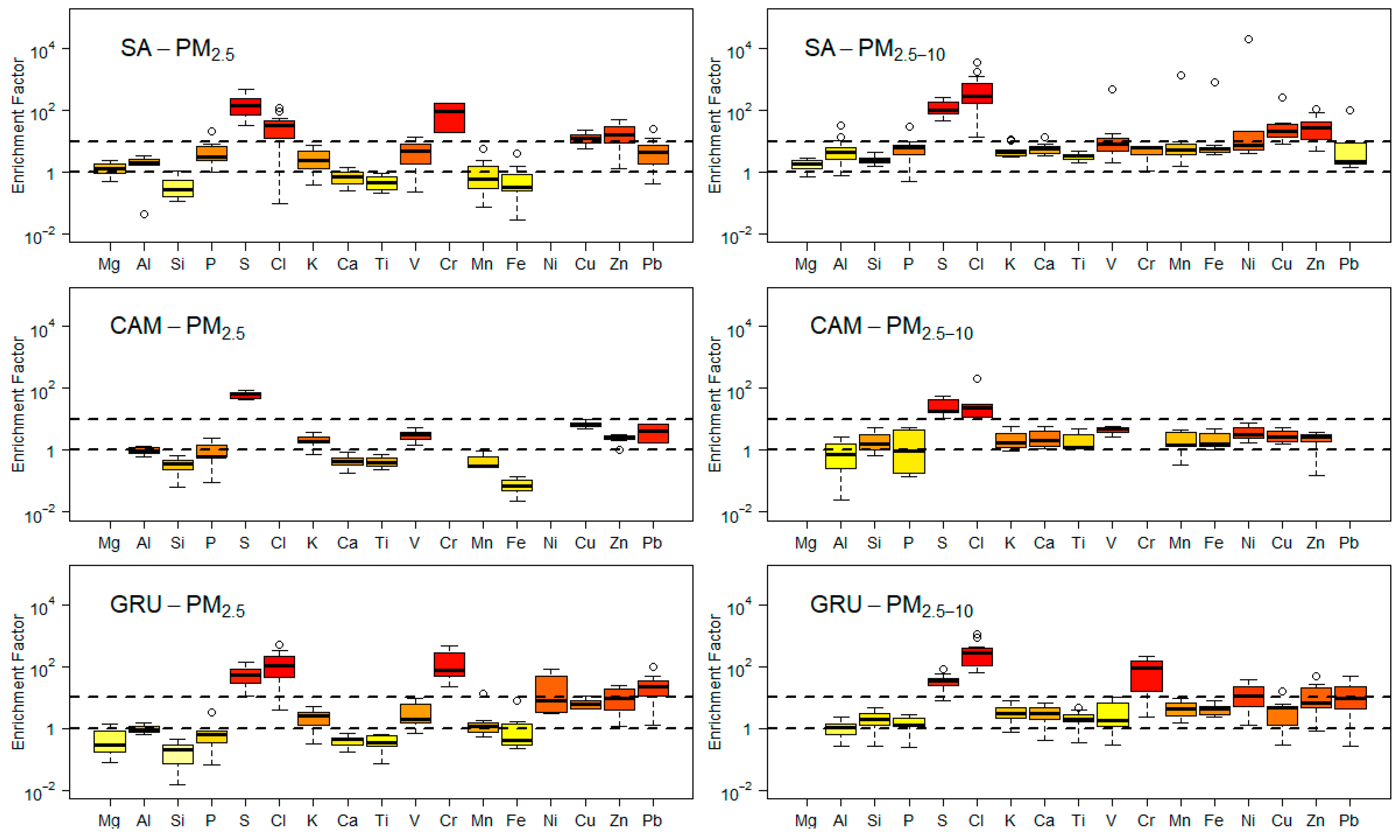
3.7. Enrichment Factors (EFs)
4. Conclusions
Supplementary Materials
Author Contributions
Funding
Acknowledgments
Conflicts of Interest
References
- Landrigan, P.J.; Fuller, R.; Acosta, N.J.R.; Adeyi, O.; Arnold, R.; Basu, N.; Baldé, A.B.; Bertollini, R.; Bose-O’Reilly, S.; Boufford, J.I.; et al. The Lancet Commission on pollution and health. Lancet 2017, 391, 462–512. [Google Scholar] [CrossRef]
- Bravo, M.A.; Son, J.; De Freitas, C.U.; Gouveia, N.; Bell, M.L. Air pollution and mortality in São Paulo, Brazil: Effects of multiple pollutants and analysis of susceptible populations. J. Expos. Sci. Environ. Epidemiol. 2016, 26, 150–161. [Google Scholar] [CrossRef] [PubMed]
- Miranda, R.M.; Andrade, M.F.; Fornaro, A.; Astolfo, R.; de Andre, P.A.; Saldiva, P. Urban air pollution: A representative survey of PM(2.5) mass concentrations in six Brazilian cities. Air Qual. Atmos. Heal. 2012, 5, 63–77. [Google Scholar] [CrossRef] [PubMed]
- Conti, V.; Orchi, S.; Valentini, M.P.; Nigro, M.; Calò, R. Design and evaluation of electric solutions for public transport. Proc. Transp. Res. Procedia 2017, 27, 117–124. [Google Scholar] [CrossRef]
- Cepeda, M.; Schoufour, J.; Freak-Poli, R.; Koolhaas, C.M.; Dhana, K.; Bramer, W.M.; Franco, O.H. Levels of ambient air pollution according to mode of transport: A systematic review. Lancet Public Heal. 2017, 2, e23–e34. [Google Scholar] [CrossRef]
- Lim, S.S.; Vos, T.; Flaxman, A.D.; Danaei, G.; Shibuya, K.; Adair-Rohani, H.; Amann, M.; Anderson, H.R.; Andrews, K.G.; Aryee, M.; et al. A comparative risk assessment of burden of disease and injury attributable to 67 risk factors and risk factor clusters in 21 regions, 1990–2010: A systematic analysis for the Global Burden of Disease Study 2010. Lancet 2012, 380, 2224–2260. [Google Scholar] [CrossRef]
- Pope, C.A.; Dockery, D.W. Health Effects of Fine Particulate Air Pollution: Lines that Connect. J. Air Waste Manag. Assoc. 2006, 56, 709–742. [Google Scholar] [CrossRef] [PubMed] [Green Version]
- Zhang, Q.; Jimenez, J.L.; Canagaratna, M.R.; Ulbrich, I.M.; Ng, N.L.; Worsnop, D.R.; Sun, Y. Understanding atmospheric organic aerosols via factor analysis of aerosol mass spectrometry: A review. Anal. Bioanal. Chem. 2011, 401, 3045–3067. [Google Scholar] [CrossRef] [PubMed]
- Donahue, N.M.; Robinson, A.L.; Pandis, S.N. Atmospheric organic particulate matter: From smoke to secondary organic aerosol. Atmos. Environ. 2009, 43, 94–106. [Google Scholar] [CrossRef]
- UNEP/WHO. Health Effects of Black Carbon; WHO Regional Office for Europe Publications: Copenhagen, Denmark, 2012. [Google Scholar]
- Bond, T.C.; Doherty, S.J.; Fahey, D.W.; Forster, P.M.; Berntsen, T.; Deangelo, B.J.; Flanner, M.G.; Ghan, S.; Kärcher, B.; Koch, D.; et al. Bounding the role of black carbon in the climate system: A scientific assessment. J. Geophys. Res. Atmos. 2013, 118, 5380–5552. [Google Scholar] [CrossRef] [Green Version]
- Jacobson, M.Z. Strong radiative heating due to the mixing state of black carbon in atmospheric aerosols. Nature 2001, 409, 695–697. [Google Scholar] [CrossRef] [PubMed]
- UNEP and Climate and Clean Air Coalition. Short-Lived Climate Pollutants; UNEP and Climate and Clean Air Coalition: Nairobi, Kenya, 2018. [Google Scholar]
- Kumar, P.; Andrade, M.F.; Ynoue, R.Y.; Fornaro, A.; Freitas, E.D.; Martins, J.; Martins, L.D.; Albuquerque, T.; Zhang, Y.; Morawska, L. New directions: From biofuels to wood stoves: The modern and ancient air quality challenges in the megacity of São Paulo. Atmos. Environ. 2016, 140, 364–369. [Google Scholar] [CrossRef] [Green Version]
- IBGE Estimativa da População Residente No Brasil. Diretoria de Pesquisas—Coordenação de População e Indicadores Socias. Available online: https://www.ibge.gov.br/estatisticas-novoportal/sociais/populacao/9103-estimativas-de-populacao.html?=&t=resultados (accessed on 12 February 2019).
- CETESB. Qualidade do ar no estado de São Paulo 2016. Available online: http://ar.cetesb.sp.gov.br/publicacoes-relatorios/ (accessed on 1 January 2018).
- Metro MASP Origen Destination Report. Available online: http://www.metro.sp.gov.br/metro/ arquivos/mobilidade-2012/relatorio-sintese-pesquisa-mobilidade-2012.pdf (accessed on 1 January 2018).
- Pérez-Martínez, P.J.; Andrade, M.F.; Miranda, R.M. Traffic-related air quality trends in São Paulo, Brazil. J. Geophys. Res. Atmos. 2015, 120, 6290–6304. [Google Scholar] [CrossRef] [Green Version]
- Nogueira, T.; Dominutti, P.A.; Fornaro, A.; Andrade, M.F. Seasonal Trends of Formaldehyde and Acetaldehyde in the Megacity of São Paulo. Atmosphere 2017, 8, 144. [Google Scholar] [CrossRef]
- CETESB. Emissões Veiculares no Estado de São Paulo 2016. Available online: http://cetesb.sp.gov.br/veicular/relatorios-e-publicacoes (accessed on 1 January 2018).
- Dominutti, P.A.; Nogueira, T.; Borbon, A.; Andrade, M.F.; Fornaro, A. One-year of NMHCs hourly observations in São Paulo megacity: Meteorological and traffic emissions effects in a large ethanol burning context. Atmos. Environ. 2016, 142, 371–382. [Google Scholar] [CrossRef]
- EPA. Method TO-11A: Compendium of Methods for the Determination of Toxic Organic Compounds in Ambient Air Second Edition Compendium Method TO-11A Determination of Formaldehyde in Ambient Air Using Adsorbent Cartridge Followed by High Performance Liquid Chromat; Center for Environmental Research Information Office of Research and Development U.S. Environmental Protection Agency: Cincinnati, OH, USA, 1999.
- Nogueira, T.; Dominutti, P.A.; Carvalho, L.R.F.; Fornaro, A.; Andrade, M.F. Formaldehyde and acetaldehyde measurements in urban atmosphere impacted by the use of ethanol biofuel: Metropolitan Area of Sao Paulo (MASP), 2012–2013. Fuel 2014, 134, 505–513. [Google Scholar] [CrossRef] [Green Version]
- Hopke, P.K.; Xie, Y.; Raunemaa, T.; Biegalski, S.; Landsberger, S.; Maenhaut, W.; Artaxo, P.; Cohen, D. Characterization of the gent stacked filter unit pm10sampler. Aerosol Sci. Technol. 1997, 27, 726–735. [Google Scholar] [CrossRef]
- Brito, J.; Rizzo, L.V.; Herckes, P.; Vasconcellos, P.C.; Caumo, S.E.S.; Fornaro, A.; Ynoue, R.Y.; Artaxo, P.; Andrade, M.F. Physical–chemical characterisation of the particulate matter inside two road tunnels in the São Paulo Metropolitan Area. Atmos. Chem. Phys. 2013, 13, 12199–12213. [Google Scholar] [CrossRef] [Green Version]
- Gao, Y.; Nelson, E.D.; Field, M.P.; Ding, Q.; Li, H.; Sherrell, R.M.; Gigliotti, C.L.; Van Ry, D.A.; Glenn, T.R.; Eisenreich, S.J. Characterization of atmospheric trace elements on PM2.5 particulate matter over the New York-New Jersey harbor estuary. Atmos. Environ. 2002, 36, 1077–1086. [Google Scholar] [CrossRef]
- IAG Weather Station Bulletin. Available online: http://www.estacao.iag.usp.br (accessed on 2 May 2017).
- Parrish, D.D.; Trainer, M.; Hereid, D.; Williams, E.J.; Olszyna, K.J.; Harley, R.A.; Meagher, J.F.; Fehsenfeld, F.C. Decadal change in carbon monoxide to nitrogen oxide ratio in U.S. vehicular emissions. J. Geophys. Res. 2002, 107, 4140. [Google Scholar] [CrossRef]
- Borbon, A.; Gilman, J.B.; Kuster, W.C.; Grand, N.; Chevaillier, S.; Colomb, A.; Dolgorouky, C.; Gros, V.; Lopez, M.; Sarda-Esteve, R.; et al. Emission ratios of anthropogenic volatile organic compounds in northern mid-latitude megacities: Observations versus emission inventories in Los Angeles and Paris. J. Geophys. Res. Atmos. 2013, 118, 2041–2057. [Google Scholar] [CrossRef] [Green Version]
- ACEA. European Automobile Manufactures Association. Available online: https://www.acea.be/industry-topics/tag/category/euro-standards (accessed on 18 December 2018).
- São Paulo city Lei N° 14.933, de 5 de junho de 2009—Política de Mudança do Clima no Município de São Paulo. Available online: https://leismunicipais.com.br/a/sp/s/sao-paulo/lei-ordinaria/2009/1493/14933/lei-ordinaria-n-14933-2009-institui-a-politica-de-mudanca-do-clima-no-municipio-de-sao-paulo (accessed on 17 December 2018).
- Dunmore, R.E.; Hopkins, J.R.; Lidster, R.T.; Lee, J.D.; Evans, M.J.; Rickard, A.R.; Lewis, A.C.; Hamilton, J.F. Diesel-related hydrocarbons can dominate gas phase reactive carbon in megacities. Atmos. Chem. Phys. 2015, 15, 9983–9996. [Google Scholar] [CrossRef] [Green Version]
- Gentner, D.R.; Isaacman, G.; Worton, D.R.; Chan, A.W.H.; Dallmann, T.R.; Davis, L.; Liu, S.; Day, D.A.; Russell, L.M.; Wilson, K.R.; et al. Elucidating secondary organic aerosol from diesel and gasoline vehicles through detailed characterization of organic carbon emissions. Proc. Natl. Acad. Sci. USA 2012, 109, 18318–18323. [Google Scholar] [CrossRef] [PubMed] [Green Version]
- Gentner, D.R.; Jathar, S.H.; Gordon, T.D.; Bahreini, R.; Day, D.A.; El Haddad, I.; Hayes, P.L.; Pieber, S.M.; Platt, S.M.; de Gouw, J.; et al. Review of Urban Secondary Organic Aerosol Formation from Gasoline and Diesel Motor Vehicle Emissions. Environ. Sci. Technol. 2017, 51, 1074–1093. [Google Scholar] [CrossRef] [PubMed]
- Ait-Helal, W.; Borbon, A.; Sauvage, S.; de Gouw, J.A.; Colomb, A.; Gros, V.; Freutel, F.; Crippa, M.; Afif, C.; Baltensperger, U.; et al. Volatile and intermediate volatility organic compounds in suburban Paris: Variability, origin and importance for SOA formation. Atmos. Chem. Phys. 2014, 14, 10439–10464. [Google Scholar] [CrossRef]
- Do, D.H.; Van Langenhove, H.; Chigbo, S.I.; Amare, A.N.; Demeestere, K.; Walgraeve, C. Exposure to volatile organic compounds: Comparison among different transportation modes. Atmos. Environ. 2014, 94, 53–62. [Google Scholar] [CrossRef]
- Li, S.; Chen, S.; Zhu, L.; Chen, X.; Yao, C.; Shen, X. Concentrations and risk assessment of selected monoaromatic hydrocarbons in buses and bus stations of Hangzhou, China. Sci. Total Environ. 2009, 407, 2004–2011. [Google Scholar] [CrossRef] [PubMed]
- Pinto, J.P.; Solci, M.C. Comparison of rural and urban atmospheric aldehydes in Londrina, Brazil. J. Braz. Chem. Soc. 2007, 18, 928–936. [Google Scholar] [CrossRef] [Green Version]
- Pinto, J.P.; Martins, L.D.; da Silva Junior, C.R.; Sabino, F.C.; Amador, I.R.; Solci, M.C. Carbonyl concentrations from sites affected by emission from different fuels and vehicles. Atmos. Pollut. Res. 2014, 5, 404–410. [Google Scholar] [CrossRef] [Green Version]
- Rodrigues, M.C.; Guarieiro, L.L.N.; Cardoso, M.P.; Souza, L.; Gisele, O.; Andrade, J.B.; Carvalho, L.S.; Da Rocha, G.O.; De Andrade, J.B. Acetaldehyde and formaldehyde concentrations from sites impacted by heavy-duty diesel vehicles and their correlation with the fuel composition: Diesel and diesel/biodiesel blends. Fuel 2012, 92, 258–263. [Google Scholar] [CrossRef] [Green Version]
- Andrade, J.B.; Andrade, M.V.; Pinheiro, H.L.C. Atmospheric Levels of Formaldehyde and Acetaldehyde and their Relationship with the Vehicular Fleet Composition in Salvador, Bahia, Brazil. J. Braz. Chem. Soc. 1998, 9, 219–223. [Google Scholar] [CrossRef]
- Martins, L.D.; Andrade, M.F.; Ynoue, R.Y.; Albuquerque, E.L.; Tomaz, E.; Vasconcellos, P.C. Ambiental volatile organic compounds in the megacity of Sao Paulo. Quim. Nova 2008, 31, 2009–2013. [Google Scholar] [CrossRef]
- Alvim, D.S. Estudo dos Principais Precursores de Ozônio na Região Metropolitana de São Paulo. Ph.D. Thesis, Universidade de São Paulo, São Paulo, Brazil, 2013. [Google Scholar]
- Nogueira, T.; Souza, K.F.; Fornaro, A.; Andrade, M.F.; Carvalho, L.R.F. On-road emissions of carbonyls from vehicles powered by biofuel blends in traffic tunnels in the Metropolitan Area of Sao Paulo, Brazil. Atmos. Environ. 2015, 108, 88–97. [Google Scholar] [CrossRef]
- Bahreini, R.; Middlebrook, A.M.; De Gouw, J.A.; Warneke, C.; Trainer, M.; Brock, C.A.; Stark, H.; Brown, S.S.; Dube, W.P.; Gilman, J.B.; et al. Gasoline emissions dominate over diesel in formation of secondary organic aerosol mass. Geophys. Res. Lett. 2012, 39. [Google Scholar] [CrossRef] [Green Version]
- Hsieh, L.-T.; Yang, H.-H.; Chen, H.-W. Ambient BTEX and MTBE in the neighborhoods of different industrial parks in Southern Taiwan. J. Hazard. Mater. 2006, 128, 106–115. [Google Scholar] [CrossRef] [PubMed]
- Atkinson, R.; Arey, J. Atmospheric Degradation of Volatile Organic Compounds. Chem. Rev. 2003, 103, 4605–4638. [Google Scholar] [CrossRef] [PubMed]
- Monod, A.; Sive, B.C.; Avino, P.; Chen, T.; Blake, D.R.; Sherwood, F.R. Monoaromatic compounds in ambient air of various cities: A focus on correlations between the xylenes and ethylbenzene. Atmos. Environ. 2001, 35, 135–149. [Google Scholar] [CrossRef]
- Giubbina, F.F.; Scaramboni, C.; De Martinis, B.S.; Godoy-Silva, D.; Nogueira, R.F.P.; Campos, M.L.A.M. A simple method for simultaneous determination of acetaldehyde, acetone, methanol, and ethanol in the atmosphere and natural waters. Anal. Methods 2017, 9, 2915–2922. [Google Scholar] [CrossRef]
- Corrêa, S.M.; Arbilla, G. Carbonyl emissions in diesel and biodiesel exhaust. Atmos. Environ. 2008, 42, 769–775. [Google Scholar] [CrossRef]
- Guarieiro, L.L.N.; Pereira, P.A.d.P.; Torres, E.A.; da Rocha, G.O.; de Andrade, J.B. Carbonyl compounds emitted by a diesel engine fuelled with diesel and biodiesel-diesel blends: Sampling optimization and emissions profile. Atmos. Environ. 2008, 42, 8211–8218. [Google Scholar] [CrossRef]
- Guarieiro, L.L.N.; de Souza, A.F.; Torres, E.A.; de Andrade, J.B. Emission profile of 18 carbonyl compounds, CO, CO2, and NOxemitted by a diesel engine fuelled with diesel and ternary blends containing diesel, ethanol and biodiesel or vegetable oils. Atmos. Environ. 2009, 43, 2754–2761. [Google Scholar] [CrossRef]
- Jimenez, J.L.; Canagaratna, M.R.; Donahue, N.M.; Prevot, A.S.; Zhang, Q.; Kroll, J.H.; DeCarlo, P.F.; Allan, J.D.; Coe, H.; Ng, N.L.; et al. Evolution of Organic Aerosols in the Atmosphere: A New Framework Connecting Measurements to Models. Science 2009, 326, 1525–1529. [Google Scholar] [CrossRef] [PubMed]
- Donahue, N.M.; Kroll, J.H.; Pandis, S.N.; Robinson, A.L. A two-dimensional volatility basis set-Part 2: Diagnostics of organic-aerosol evolution. Atmos. Chem. Phys. 2012, 12, 615–634. [Google Scholar] [CrossRef]
- Hamilton, J.F.; Lewis, A.C. Monoaromatic complexity in urban air and gasoline assessed using comprehensive GC and fast GC-TOF/MS. Atmos. Environ. 2003, 37, 589–602. [Google Scholar] [CrossRef]
- Derwent, R.G.; Jenkin, M.E.; Pilling, M.J.; Carter, W.P.L.; Kaduwela, A. Reactivity scales as comparative tools for chemical mechanisms. J. Air Waste Manag. Assoc. 2010, 60, 914–924. [Google Scholar] [CrossRef] [PubMed]
- Gilman, J.B.; Lerner, B.M.; Kuster, W.C.; Goldan, P.D.; Warneke, C.; Veres, P.R.; Roberts, J.M.; De Gouw, J.A.; Burling, I.R.; Yokelson, R.J. Biomass burning emissions and potential air quality impacts of volatile organic compounds and other trace gases from fuels common in the US. Atmos. Chem. Phys. 2015, 15, 13915–13938. [Google Scholar] [CrossRef] [Green Version]
- Carter, W.P.L. Updated Maximum Incremental Reactivity Scale and Hydrocarbon Bin Reactivities for Regulatory Applications. 2010. Available online: https://www.arb.ca.gov/research/reactivity/mir09.pdf (accessed on 15 May 2017).
- WHO. Air Quality Guidelines. Global Update 2005. Particulate Matter, Ozone, Nitrogen Dioxide and Sulfur Dioxide; WHO Regional Office for Europe Publications: Copenhagen, Denmark, 2016. [Google Scholar]
- Andrade, M.F.; Kumar, P.; Freitas, E.D.; Ynoue, R.Y.; Martins, J.; Martins, L.D.; Nogueira, T.; Perez-Martinez, P.; Miranda, R.M.; Albuquerque, T.; et al. Air quality in the megacity of São Paulo: Evolution over the last 30 years and future perspectives. Atmos. Environ. 2017, 159, 66–82. [Google Scholar] [CrossRef] [Green Version]
- Mkoma, S.L.; Da Rocha, G.O.; Regis, A.C.D.; Domingos, J.S.S.; Santos, J.V.S.; De Andrade, S.J.; Carvalho, L.S.; De Andrade, J.B. Major ions in PM2.5 and PM10 released from buses: The use of diesel/biodiesel fuels under real conditions. Fuel 2014, 115, 109–117. [Google Scholar] [CrossRef]
- Martins, L.D.; Silva Junior, C.R.; Solci, M.C.; Pinto, J.P.; Souza, D.Z.; Vasconcellos, P.; Guarieiro, A.L.N.; Guarieiro, L.L.N.; Sousa, E.T.; De Andrade, J.B. Particle emission from heavy-duty engine fuelled with blended diesel and biodiesel. Environ. Monit. Assess. 2012, 184, 2663–2676. [Google Scholar] [CrossRef] [PubMed]
- Pereira, G.M.; Teinilä, K.; Custódio, D.; Gomes Santos, A.; Xian, H.; Hillamo, R.; Alves, C.A.; Andrade, J.B.; Rocha, G.O.; Kumar, P.; et al. Particulate pollutants in the Brazilian city of São Paulo: 1-year investigation for the chemical composition and source apportionment. Atmos. Chem. Phys. 2017, 17, 11943–11969. [Google Scholar] [CrossRef] [Green Version]
- Pérez-Martínez, P.J.; Miranda, R.M.; Nogueira, T.; Guardani, M.L.; Fornaro, A.; Ynoue, R.; Andrade, M.F. Emission factors of air pollutants from vehicles measured inside road tunnels in São Paulo: Case study comparison. Int. J. Environ. Sci. Technol. 2014, 11, 2155–2168. [Google Scholar] [CrossRef]
- Sánchez-Ccoyllo, O.R.; Ynoue, R.Y.; Martins, L.D.; Astolfo, R.; Miranda, R.M.; Freitas, E.D.; Borges, A.S.; Fornaro, A.; Freitas, H.; Moreira, A.; et al. Vehicular particulate matter emissions in road tunnels in Sao Paulo, Brazil. Environ. Monit. Assess. 2009, 149, 241–249. [Google Scholar] [CrossRef] [PubMed]
- Hetem, I.G.; Andrade, M.F. Characterization of fine particulate matter emitted from the resuspension of road and pavement dust in the Metropolitan Area of São Paulo, Brazil. Atmosphere 2016, 7, 31. [Google Scholar] [CrossRef]
- Kumar, A.; Kim, D.-S.; Omidvarbona, H.; Kuppili, S.K. Combustion Chemistry of Biodiesel for Use in Urban Transport Buses: Experiment and Modeling; Mineta National Transit Research Consortium: San Jose, CA, USA, 2014. [Google Scholar]
- Zhang, J.; He, K.; Shi, X.; Zhao, Y. Comparison of particle emissions from an engine operating on biodiesel and petroleum diesel. Fuel 2011, 90, 2089–2097. [Google Scholar] [CrossRef]
- Taylor, S.; McLennan, S. The geochemical evolution of the continental crust. Rev. Geophys. 1995, 33, 241–265. [Google Scholar] [CrossRef]


| Terminal | Sampling Period | Passengers Per Day | Number of Buses on Weekdays/Weekends |
|---|---|---|---|
| SA | May 12–30 | 89,000 | Electric: 330/95 |
| EURO II: 605/400 | |||
| EURO III: 2315/1105 | |||
| EURO V: 332/114 | |||
| GRU | June 3–16 | 39,000 | EURO III: 1380/727 |
| EURO V: 779/412 | |||
| CAM | September 26–October 6 | 70,000 | EURO II: 22/12 |
| EURO III: 1798/982 | |||
| EURO V: 547/288 | |||
| DIA | December 5–19 | 113,000 | Electric: 389/152 |
| EURO II: 104/49 | |||
| EURO III: 1789/802 | |||
| EURO V: 459/204 |
| Parameter | unity | 12–30 May | 3–16 June | 26 Sep–6 Oct | 5–19 Dec |
|---|---|---|---|---|---|
| PM10 | µg m−3 | 23.8 | 32.6 | 22.9 | 23.9 |
| PM2.5 | µg m−3 | 14.1 | 22.3 | 13.7 | 13.7 |
| NO | ppb | 21.4 | 54.9 | 9.6 | 22.1 |
| NO2 | ppb | 16.6 | 24.6 | 12.9 | 21.6 |
| CO | ppm | 0.6 | 1.0 | 0.6 | 0.5 |
| Temperature | °C | 17.3 | 12.7 | 16.7 | 22.0 |
| Rainfall | mm | 150 | 131 | 18 | 57 |
© 2019 by the authors. Licensee MDPI, Basel, Switzerland. This article is an open access article distributed under the terms and conditions of the Creative Commons Attribution (CC BY) license (http://creativecommons.org/licenses/by/4.0/).
Share and Cite
Nogueira, T.; Dominutti, P.A.; Vieira-Filho, M.; Fornaro, A.; Andrade, M.d.F. Evaluating Atmospheric Pollutants from Urban Buses under Real-World Conditions: Implications of the Main Public Transport Mode in São Paulo, Brazil. Atmosphere 2019, 10, 108. https://doi.org/10.3390/atmos10030108
Nogueira T, Dominutti PA, Vieira-Filho M, Fornaro A, Andrade MdF. Evaluating Atmospheric Pollutants from Urban Buses under Real-World Conditions: Implications of the Main Public Transport Mode in São Paulo, Brazil. Atmosphere. 2019; 10(3):108. https://doi.org/10.3390/atmos10030108
Chicago/Turabian StyleNogueira, Thiago, Pamela A. Dominutti, Marcelo Vieira-Filho, Adalgiza Fornaro, and Maria de Fatima Andrade. 2019. "Evaluating Atmospheric Pollutants from Urban Buses under Real-World Conditions: Implications of the Main Public Transport Mode in São Paulo, Brazil" Atmosphere 10, no. 3: 108. https://doi.org/10.3390/atmos10030108