Spatiotemporal Characteristics of the Dominant Modes of Surface Air Temperature Interannual Variations over South China during the Spring-to-Summer Transition

Abstract

The surface air temperature (SAT) interannual variability during the spring-to-summer transition over South China (SC) has been decomposed into two dominant modes by applying empirical orthogonal function (EOF) analysis. The first EOF mode (EOF1) is characterized by homogenous SAT anomalies over SC, whereas the second EOF mode (EOF2) features a dipole SAT anomaly pattern with opposite anomalies south and north of the Yangtze River. A regression analysis of surface heat flux and advection anomalies on the normalized principle component time series corresponding to EOF1 suggests that surface heat flux anomalies can explain SAT anomalies mainly by modulating cloud-shortwave radiation. Negative cloud anomalies result in positive downward shortwave radiation anomalies through the positive shortwave cloud radiation effect, which favor warm SAT anomalies over most of SC. For EOF2, the distribution of advection anomalies resembles the north–south dipole pattern of SAT anomalies. This suggests that wind-induced advection plays an important role in the SAT anomalies of EOF2. Negative SAT anomalies are favored by cold advection from northerly wind anomalies over land surfaces in high-latitude regions. Positive SAT anomalies are induced by warm advection from southerly wind anomalies over the ocean in low-latitude regions.

1. Introduction

Surface air temperature (SAT) variations in South China (SC) play an important role in the local climate, economy, and society. For example, extreme heat wave events affect human health and increase mortality in China [1,2,3]. Low temperatures in summer reduce crop yields at large scales in Northeast China on interannual scale [4,5]. Interannual surface cooling can reduce the East Asian summer monsoon circulation by weakening the land–sea thermal contrast over east China [6,7]. Therefore, it is necessary to investigate SAT interannual variations over SC and their contributing factors to better understand regional climate variability.

Many studies have explored winter SAT anomalies in Asia, and specifically in China. For example, Hu and Liu [8] and Zhuang et al. [9] found that the first empirical orthogonal function (EOF) mode (EOF1) of winter SAT anomalies has a homogeneous structure over Northeast China, and shows a close relationship with the Arctic Oscillation. Kang et al. [10] studied winter temperature variations over China from 1951 to 2000 by EOF analysis, and found that EOF1 is characterized by a homogeneous structure throughout China, whereas the second EOF mode (EOF2) features a dipole pattern with opposite signals over south and north China. Miyazaki and Yasunari [11] clarified the interannual variability in winter SAT over Asia by principal component analysis. They found that SAT variability is strongly affected by atmospheric circulation and sea surface temperatures (SST) anomalies. Xu et al. [12] investigated subseasonal SAT variability during early and late winter over East Asia, and reported that deceleration of the East Asian jet stream in January–February can promote warm SAT anomalies over East Asia.

Many other studies have reported summer SAT anomalies and their contributing factors in East Asia and Northeast China. For example, Wu et al. [13,14,15] studied summer SAT anomalies over Northeast China and demonstrated that the El Niño- Southern Oscillation (ENSO), North Atlantic SST, and spring snow cover are important contributing factors. Chen et al. [16] investigated the interannual variation in summer SAT over Northeast Asia and its associated circulation anomalies. Liang et al. [17] analyzed the subseasonal variability in SAT over East Asia and found that EOF1 and EOF2 correspond to a same-sign SAT anomaly throughout East Asia and an opposite-sign variability over northern and southern East Asia, respectively. These studies have greatly enhanced our understanding of SAT anomalies during winter and summer.

Most previous work has focused on boreal winter or summer. During the spring-to-summer transition, SAT over SC undergoes significant warming because of the northward movement of the area of direct sunlight, and is accompanied by the onset of the South China Sea Summer Monsoon in the middle of May [18,19]. This transition period is distinct from the winter and summer seasons and warrants further investigation. An analysis of this transition period is also expected to improve our understanding of conditions in winter and summer. For example, He and Wu [20] found that SST changes in the southern and central South China Sea (SCS) are affected by cloud-radiation, wind-evaporation, and wind-driven oceanic effects during April–June. Wu and Hu [21] reported that processes during this transition season have important implications for summer precipitation variability over the SCS. Wu and He [22] explored two distinct processes leading to early or late spring-to-summer transitions over the SCS. Studies have also demonstrated the connection between spring-to-summer SAT and the East Asian summer monsoon. He et al. [23] found that during the spring-to-summer transition, the Central South Peninsula, which rapidly increases in temperature and is influenced by the East Asian summer monsoon, is sensitive to the seasonal transition. Zhang [24] reported a periodic rapid increase in temperature over the plateau during the late-spring-to-early-summer transition that is influenced by the East Asian summer monsoon. Yao [25] investigated the interannual changes in SAT and the contribution of surface heat flux to SAT variation in East Asia during the spring-to-summer transition. The results provide a comprehensive picture of spring-to-summer climate variability for some areas, but not for SC SAT. Therefore, an investigation of the factors and processes involved in SC SAT anomalies during the transition season is warranted and is the focus of this work.

In this study, we analyze the dominant modes of SAT interannual variations and the physical processes that influence SAT anomalies. The remainder of the text is organized as follows. Datasets and methods are described in Section 2, and we discuss the spatiotemporal characteristics of SAT interannual variations in Section 3. The processes that contribute to SAT interannual anomalies are analyzed in Section 4. Finally, a summary and discussion are provided in Section 5.

2. Data and Methods

2.1. Datasets

We employed monthly mean SAT data from the Global Historical Climatology Network version 2 and the Climate Anomaly Monitoring System [26] (GHCN-CAMS) for 1948–2017. This dataset has a high horizontal resolution of 0.5° × 0.5° and is available online at https://www.esrl.noaa.gov/psd/data/gridded/data.ghcncams.html. These data have been used in many studies on climate variability [27,28]. We also employed SAT data from the University of Delaware [29] for 1900–2014 on a 0.5° × 0.5° grid to confirm the results obtained from GHCN-CAMS (not shown).

Surface heat flux (sensible heat flux (SH), latent heat flux (LH), shortwave radiation (SWR), and longwave radiation (LWR)), total cloud cover (TCC), and winds and air temperature at 1000 hPa were obtained from the National Centers for Environmental Prediction and the National Center for Atmospheric Research (NCEP/NCAR) reanalysis 1 [30] dataset and are available online at https://www.esrl.noaa.gov/psd/data/gridded/data.ncep.reanalysis.html. Winds and air temperature at 1000 hPa have a horizontal resolution of 2.5° × 2.5°, and surface heat flux and TCC are on a T62 Gaussian grid. The dataset covers the period from 1948 to the present. Monthly mean surface heat fluxes from the Japanese 55-year Reanalysis Project (JRA-55) of the Japan Meteorological Agency [31] were also used to support the analysis of surface heat flux anomalies from the NCEP/NCAR reanalysis 1 dataset.

2.2. Statistical Methods

We used the EOF method to analyze the dominant modes of boreal spring-to-summer SAT interannual variability in SC from 1948 to 2017. The study area extends from 20° to 35° N and from 105° to 125° E, and covers most of SC. The SAT, surface heat flux, and advection anomalies were obtained by simple linear regression on the normalized principle component (PC) time series corresponding to the dominant modes of the SC AMJ (April, May, and June) SAT anomalies during 1948–2017. Area-mean anomalies in surface heat flux and advection, also quantified by simple linear regression, are used to obtain their separate contributions to the SAT variability in selected regions (Figure 1a,b).

2.3. Temperature Equation Diagnosis

Changes in SAT can be caused by many factors. In this work, we employ the thermodynamic equation, showing the main factors affecting the SAT anomalies.

$$\frac{\partial T}{\partial t}+u\frac{\partial T}{\partial x}+v\frac{\partial T}{\partial y}+w\left(\frac{\partial T}{\partial p}-\frac{RT}{C_{p}p}\right)=Q,$$

(1)

where Q is diabatic heating per unit mass, T is SAT, u and v are the horizontal velocity, $w$ is the vertical p-velocity, R is the gas constant, and $C_p$ is the specific heat at constant pressure. The term $u\frac{\partial T}{\partial x}+v\frac{\partial T}{\partial y}$ captures the horizontal advection of temperature and $w\left(\frac{\partial T}{\partial p}-\frac{RT}{C_{p}p}\right)$ captures the vertical heat exchange.

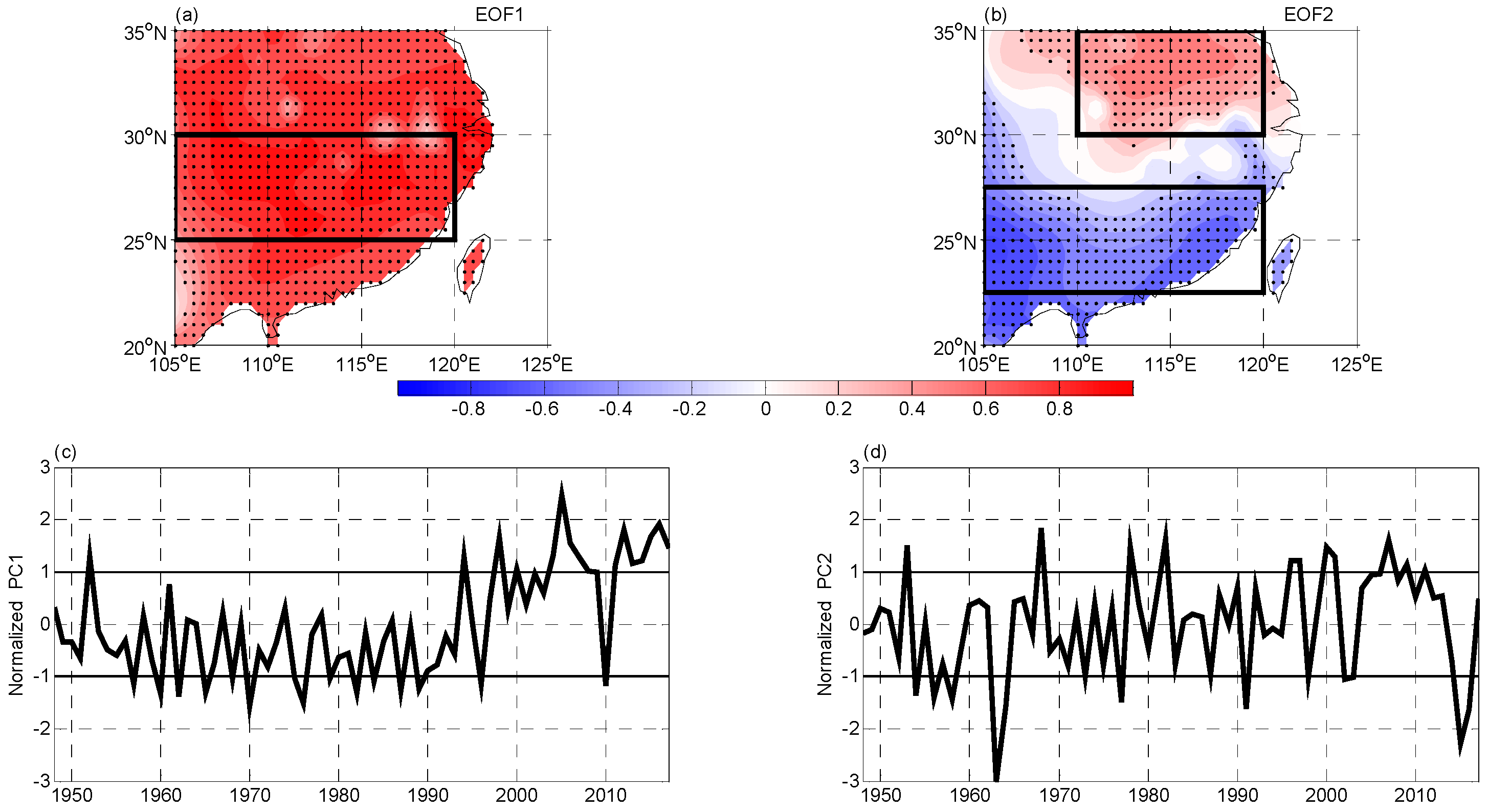
3. Dominant Modes of SAT Anomalies

Figure 1 shows the spatial patterns of SAT interannual anomalies corresponding to EOF1 and EOF2, and their corresponding normalized PC time series (PC1 and PC2, respectively) during 1948–2017. The EOF1 and EOF2 modes explain 64.4% and 14.4% of the total variance, respectively. The first two modes are well separated from the other modes using the method of North et al. [32].

The EOF1 mode was characterized by a same-sign SAT anomaly pattern with significantly strong anomalies (Figure 1a). In the positive phase of EOF1, warm SAT anomalies exceeded 0.8 K in central SC. The largest positive value of PC1 was in 2005 and the largest negative value was in 1970 (Figure 1c). In addition, the PC1 time series underwent a significant decadal shift around 1993 when it changed from a negative to a positive phase (Figure 1c).

The EOF2 mode featured a north–south dipole anomaly pattern with opposite SAT anomalies over north and south of the Yangtze River (~30° N; Figure 1b). During the positive EOF2 phase, there was a significant warm SAT anomaly with a maximum value exceeding 0.6 K centered over the region north of the Yangtze River. Cold SAT anomalies were less than −0.4 K in the east and west of the region south of the Yangtze River. The PC2 time series showed a significantly warmer north and cooler south in 1968, with the opposite pattern in 1963 and 2015 (Figure 1d).

4. Roles of Physical Processes in SAT Anomalies

The atmospheric thermodynamics equation indicates that local temperature changes depend on the horizontal advection of temperature, vertical heat exchange, and diabatic heating. In the near-surface layer, low-level advection and diabatic heating are the primary controls on SAT changes [33,34,35]. Diabatic heating represents the heat exchange between the land and the atmosphere, whereas advection reflects the effects of the heating and cooling processes of atmospheric dynamics. In this section, we discuss the effects of the above two factors on SAT and related physical processes over SC during the spring-to-summer transition period.

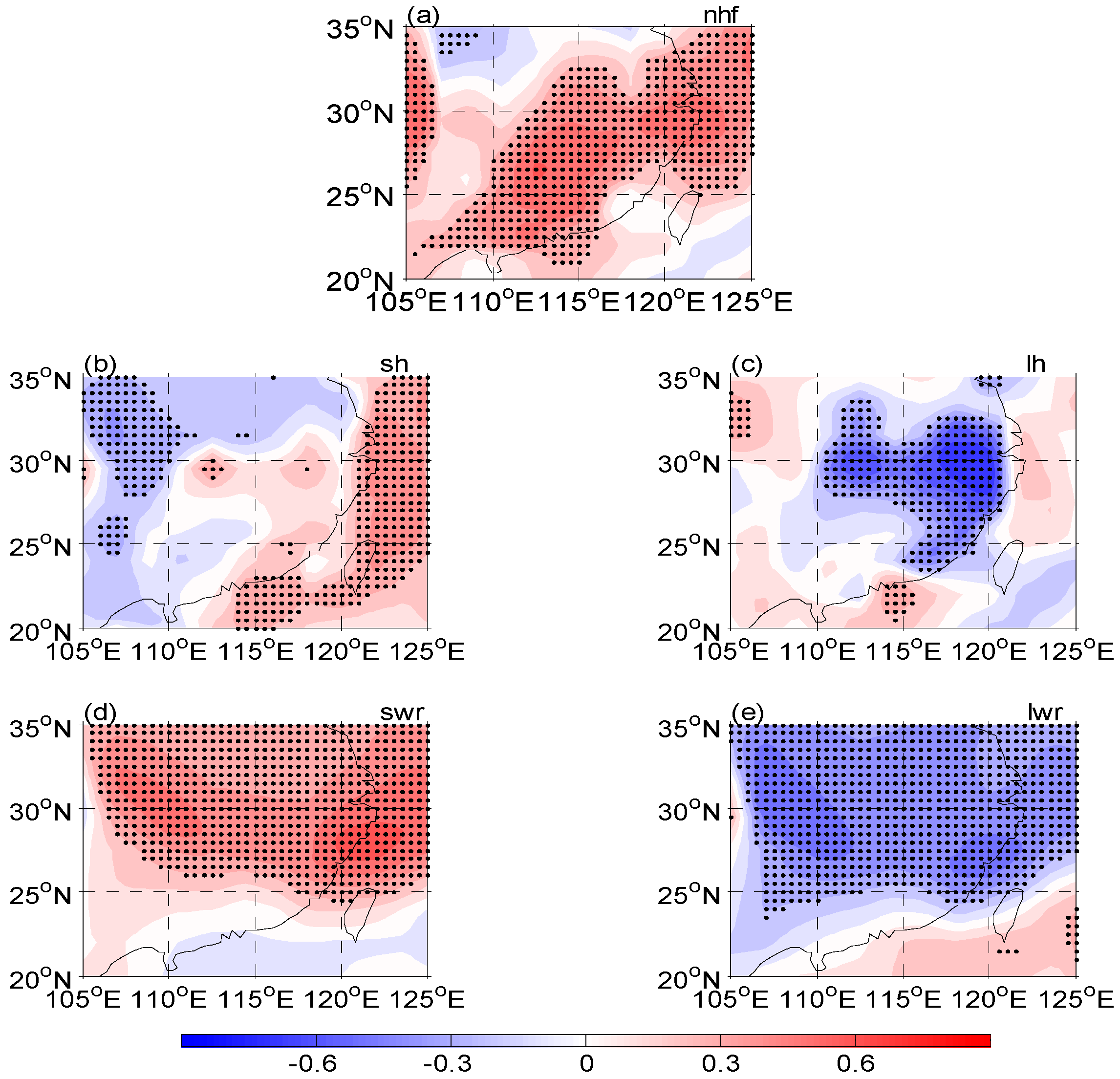
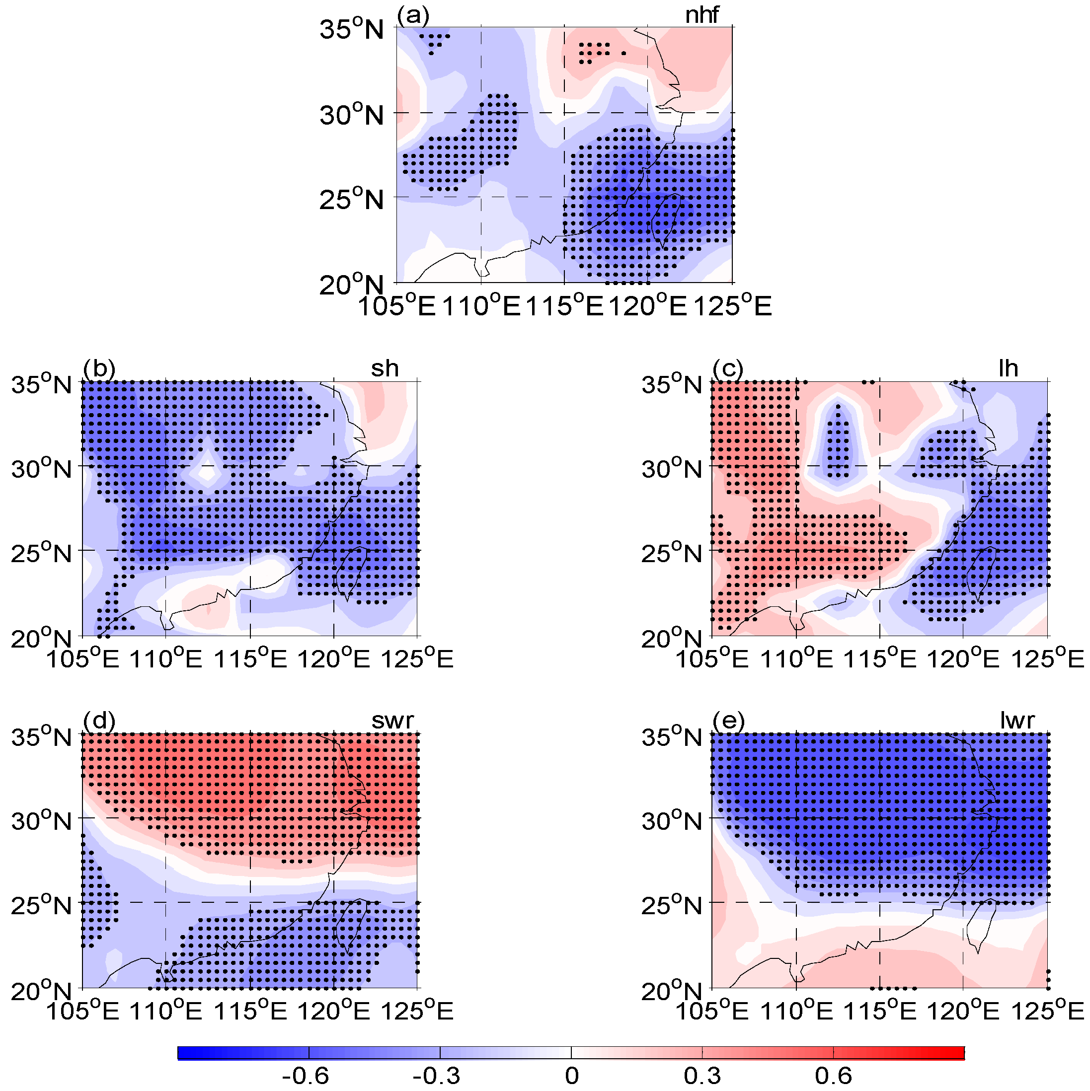
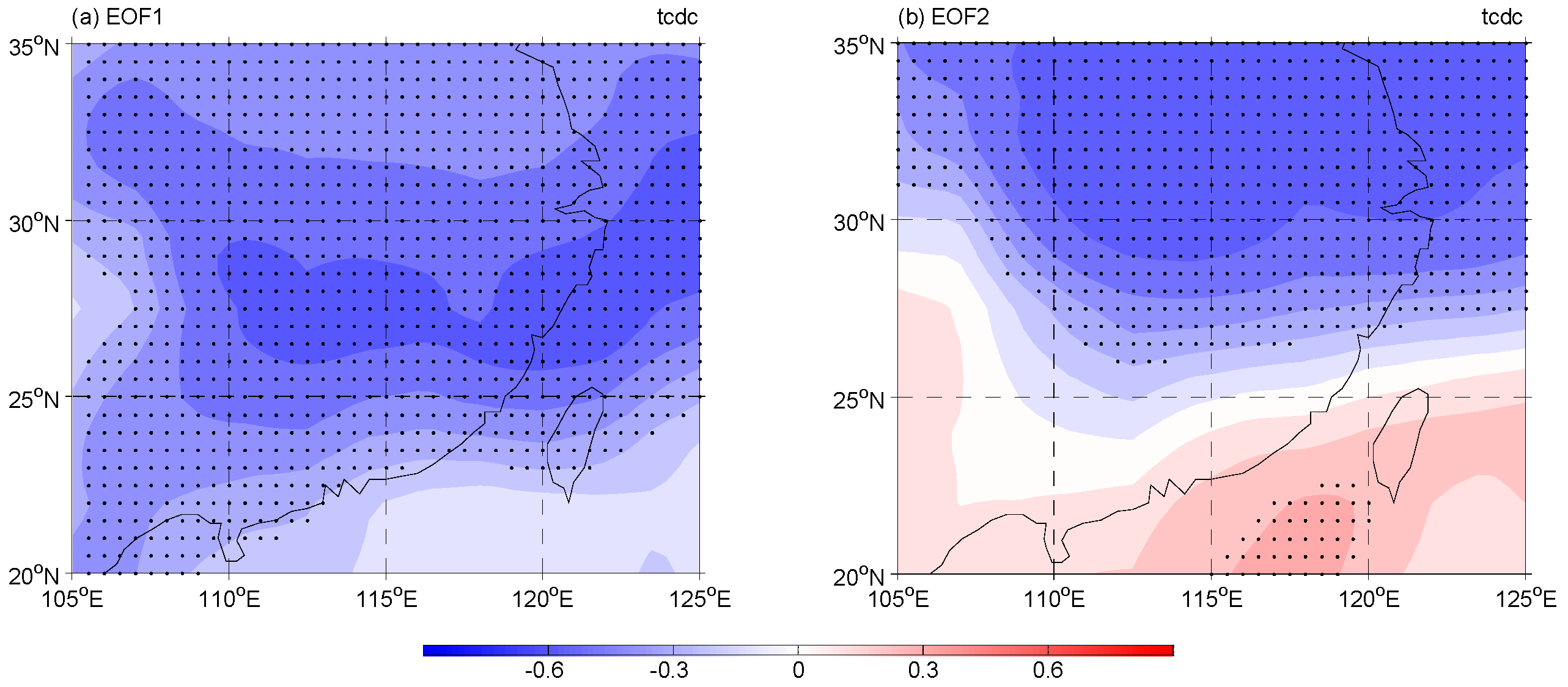
4.1. Surface Heat Flux

SAT variability is closely associated with SH and surface LH variations. Warmer SAT can lead to an increase in upward SH, and LH may indirectly affect SAT anomalies through surface moisture and evapotranspiration effects. More (less) precipitation and vegetation cover accompanied by more (less) surface soil humidity, less (more) cloud cover, and higher (lower) wind speeds may increase (decrease) surface evapotranspiration. This may induce an increase (decrease) in upward surface LH and a decrease (increase) in SAT. SWR and LWR also contribute to changes in SAT; however, the effects of cloud-SWR and cloud-LWR on SAT are different. The cloud–albedo effect predicts that more clouds will reflect more downward SWR. This leads to a decrease in downward SWR that is absorbed by the surface, resulting in a negative SAT anomaly; however, greater upward LWR from the surface will be reflected back to the ground surface when more clouds are present, resulting in a positive SAT anomaly.

Figure 2 and Figure 3 show SH, LH, SWR, LWR, and the net heat flux (NHF) anomalies in AMJ obtained by regression on the normalized PC1 and PC2 of AMJ SAT during 1948–2017. In the following discussion, downward surface heat flux anomalies are defined as positive and represent heat gained by the surface; negative downward flux anomalies correspond to heat lost by the surface.

In EOF1, the NHF (Figure 2a) is significantly positive over most of SC, and the spatial pattern of NHF anomalies is similar to that of SAT anomalies (Figure 1a and Figure 2a). The SH variation (Figure 2b) is positive over areas near 30° N, contributing to the increase in NHF. LH (Figure 2c) makes a large negative contribution to NHF over most of SC. A significant increase in NHF is attributed to net SWR over SC (Figure 2d), and downward SWR makes a large positive contribution to net SWR (not shown). Net LWR (Figure 2e) makes a negative contribution to SAT anomalies over SC. In addition, the spatial pattern of TCC anomalies (Figure 4a) is similar to those of the SWR and LWR anomalies, which indicates that a decrease in cloudiness leads to an increase in downward SWR. Therefore, cloud-SWR processes favor warm SAT in the EOF1 mode over SC.

In EOF2, NHF (Figure 3a) has a dipole structure but differs somewhat from the SAT pattern. NHF is positive only over northeastern areas and is significantly negative over other areas of SC (Figure 3a). The negative NHF is influenced by SH, net SWR, and LWR over south of 30° N (Figure 3a,b,d,e). Net SWR (Figure 3d) makes a large positive contribution to the increase in NHF north of 30° N; however, increased NHF is only present over a small area north of 30° N (northeastern areas) and is caused by decreases in SH, LH, and LWR north of 30° N (Figure 3a–c,e). In addition, the distributions of SWR and LWR (Figure 3d,e) are similar to that of the TCC anomalies (Figure 4b). This suggests that clouds play an important role in SWR and LWR variations.

The above analysis demonstrates that NHF makes an important contribution to the SAT anomalies of EOF1, particularly through cloud-SWR effects. In EOF2, NHF explains SAT changes in only a few areas. A decrease north of 30° N and insignificant anomalies south of 25° N in NHF cannot explain SAT anomalies in these areas (Figure 1b and Figure 3a). Therefore, other factors are likely to have more important effects on the AMJ SAT anomalies of EOF2, and these are discussed in the next subsection.

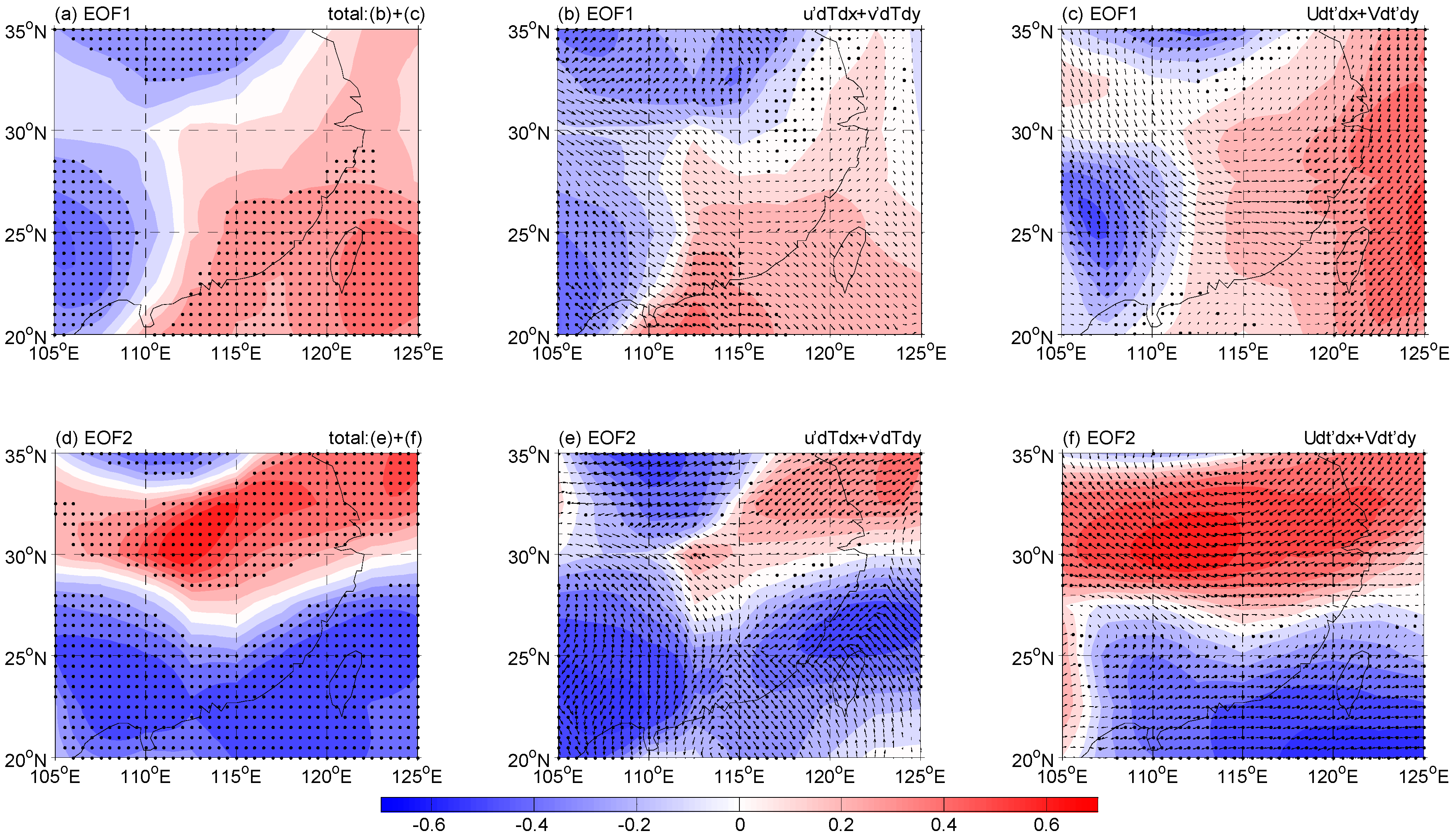
4.2. Advection at 1000 hPa

Advection at 1000 hPa is also an important factor affecting SAT. The temperature advection process can be expressed by four terms: $-u^{\prime }\frac{\partial \overline{T}}{\partial x}$, $-v^{\prime }\frac{\partial \overline{T}}{\partial y}$, $-\overline{u}\frac{\partial T^{\prime }}{\partial x}$, and $-\overline{v}\frac{\partial T^{\prime }}{\partial y}$. The sum of $-u^{\prime }\frac{\partial \overline{T}}{\partial x}$ and $-v^{\prime }\frac{\partial \overline{T}}{\partial y}$ captures the advection of climatological temperature caused by wind anomalies. The sum of $-\overline{u}\frac{\partial T^{\prime }}{\partial x}$ and $-\overline{v}\frac{\partial T^{\prime }}{\partial y}$ corresponds to the advection of anomalous temperatures caused by climatological winds. The sum of the above four terms represents the combined advection effect [36].

For EOF1, a significant increase in advection is observed east of 110° E (Figure 5a). Warm advection can be caused by the climatological temperature from southerly wind anomalies or anomalous temperatures from the climatological southerly wind (Figure 5b,c), as the southerly wind can bring warm and moist air from the ocean in low-latitude regions. West of 110° E, cold advection may arise from northerly wind anomalies over land in high-latitude regions (Figure 5a,b). Generally, advection east of 110° E favors warm SAT anomalies (Figure 1a and Figure 5a).

For EOF2, the spatial distribution of advection is similar to that of SAT anomalies (Figure 1b and Figure 5d). Significant warm advection contributes to warm SAT anomalies north of 30° N, and significant cool advection contributes to cool SAT anomalies south of 30° N (Figure 1b and Figure 5d–f ). This suggests that advection plays an important role in the dipolar SAT anomalies of EOF2.

The above analysis demonstrates that advection can explain the warm SAT anomalies of EOF1 in several areas. Cold advection west of 110°E cannot explain the warm SAT anomalies. For EOF2, SAT changes are well explained by wind-induced advection.

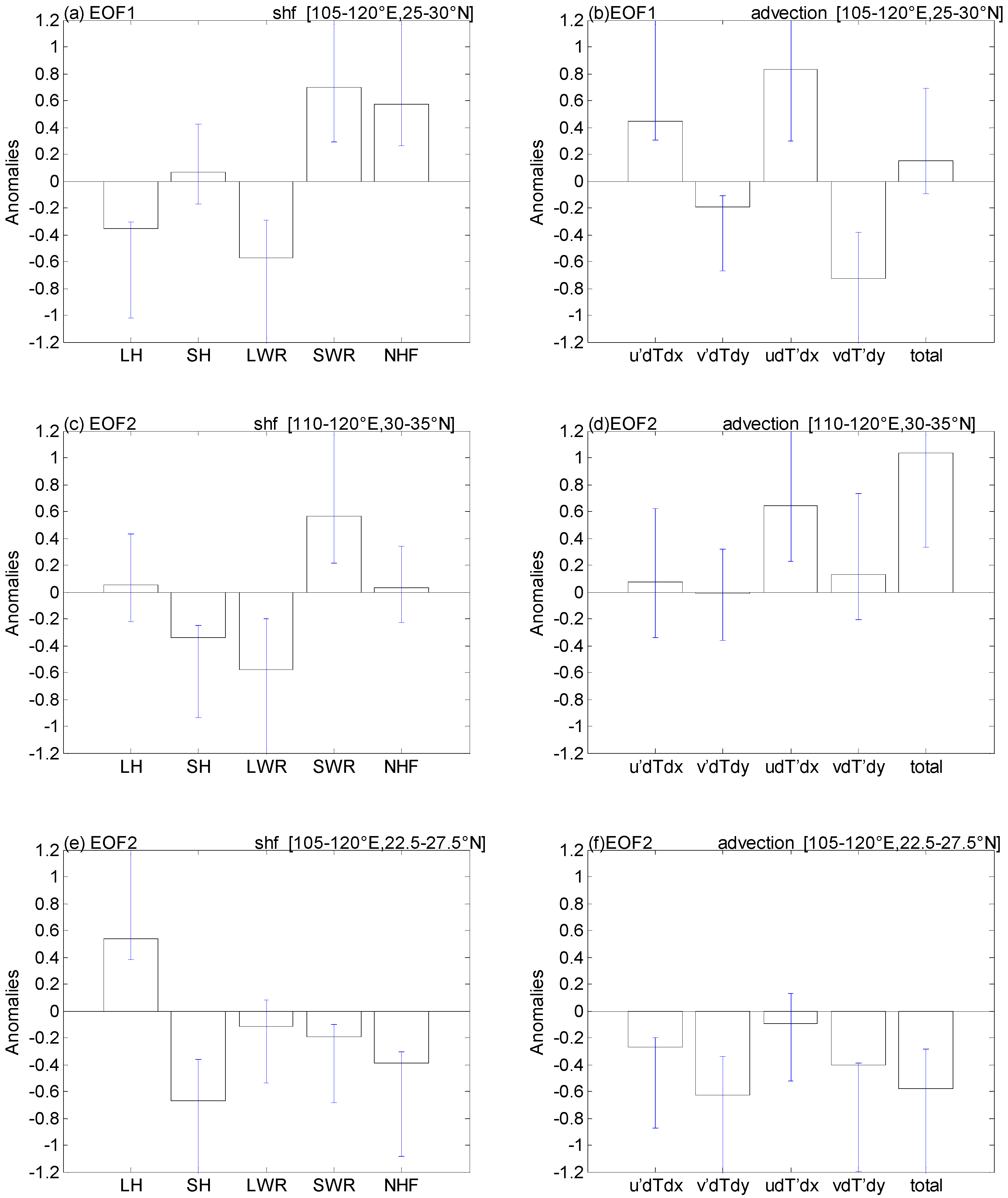
4.3. Comparison of Areal Mean Anomalies

To further quantitatively describe the contributions of surface heat flux and advection to SAT changes, we calculated their mean anomalies in selected regions with significant SAT anomalies (Figure 1a,b).

For EOF1, we selected central SC (105°–120° E, 25°–30° N), where a large increase in net SWR and a small increase in SH are partly cancelled by decreases in net LWR and LH, but their sum (NHF) results in a large net increase (Figure 6a). Advection shows an insignificant enhancement, as increases in $-u^{\prime }\frac{\partial \overline{T}}{\partial x}$ and $-\overline{u}\frac{\partial T^{\prime }}{\partial x}$ are cancelled by large decreases in $-\overline{v}\frac{\partial T^{\prime }}{\partial y}$ and $-v^{\prime }\frac{\partial \overline{T}}{\partial y}$ (Figure 6b). Overall, an increase in NHF plays an important role in the SAT anomalies of the EOF1 mode, and SWR is the main contributor to SAT increase.

For EOF2, we selected northern SC (110°–120° E, 30°–35° N) and southern SC (105°–120° E, 22.5°–27.5° N) for analysis. In northern SC, decreases in SH and LWR offset the increase in SWR and LH, leading to an insignificant increase in NHF (Figure 6c). For advection, $-u^{\prime }\frac{\partial \overline{T}}{\partial x}$, $-\overline{u}\frac{\partial T^{\prime }}{\partial x}$, and $-\overline{v}\frac{\partial T^{\prime }}{\partial y}$ all increase, leading to a positive contribution to warm SAT anomalies (Figure 6d). In southern SC, the main contributors to the decrease in NHF are SH, LWR, and SWR (Figure 6e). For advection, each component of advection decreases, leading to a large decrease in net advection. This favors cool SAT anomalies in southern SC (Figure 6f). In summary, advection plays an important role in the SC AMJ SAT anomalies of the EOF2 mode. In addition, NHF causes SAT changes in southern SC.

5. Conclusions and Discussion

This study investigates the spatiotemporal characteristics of the dominant modes of spring-to-summer SAT interannual variations and related physical processes over SC during 1948–2017. Results suggest that SAT anomalies corresponding to EOF1 have a homogeneous structure throughout SC, whereas the EOF2 mode shows a dipole pattern about the Yangtze River (~30° N) in SC.

Regression analysis indicates that surface heat fluxes, mainly influenced by cloud-SWR effects, play an important role in the SAT anomalies of EOF1 over SC. For EOF1, increases in SH over areas near 30° N make a positive contribution to warm SAT anomalies. And fewer clouds may lead to an increase in SWR anomalies, giving rise to warm SAT anomalies. NHF makes a significant positive contrition to warm SAT anomalies over SC, which reveals the important contribution of NHF to SAT. For EOF2, decreases in SH and increases in LH cancel each other out, leading to an insignificant net contribution to SAT. The distributions of SWR, LWR, and TCC anomalies are similar to the north–south dipole pattern of the SAT anomalies. This suggests that cloud-radiation processes control the warm (cool) SAT anomalies of the EOF2 mode over SC.

Further analysis shows that temperature advection plays an important role in the dipole-pattern SAT anomalies of EOF2 over SC. For EOF1, significant warm advection is observed east of 110° E. For EOF2, significant warm advection contributes to warm SAT anomalies north of 30° N. Significant cool advection is observed south of 30° N, contributing to cool SAT anomalies. Cool advection is caused mainly by the climatological temperature from northerly wind anomalies over land surfaces in high-latitude regions. Warm (cool) advection is caused mainly by the climatological temperature from southerly (northerly) wind anomalies or anomalous temperatures from climatological southerly (northerly) winds.

The study of climate change during the spring-to-summer transition deserves further investigation. Seasonal mean (averaged April–June) is a commonly applied method in previous studies. It presents a persistent state for climate anomaly from spring to summer and may contribute to summer climate anomalies [21]. As such, studying the AMJ-mean SAT anomalies over SC and its factor can improve the climate prediction not only in the transition season but also in summer. In addition, to emphasize the characteristics of spring-to-summer, Wu [21,22] used anomaly change from April to June (the anomaly in June minus the anomaly in April, denoted as the JmA anomaly) to show the advanced or a delayed transition. It is different from AMJ mean on the factors and processes of climate changes. For SAT anomalies over SC during spring-to-summer, this research method is very valuable for reference and can help for the further research.

This work focuses on SC SAT variations and their contributing factors during the spring-to-summer transition from 1948 to 2017. Several questions worthy of further investigation remain. Because SAT is correlated with cloud presence, what is its relationship with large-scale circulation? What caused the PC1 phase conversion in 1993 in the time series of SAT anomalies? What are the spatiotemporal characteristics of the dominant modes of SAT variations on the interdecadal scale? These questions should be the focus of future work.

References

1. Changnon, S.A.; Kunkel, K.E.; Reinke, B.C. Impacts and responses to the 1995 heat wave: A call to action. Bull. Am. Meteorol. Soc. 1996, 77, 1497–1506. [Google Scholar] [CrossRef]
2. Tan, J.; Zheng, Y.; Song, G.; Kalkstein, L.S.; Kalkstein, A.J.; Tang, X. Heat wave impacts on mortality in Shanghai, 1998 and 2003. Int. J. Biometeorol. 2007, 51, 193–200. [Google Scholar] [CrossRef]
3. Ding, T.; Ke, Z. Characteristics and changes of regional wet and dry heat wave events in China during 1960–2013. Theor. Appl. Climatol. 2015, 122, 651–665. [Google Scholar] [CrossRef]
4. Sun, Y.; Wang, S.; Yang, Y. Studies on cool summer and crop yield in Northeast China. Acta Meteorol. Sin. 1983, 41, 313–321. [Google Scholar]
5. Yao, P. The climate features of summer low temperature cold damage in Northeast China during recent 40 years. J. Catastrophol. 1995, 10, 51–56. [Google Scholar]
6. Wang, H. The weakening of the Asian monsoon circulation after the end of 1970’s. Adv. Atmos. Sci. 2001, 18, 376–386. [Google Scholar]
7. Song, F.; Zhou, T.; Qian, Y. Responses of East Asian summer monsoon to natural and anthropogenic forcings in the 17 latest CMIP5 models. Geophys. Res. Lett. 2014, 41, 596–603. [Google Scholar] [CrossRef] [Green Version]
8. Hu, X.; Liu, X. Decadal Relationship between Winter Air Temperature in Northeast China and Arctic Oscillations. J. Nanjing Inst. Meteorol. 2005, 5, 640–648. [Google Scholar]
9. Zhuang, Y.; Zhang, J.; Wang, L. Variability of cold season surface air temperature over northeastern China and its linkage with large-scale atmospheric circulations. Theor. Appl. Climatol. 2018, 132, 1261–1273. [Google Scholar] [CrossRef]
10. Kang, L.; Chen, W.; Wei, K. The interdecadal variation of winter temperature in China and its relation to the anomalies in atmospheric general circulation. Clim. Environ. Res. 2006, 11, 330–339. [Google Scholar]
11. Miyazaki, C.; Yasunari, T. Dominant interannual and decadal variability of winter surface air temperature over Asia and the surrounding oceans. J. Clim. 2008, 21, 1371–1386. [Google Scholar] [CrossRef]
12. Xu, X.; Li, F.; He, S.; Wang, H. Subseasonal Reversal of East Asian Surface Temperature Variability in Winter 2014/15. Adv. Atmos. Sci. 2018, 35, 737–752. [Google Scholar] [CrossRef]
13. Wang, B.; Yang, S.; Liu, S.; Sun, L.; Lian, Y.; Gao, Z. Changes in the relationship between Northeast China summer temperature and ENSO. J. Geophys. Res. Atmos. 2010, 115, D21. [Google Scholar]
14. Wang, B.; Yang, S.; Liu, S.; Sun, L.; Lian, Y.; Gao, Z. Northeast China summer temperature and North Atlantic SST. J. Geophys. Res. Atmos. 2011, 116, D16. [Google Scholar]
15. Wang, B.; Zhao, P.; Liu, G. Change in the contribution of spring snow cover and remote oceans to summer air temperature anomaly over Northeast China around 1990. J. Geophys. Res. Atmos. 2014, 119, 663–676. [Google Scholar] [Green Version]
16. Chen, W.; Hong, X.; Lu, R.; Jin, A.; Jin, S.; Nam, J.-C.; Shin, J.H.; Goo, T.Y.; Kim, B.-J. Variation in summer surface air temperature over Northeast Asia and its associated circulation anomalies. Adv. Atmos. Sci. 2016, 33, 1–9. [Google Scholar] [CrossRef]
17. Liang, P.; Lin, H.; Ding, Y. Dominant modes of subseasonal variability of East Asian summertime surface air temperature and their predictions. J. Clim. 2018, 31, 2729–2743. [Google Scholar] [CrossRef]
18. Wu, R.; Wang, B. Interannual variability of summer monsoon onset over the western North Pacific and the underlying processes. J. Clim. 2000, 13, 2483–2501. [Google Scholar] [CrossRef]
19. Wu, R.; Wang, B. Multi-stage onset of the summer monsoon over the western North Pacific. Clim. Dyn. 2001, 17, 277–289. [Google Scholar] [CrossRef]
20. He, Z.; Wu, R. Seasonality of interannual atmosphere–ocean interaction in the South China Sea. J. Oceanogr. 2013, 69, 699–712. [Google Scholar] [CrossRef]
21. Wu, R.; Hu, W. Air–Sea Relationship Associated with Precipitation Anomaly Changes and Mean Precipitation Anomaly over the South China Sea and the Arabian Sea during the Spring to Summer Transition. J. Clim. 2015, 28, 7161–7181. [Google Scholar] [CrossRef]
22. Wu, R.; He, Z. Two Distinctive Processes for Abnormal Spring to Summer Transition over the South China Sea. J. Clim. 2017, 30, 9665–9678. [Google Scholar] [CrossRef]
23. He, J.; Zhu, Q.; Murakami, M. TBB data-revealed features of Asian-Australian monsoon seasonal transition and Asian summer monsoon establishment. J. Trop. Meteorol. 1996, 12, 34–42. [Google Scholar]
24. Zhang, Y.; Wu, G. Diagnostic Investigations on the Mechanism of the Onset of Asian Summer Monsoon and Abrupt Seasonal Transitons over the Northern Hemisphere Part: II The Role of Surface Sensible Heating over Ti Betan Plateau and Surrounding Regions. Acta Meteorol. Sin. 1999, 57, 56–73. [Google Scholar]
25. Yao, S.; Zhang, Y. Effects of Surface Heat Flux on Surface Air Temperature Variation Trend in East Asia Region from Spring to Summer. Plateau Meteorol. 2007, 26, 240–248. [Google Scholar]
26. Fan, Y.; Van den Dool, H. A global monthly land surface air temperature analysis for 1948–present. J. Geophys. Res. Atmos. 2008, 113, D1. [Google Scholar] [CrossRef]
27. Matei, D.; Pohlmann, H.; Jungclaus, J.; Müller, W.; Haak, H.; Marotzke, J. Two tales of initializing decadal climate prediction experiments with the ECHAM5/MPI-OM model. J. Clim. 2012, 25, 8502–8523. [Google Scholar] [CrossRef]
28. Garcia-Serrano, J.; Frankignoul, C. High predictability of the winter Euro–Atlantic climate from cryospheric variability. Nat. Geosci. 2014, 7, E1. [Google Scholar] [CrossRef]
29. Willmott, C.J.; Matsuura, K. Terrestrial Air Temperature and Precipitation: Monthly and Annual Time Series (1950–1996). 2001. Available online: http://climate.geog.udel.edu/~climate/html_pages/README.ghcn_ts2.html (accessed on 3 February 2019).
30. Kalnay, E.; Kanamitsu, M.; Kistler, R.; Collins, W.; Deaven, D.; Gandin, L.; Iredell, M.; Saha, S.; White, G.; Woollen, J.; et al. The NCEP/NCAR 40-Year Reanalysis Project. Bull. Am. Meteorol. Soc. 1996, 77, 437–472. [Google Scholar] [CrossRef]
31. Kobayashi, C.; Iwasaki, T. Brewer-Dobson circulation diagnosed from JRA-55. J. Geophys. Res. Atmos. 2016, 121, 1493–1510. [Google Scholar] [CrossRef]
32. North, G.R.; Bell, T.L.; Cahalan, R.F.; Moeng, F.J. Sampling Errors in the Estimation of Empirical Orthogonal Functions. Mon. Weather Rev. 1982, 110, 699–706. [Google Scholar] [CrossRef] [Green Version]
33. Zhang, X.H.; Yu, Y.Q.; Liu, H. Wintertime North Pacific surface heat flux anomaly and air-sea interaction in a coupled ocean-atmosphere model. Sci. Atmos. Sin. 1998, 22, 511–521. [Google Scholar]
34. Li, D.; Li, W.; Li, W.; Lanzhi, L.; Hailing, Z.; Guoliang, J. A diagnostic study of surface sensible heat flux anomaly over the Qinghai-Xizang Plateau. Clim. Environ. Res. 2003, 8, 71–83. [Google Scholar]
35. Zhu, X.-S.; Zhang, Y.-C. Parameterization of subgrid topographic slope and orientation in numerical model and its effect on regional climate simulation. Plateau Meteorol. 2005, 24, 136–142. [Google Scholar]
36. Li, Y.; Li, J.; Kucharski, F.; Feng, J.; Zhao, S.; Zheng, J. Two leading modes of the interannual variability in South American surface air temperature during austral winter. Clim. Dyn. 2018, 51, 2141–2156. [Google Scholar] [CrossRef]
Figure 1. Spatiotemporal distribution of April, May, and Jume (AMJ) surface air temperature (SAT) interannual anomalies (K) over South China (SC) (20°–35° N, 105°–125° E) during 1948–2017. (a) EOF1 and (b) EOF2 of SAT anomalies, obtained by regression on normalized principle components (PCs). (c) PC1 and (d) PC2, representing the normalized PC time series corresponding to EOF1 and EOF2, respectively. Stippling denotes significant anomalies (95% confidence level, Student’s t-test). Significant SAT-anomaly regions are indicated by the black boxes in (a) and (b) and are used for calculating averaged anomalies for these regions.
Atmosphere 10 00065 g001
Figure 2. Anomalies in AMJ (a) net heat flux (NHF), (b) sensible heat flux (SH), (c) latent heat flux (LH), (d) net shortwave radiation (SWR), and (e) net longwave radiation (LWR) obtained by regression on the normalized PC1 of AMJ SAT during 1948–2017(W·m−2). Positive surface heat flux anomalies are downward, representing heat gained by the surface, and negative downward flux anomalies represent heat lost by the surface. Stippling denotes significant anomalies (95% confidence level, Student’s t-test).
Atmosphere 10 00065 g002
Figure 3. As in Figure 2, but for anomalies regressed on the normalized PC2 of AMJ SAT during 1948–2017.
Atmosphere 10 00065 g003
Figure 4. Anomalies in AMJ TCC obtained by regression on the normalized (a) PC1 and (b) PC2 of AMJ SAT during 1948–2017 (%). Stippling denotes significant anomalies (95% confidence level, Student’s t-test).
Atmosphere 10 00065 g004
Figure 5. Anomalies in AMJ (b) advection by wind anomalies, (c) advection by climatological wind, and (a) the sum of (b) and (c) at 1000 hPa by regression on the normalized PC1 of AMJ SAT during 1948–2017 (10−6 K·s−1). (d)–(f) As in (a)–(c), but for anomalies regressed on the normalized PC2 (10−6 K·s−1). Arrows in (b) and (e) (m·s−1) refer to wind anomalies regressed on PC1 and PC2, with magnitude greater than 0.8 m·s−1. Arrows in (c) and (f) refer to the AMJ climatological wind regressed on PC1 and PC2, with magnitude greater than 0.6 m·s−1. Stippling denotes significant anomalies (95% confidence level, Student’s t-test).
Atmosphere 10 00065 g005
Figure 6. Anomalies in surface heat flux (including LH, SH, net LWR, net SWR, and NHF averaged) over (a) central SC (105°–120° E, 25°–30° N; Figure 1a) regressed on the normalized PC1, (c) northern SC (110°–120° E, 30°–35° N; Figure 1b) regressed on the normalized PC2, and (e) southern SC (105°–120° E, 22.5°–27.5° N; Figure 1b) regressed on the normalized PC2 of AMJ SAT during 1948–2017 (W·m−2). (b), (d), (f) As in (a), (c), (e) but for anomalies in advection (including u T ¯ x , v T ¯ y , u ¯ T x , v ¯ T y and their sum; 10−6 K·s−1). All values are reliable with a high level of confidence.
Atmosphere 10 00065 g006