1. Introduction
DNA-binding proteins play a vital role in many biological processes, for instance DNA replication, transactional regulation, DNA repair and DNA modification [
1]. It is highly desired to develop computational methods to identify these proteins because of the time consumption and high cost in using experimental techniques such as filter binding assays [
2] and X-ray crystallography [
3]. So far, many computational methods based on machine learning have been proposed to identify these proteins [
4]. Building a meaningful feature set and choosing an appropriate classification algorithm are the two most trivial tasks [
5].
Building a feature set usually involves two steps: feature extraction and feature transformation. However, there is no clear boundary in using these two terms. To eliminate confusion, we use the first term to denote both cases in this paper. The information extracted includes sequence-based features [
6,
7] and structure-based features [
8].
The sequence-based feature extraction methods make full use of sequence composition, physiochemical properties and evolutionary information. Liu et al. proposed a protein feature vector representation composed of three kinds of features including overall amino acid composition, Pseudo Amino Acid Composition (PseAAC) and physiochemical distance transformation [
9]. They further improved the model by incorporating the evolutionary information by using profile-based protein representation [
10]. Xu et al. transformed the Position-Specific Scoring Matrix (PSSM) profiles into uniform numeric vectors for presenting protein sequences by the distance transformation scheme [
11]. In [
12], the protein sequences represented in the form of amino acids or the physical-chemical properties of amino acids were converted into a series of fixed-length vectors by K-mer composition and the auto-cross covariance transformation. Zhang et al. built feature sets by extracting the evolutionary information from the Position-Specific Frequency Matrix (PSFM), including Residue Probing Transformation (RPT), Evolutionary Difference Transformation (EDT), Distance-Bigram Transformation (DBT) and Trigram Transformation (TT) [
13].
As for the structure-based features, they often outperform the sequence-based features because they are more discriminating in identifying DNA-binding proteins. However, the structural information of the protein sequence is not always available because the structure of some protein sequences is unknown [
14]. Structural information such as motifs and secondary structures are important for identifying DNA-binding proteins. Chowdhury et al. used sequence evolutionary and structural information embedded in the protein sequences as features, in which the structural information was extracted using the SPIDER 2 software [
15,
16,
17].
There are many classification algorithms applied to identify DNA-binding proteins, such as support vector machine [
13,
17,
18,
19,
20], Gaussian naive Bayes [
21] and Random Forests(RF) [
22,
23]. Many existing methods employ only a single classification algorithm. The single classifier has its own inherent defects [
24]. For instance, SVM has high computational complexity, and its performance relies heavily on its parameters. Logistic regression requires huge samples to achieve stable performance [
25]. Comparing to the single classifier, ensemble learning tries to train multiple models using base classifiers, then combines them to make the final predictions [
26,
27]. There are many effective ensemble strategies such as boosting, bagging, stacking and majority voting. Xu et al. [
28] employed the unbalanced-AdaBoost to predict DNA-binding proteins using features of residue/dipeptide compositions and distributions. Song et al. [
29] adopted 16 base classifier algorithms and applied the weighted voting to identifying DNA-binding proteins using 188Dfeatures. Liu et al. [
27] used the SVM as the base classifier and applied weighted voting to make the final prediction, in which the weights were gained by the grid search.
Having inherent parallelization and a flexible combination and mathematical evaluation of base models, stacking is often used in computationally intensive scenarios with the particular intention to investigate the contributions of base models. Zou et al. applied a stacking-based method for identifying DNA-binding proteins using four types of feature vectors covering global, non-local and local protein sequence information, in which SVM was adopted as both the base and combination model [
30].
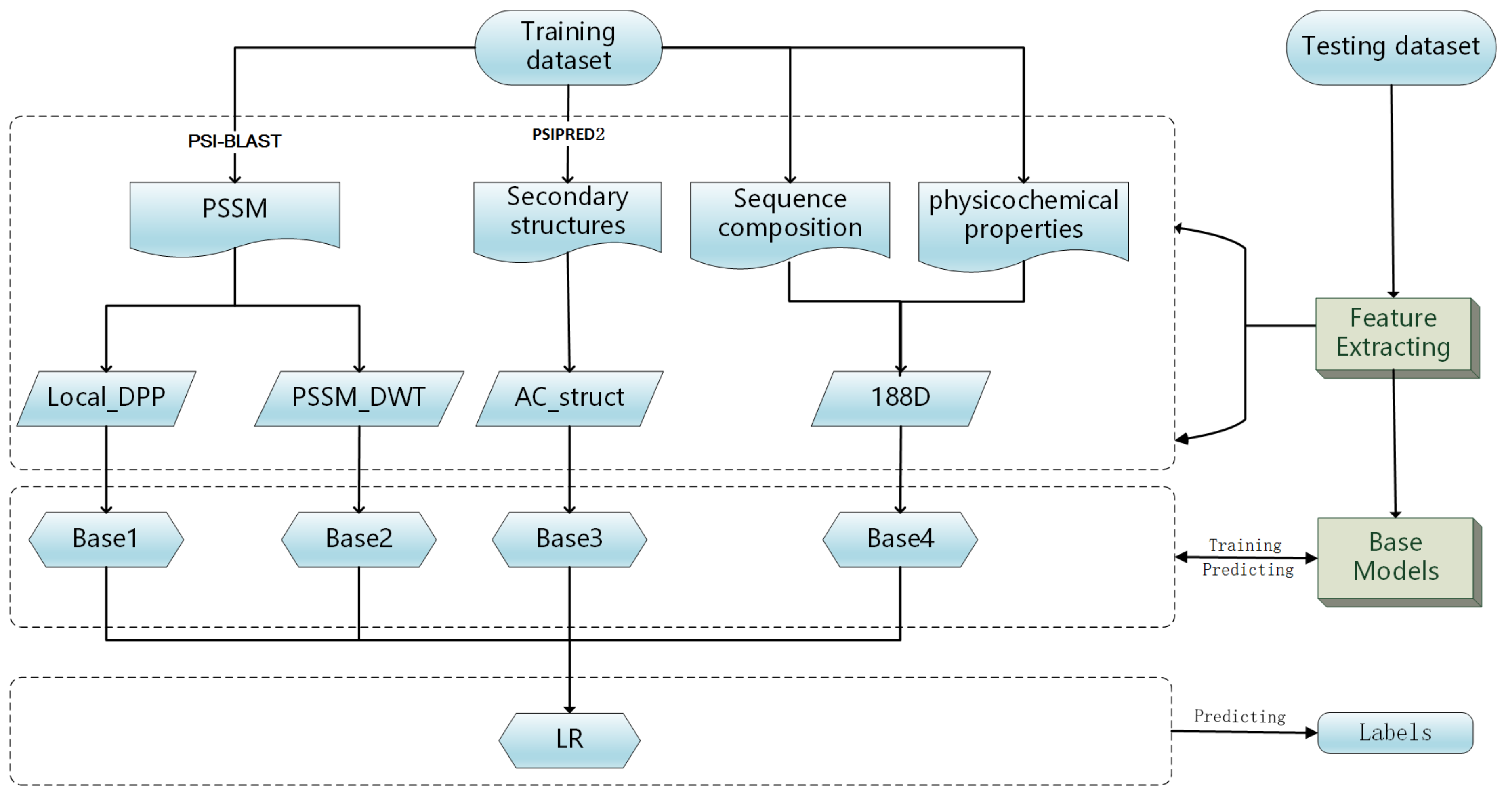
In this work, we propose a model stacking framework by orchestrating multi-view features and classifiers (MSFBinder) to investigate how to integrate and evaluate loosely-coupled models for predicting DNA-binding proteins. The framework integrates multi-view features including Local_DPP [
22], 188D [
31], PSSM_DWT [
32] and AC_struct [
33] for secondary structures, which are extracted based on evolutionary information, sequence composition, physiochemical properties and predicted structural information, respectively. These features are fed into various loosely-coupled classifiers such as SVM and random forest. Then, a Logistic Regression (LR) is applied to evaluate the contributions of these individual classifiers and to make the final prediction. Within the framework, we first train SVM classifiers on the four feature spaces independently to show their prediction effectiveness. Then, we build three predictors including both homogeneous (SVM) and heterogeneous (SVM, Random Forest (RF) and Naive Bayes (NB)) base models. After plotting and T-test analysis of LR coefficients on both the training and independent test datasets, we find that RF prefers the features of PSSM_DWT, SVM likes Local_DPP features more and both of these two kinds of features play significant roles in the prediction of DNA-binding proteins. It is noteworthy that the NB classifier is more stable against all the features, although its coefficients are not too high. Meanwhile, all three predictors outperform the single classifiers, and there is no big performance difference between homogeneous and heterogeneous base models. Finally, we show that the overall performance of MSFBinder outperforms the state-of-the-art of existing methods on the independent testing dataset.
3. Results and Discussions
3.1. Performance Comparisons of Different Feature Representations Only Using SVM as the Training Model
In order to evaluate the prediction capability of the different feature extraction methods, the five-fold cross-validation was applied using SVM as the training model. As shown in
Table 4, most of the feature spaces achieved acceptable performance. Local_DPP beat all the other three with an accuracy of 78.32%, an MCC of 0.5681 and an SP of 75.63%. The results suggest that sequence order and the local evolutionary information contribute significantly to the prediction of DNA-binding proteins. The performance of AC_struct was inferior to the others. This might have been caused by the false predictions of the secondary structures by the PSIPRED 2 program.
3.2. Performance Comparisons Using Different Base Classifiers
In this section, we build three types of predictors: MSFBinder (SVM), MSFBinder (SVM, RF) and MSFBinder (SVM, RF, NB) in the MSFBinder framework. They were performed on four types of feature spaces using SVM, SVM + RF and SVM + RF + NB as the base classifiers and obtained 4, 8 and 12 models, respectively. Then these models are fed into the LR to make the final predictions. For each predictor, we compared their performances to two types of parameter setups of Local_DPP. The leave-one-out cross-validation was applied to evaluate the performances. The results on PDB1075 and PDB186 are shown in
Table 5 and
Table 6.
Table 5 shows that the second predictor with
and
achieved the best performance with
,
,
and
. The first predictor with
and
performed the worst with
,
,
and
. The gaps of ACC, MCC, SN and SP between the best and worst ones were 1.49%, 0.0299, 1.9% and 1.09%, respectively. For the test dataset shown in
Table 6, the first predictor with
and
achieved the best performance. The second predictor with
and
reached the worst case. The best one beat the worst one in terms of values of ACC, MCC, SN and SP by 2.69%, 0.0389, −3.22 and 8.6%, respectively. Although the first predictor performed slight worse on the training dataset, it worked best on the testing dataset. This suggests that the first predictor had good generalization. All three predictors outperformed the one only using SVM.
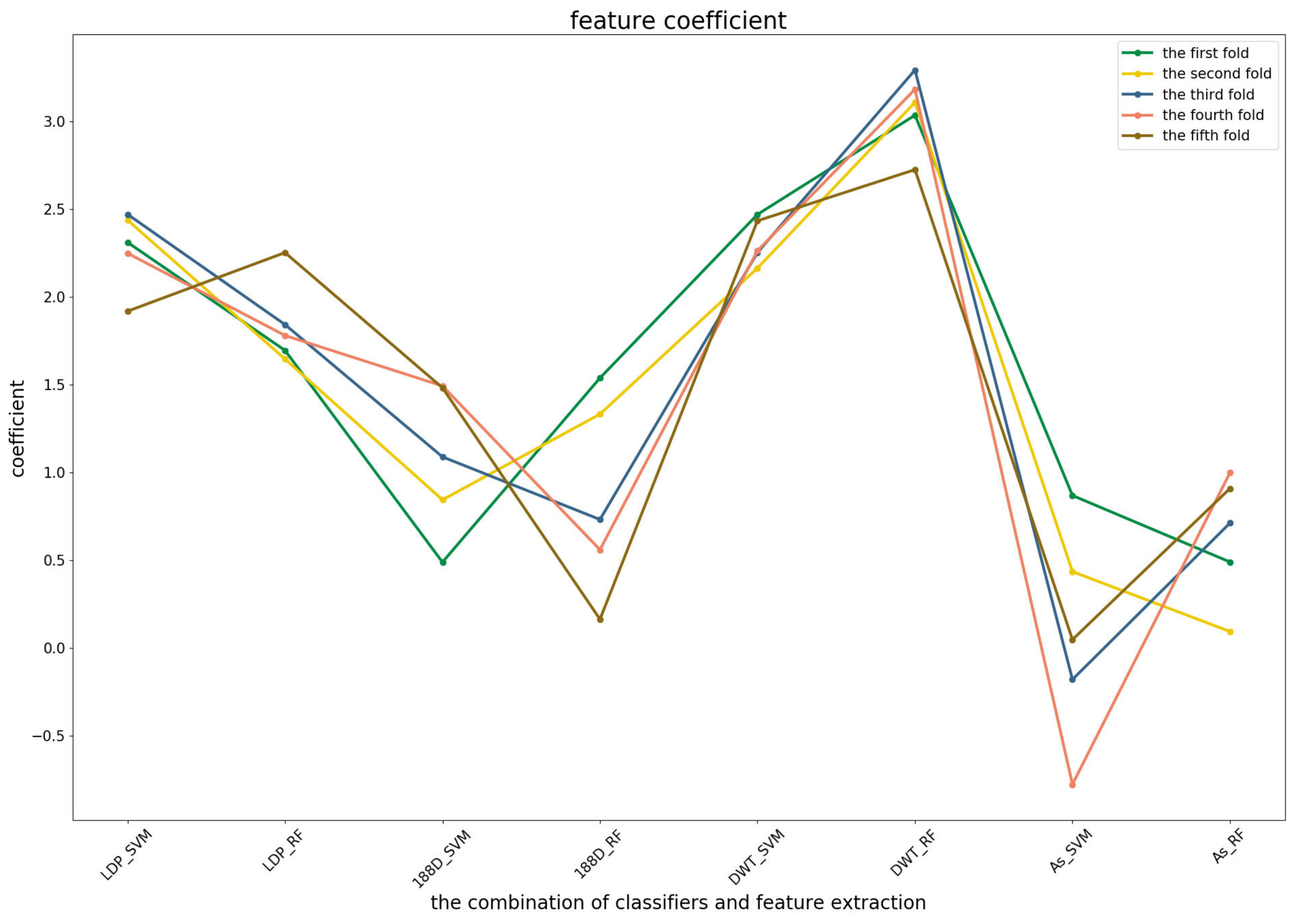
3.3. Significance Analysis of Different Base Models for Three Predictors
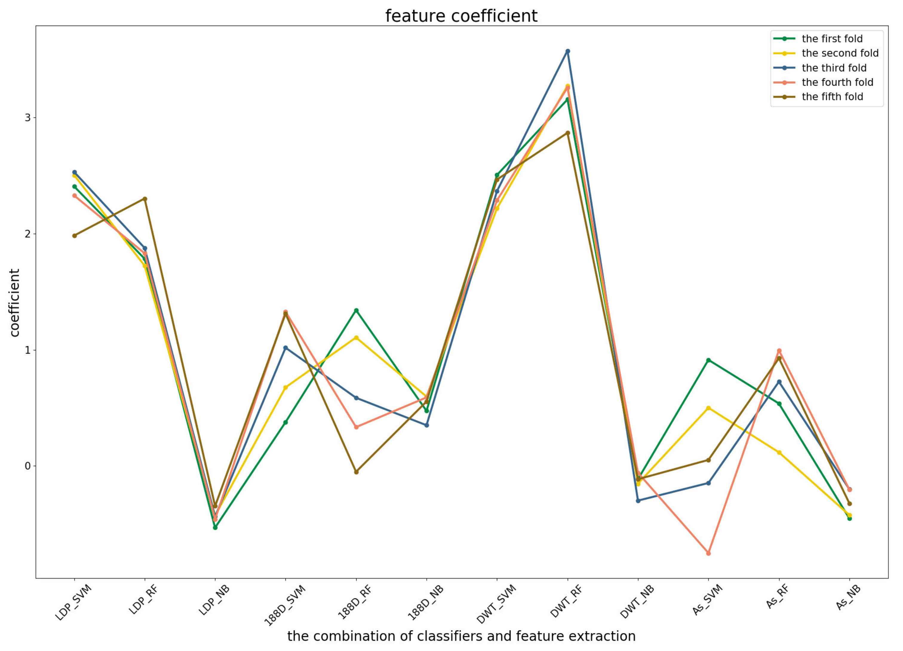
To further demonstrate the contributions of different base classifiers combined with corresponding feature representations for the final prediction, the LR coefficients of the base models for five-fold cross-validations are drawn in
Figure 3,
Figure 4 and
Figure 5, in which all the parameters of Local_DPP are set the same, as
and
.
In the first predictor (
Figure 3), the PSSM_DWT features contributed the greatest, then the Local_DPP features. Both features were more stable among all of the five-fold cross-validations. The other two features were heavily dependent on the datasets.
Figure 4 shows that the RF model preferred the features of PSSM_DWT, and their combination made the biggest contribution across all of the five-fold cross-validations. SVM combined with the Local_DPP features ranked second. Both two types of features worked well on the SVM and RF classifiers. The 188D features were not sensitive to the datasets for SVM and RF, while the contribution of AC_struct features was smaller than the others for all folds.
For the third predictor (
Figure 5), Local_DPP and PSSM_DWT features played similar roles as the second one for SVM and RF. Both of them had significant effects on the predictions. The 1880D features were sensitive to the datasets for RF and SVM, and a similar case applied to the AC_struct and SVM models. It should be noted that NB classifiers were more stable across all of the features, but have a lower contribution.
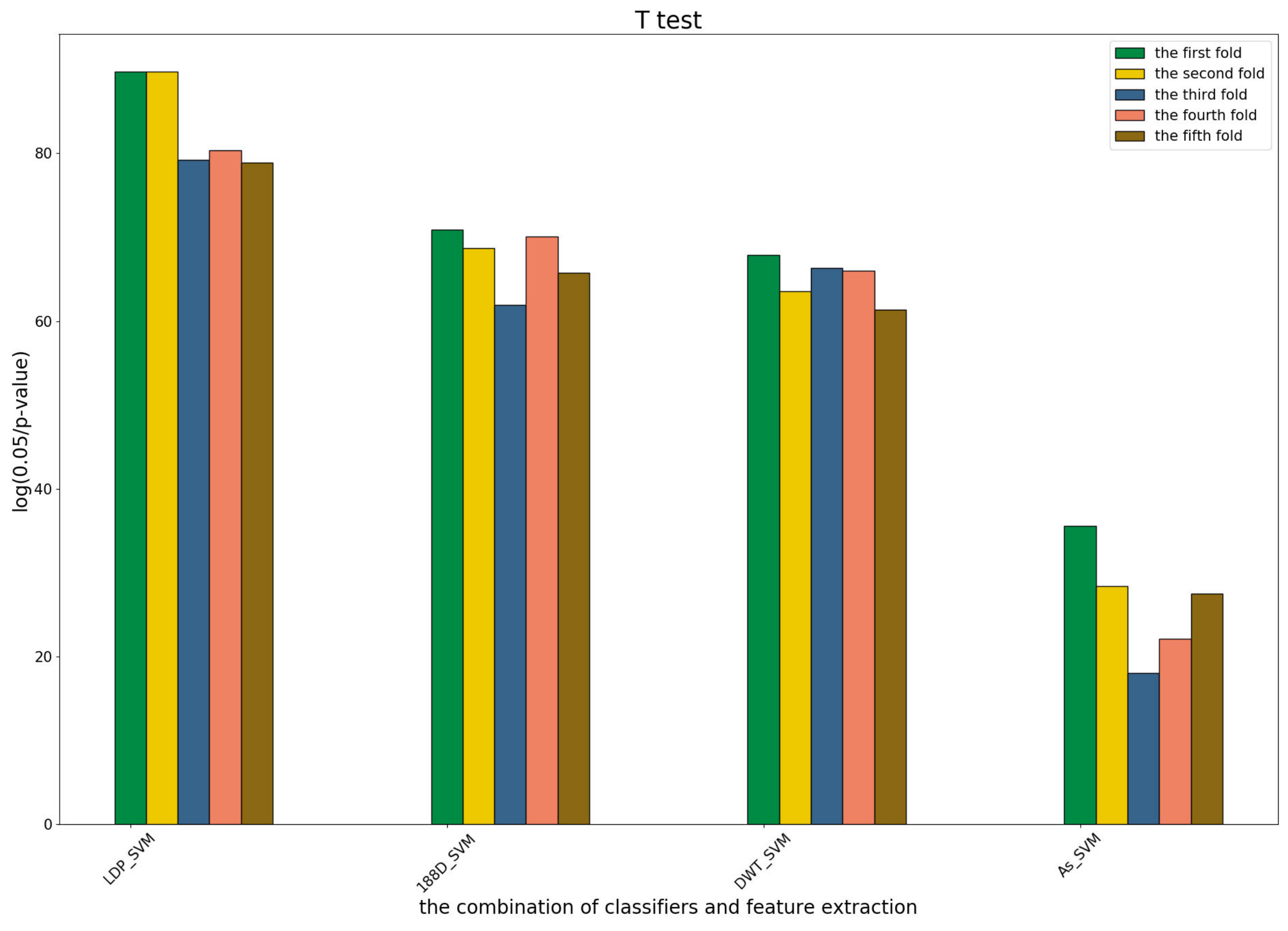
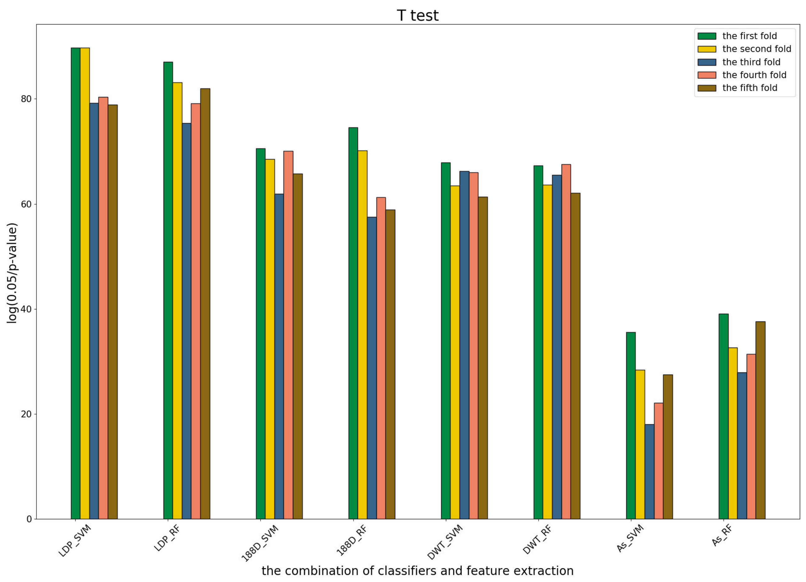
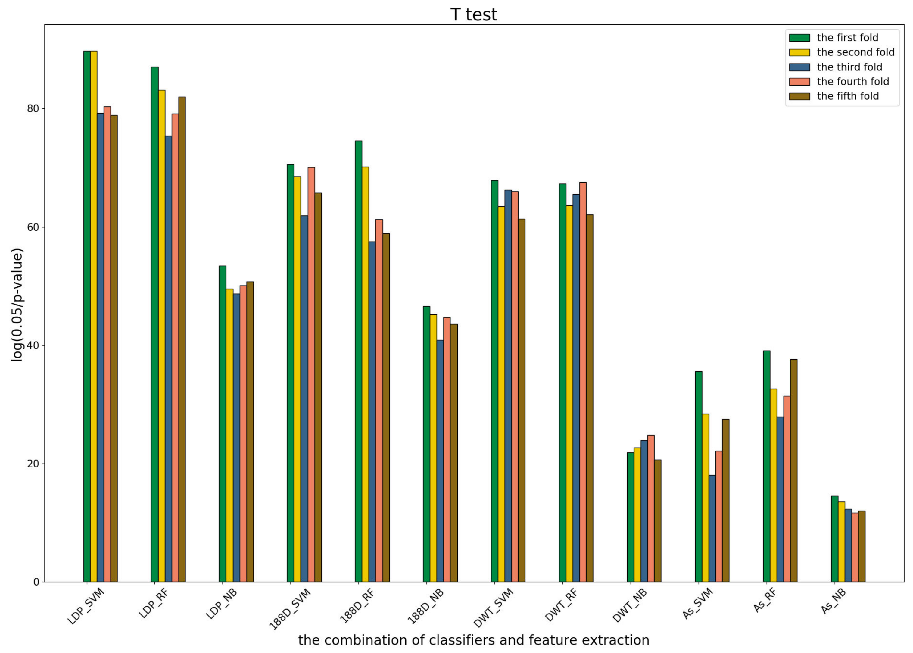
3.4. T-Test Analysis of Different Base Models for Three Predictors and Performance Measures
To further show the statistical significance of base models for the three predictors, we performed T-test analysis on the LR base models of each predictor for the five-fold cross-validations. The results are shown in
Figure 6,
Figure 7 and
Figure 8.
These results demonstrate that there was no big difference in the p-values for all the base models across all folds, except for the ones involved in the AC_struct features. SVM performed the best with all feature spaces.
3.5. Performance Comparisons with Single Classifiers
To verify the effectiveness of the presented method, we compared the performances to the ones only using the single classifiers by leave-one-out cross-validation. Three classifiers, SVM, RF and LR, were used. The results are shown in
Table 7. MSFBinder with
achieved better performance than any of the others, and MSFBinder with
performed slight worse than the first one. Among these single classifiers, the SVM model with
works the best with
,
,
and
. Though the SN value of MSFBinder was lower than the SVM model, its values of AC, MCC and the SP were higher than those of the other single classifiers.
3.6. Performance Comparisons with Majority Voting-Based Methods
The majority voting strategy is another popular method of model ensembling. It assigns the final class label of each sample using the one predicted by the (weighted) majority of base classifiers. We ran SVM, RF and LR on the four feature spaces, respectively, then the simple majority voting was applied to make the final predictions; see
Table 8 for the results. The ACC, MCC and SN values of MSFBinder were 1.93%, 3.83% and 1.73% higher than the best ones of majority voting-based methods, respectively. The MSFBinders with two types of parameters were both better than the majority voting methods. Compared to
Table 4, both kinds of model ensembling performed better than the models only using single classifiers.
3.7. Stability Comparisons with the Single Classifiers and Majority Voting Methods
The stability of a learning algorithm refers to the changes in the output of the system when we change the training dataset. A learning algorithm is said to be stable if the learned model does not change much when the training dataset is modified. There are several ways o modify the training set, such as choosing different subsets, using different feature sets and putting noise into the training set. Mathematically speaking, there are many ways of determining the stability of a learning algorithm. Some of the common methods include hypothesis stability, error stability and leave-one-out cross-validation stability.
Here, we tested the stability using different subsets by 5 × 5-fold cross-validation methods. By running the five-fold cross-validation five times on the training set using the four feature sets, the means and standard deviations of four evaluation metrics were calculated; see
Table 9.
The results show that MSFBinder achieved the best mean performance with , , and . It beat RF in terms of the values ACC, MCC, SN and SP by 2.34%, 0.0474, 3.37% and 1.59%, respectively. While RF beat the minimal standard deviations for all the measures, this suggests that RF was the most stable of them. The standard deviations for the above four measures in MSFBinder ranked 5, 5, 2 and 4 among seven methods, respectively.
3.8. Comparisons to Existing Methods
We compared the performances to other existing methods including IDNA-Protdis [
18], IDNA-Prot [
19], DNA-Prot [
54], DNAbinder [
20], Kmer1 + ACC [
12], Local-DPP [
22], PSSM_DT [
9], PSSM-DBT [
13], iDNAPro-PseAAC [
10] and iDNAProt-ES [
17]. The results are shown in
Table 10 for the training set and
Table 11 for the testing set.
On the training set, iDNAProt-ES ranked first for all the evaluation metrics, and MSFBinder ranked second except for the SP metrics. The best performance of iDNAProt-ES might lie in its feature set incorporating various transformations for both the sequence evolutionary information and predicted secondary structure information, while our method only used the auto-covariance features for predicted secondary structure information.
On the testing set, MSFBinder (n = 2, = 2) ranked the first in terms of ACC (81.72%), and its MCC (0.6417) and SN (93.55%) values were almost the same as the best ones (0.647 and 94.62%) of the others.
It is noteworthy that the values of its ACC, SN and SP were 6.65%, 6.57% and 6.73% higher than ours on the training dataset, while the values of ACC, MCC and SN in our method were 1.08%, 0.0287 and 7.94% higher than iDNAProt-ES. Thus, MSFBinder has better generalization ability than existing methods.


