Evaluation of FAO AquaCrop Model for Simulating Rainfed Maize Growth and Yields in Uganda


Department of Agricultural and Biosystems Engineering, Makerere University, Kampala, P.O. Box 7062, Uganda
*
Author to whom correspondence should be addressed.
Agronomy 2018, 8(11), 238; https://doi.org/10.3390/agronomy8110238
Submission received: 26 July 2018
/
Revised: 18 September 2018
/
Accepted: 28 September 2018
/
Published: 25 October 2018
(This article belongs to the Special Issue Agricultural Water Management)
Abstract
:Uganda’s agriculture is mainly rainfed. While farmers make efforts to increase food output to respond to the demands of a fast growing population, they are vulnerable to losses attributed to fluctuating weather patterns due to the global climate change. Therefore, it is necessary to explore ways of improving production in rainfed agricultural systems to save farmers labour and input costs in situations where the grain harvest would be zero due to crop failure. In this study, the Food and Agriculture Organization (FAO) AquaCrop model was evaluated for its predictability potential of maize growth and yields. The study was conducted at Makerere University Agricultural Research Institute Kabanyolo (MUARIK) in Uganda for three seasons. Maize growth and yield data was collected during the following seasons: Season 1, September to December 2014; Season 2, March to July 2015; and Season 3, September to December 2015. The model was calibrated using season 1 canopy cover data. The relative errors of simulated canopy cover ranged from −0.3% to −13.58% for different stages of the crop growth. The deviation of the simulated final biomass from measured data for the three seasons ranged from −15.4% to 11.6%, while the deviation of the final yield ranged from −2.8 to 2.0. These results suggest that FAO AquaCrop can be used in the prediction of rainfed agricultural outputs, and hence, has greater potential to guide management practices towards increasing food production.
1. Introduction
Maize is an important cereal crop in Uganda, cultivated on over 23.4% of the land dedicated to food crops [1]. Currently, maize is a major staple food for low income earners in rural and urban areas, providing a varied diet to households and institutions (schools, prisons, factories, etc.) in the form of roasted green cobs, steamed green cobs, and maize flour prepared as posho (maize porridge). Maize is a source of income for smallholder famers, providing a living to over 3.8 million Ugandans and a source of government revenue through foreign exchange, contributing to over US $ 100 million in forex earnings [1].
Over the years, Uganda’s agriculture has mostly depended on rainfall which is distributed in a bimodal pattern, with short rains coming between March to June and the long rains from September to December. For the period 1940 to 2009, annual rainfall amounts ranged from 660 to 1600 mm [2]. Because of this rainfall distribution, many parts of Uganda—with the exception of the northern part of the country—produce maize during the two seasons. The Northern region, which is a relatively drier area, produces maize in only one season (October to January).
However, the required rainfall for agricultural production is increasingly becoming unreliable due to climate change affecting rainfall distribution [3,4], and subsequently affecting food production. Data indicates that maize output is only 2.663 × 10⁶ tons from 1.149 × 10⁶ ha [5]. This output can’t respond to the needs of the growing population, i.e., 3.2% per annum [6], and hence, threatens food security. Thus, Uganda is food insecure, with 6% of Ugandans surviving on one meal a day, 14% of children stunted, and 48% of Ugandans being food energy deficient [7].
With the increasing threat of food insecurity on the population, there is a need for efficient and effective food production systems if the demands of the high population are to be met. However, these production systems require more water use, yet agricultural water use faces competition from other sectors like municipal, industrial, and ecological [8] activities. Although smart irrigation water saving technologies (rain sensor, soil water sensor and evapotranspiration controller) [9,10,11] have been developed, Uganda’s agriculture is dominated by small and medium scale farmers with national average land holding sizes of 1.1 ha [12]. These farmers cannot afford the investment and maintenance costs of systems such as smart irrigation equipment. Therefore, this study sought to find an alternative method to accurately predicate the yields (biomass and grain harvest) of Uganda’s staple crop, maize, under rainfed agriculture. This was in an attempt to save farmers labour and input costs in situations where the grain harvest would be zero due to crop failure. Rockström and Barron [3] showed that it is possible to at least double rainfed staple food production by producing more ‘crop per drop’ of rainwater. Crop yield simulation models like APSIM [13], DSSAT [14], and FAO AquaCrop [15] have been widely used as decision support tools in the agricultural sector.
However, these models are often applicable only to the fields for which they are calibrated, and require a number of parameters for their application, hence limiting their application in developing countries like Uganda, where there are challenges of data collection due to inadequate equipment and funds to conduct research.
The FAO AquaCrop model, originating from the “yield response to water” [16], developed in 2009 into a normalized crop water productivity concept [17,18]. In comparison to other models, the AquaCrop is relatively easy to run, as it requires only a set of easy to acquire input parameters [18,19]. The AquaCrop model is a robust model capable of simulating crop performance in multiple scenarios.
The AquaCrop model has been tested on grain crops in different environments, for example maize in California, USA [19], maize in Zaragoza, Spain [20], barley in Ethiopia [21], and maize in Kenya [22]. However, no such study has been reported for Uganda. Therefore, the purpose of this study was to assess the capability of the AquaCrop model to simulate the growth and yields of maize in Uganda.
2. Materials and Methods
2.1. Description of the Study Area
The study was conducted at the Makerere University Agricultural Research Institute Kabanyolo (MUARIK), Wakiso district, Uganda (Latitude 0°28′00.38″ N, Longitude 32°36′46.01″ E and 1161 m above sea level). The weather station at MUARIK is located at the following coordinates: Latitude 0°27′49.99″ N, Longitude 32°36′28.68″ E.
MUARIK is characterized by a typical tropical climate with average maximum temperatures of 28.5 °C and minimum temperatures of 14 °C. The mean annual rainfall approximates 1200 mm in a bimodal distribution, with the short rains coming between March to June, and the long rains from September to December [23]. The soil type is clay-loamy.
Longe5, popularly known as “Nalongo”, a local cultivar commonly grown by farmers, was used in the experiment, and the local practices of farm management (ploughing, weeding, pest management, no fertilizer amendments) were followed. Longe5 was released by the National Agricultural Research Organization in 2000 in response to farmers’ concerns about the low productivity of maize crops in Uganda. Farmers have shown a preference for this variety because of its quality protein, easy access to seed, and good adaptability [24]. Plot area was 64 m2 in all the growing seasons, replicated three times in a randomized complete block design. Some of the relevant information required for the model is presented in the Table 1. The September to December 2014 season received high precipitation, averaging 5.12 mm/day, and fairly distributed throughout the whole season. In contrast, the March to July 2015 season had relatively low precipitation, averaging 2.82 mm/day, with low downfall at the start of the season and gradually decreasing rainfall towards the end. The September to December 2015 season had high rainfall, averaging 5.31 mm/day and fairly distributed throughout the entire season. The mean seasonal temperature was 20 °C. The mean annual air humidity was 78%, and the average wind speed at a height of 2 m was 3.2 m/s.
2.2. Model Input Data
Weather data (Rainfall, mm; Sunshine hours, h; Wind speed, m/s; Temperature, °C and Relative humidity, %), were obtained from the MUARIK weather station located 0.60 km southwest of the experimental field. The Mean annual atmospheric carbon dioxide concentration for recent years, measured at Mauna Loa Observatory in Hawaii, is provided in the AquaCrop and regularly updated [20]. The daily reference evapotranspiration (ETo) for each growing season was calculated based on the FAO Penman-Monteith method [25] using the ETo calculator [26].
Three Soil samples were collected from the study area for each of the four laboratory analyses. The soil properties laboratory analysis results are presented in Table 2. However, permanent wilting point moisture content (Ɵwp), field capacity moisture content (Ɵfc), and hydraulic conductivity at saturation (ksat) were the only properties recommended as model inputs as Heng et al. [20]. The saturated hydraulic conductivity was obtained by a constant head method; the soil moisture content at field capacity and wilting capacity were obtained by the pressure plate apparatus method [27]. Given the soil type and the plant patterns, the Curve Number (CN) for the field was 67 [28]. The Readily Evaporative water value used in the model was 5 mm.
The AquaCrop model uses three categories of crop parameters. Conservative parameters (Table 3) do not necessarily change with time, location, cultivar or management practices [19,20], and they are provided with the model. Management and cultivar specific parameters are also required by the model; these vary with cultivar and management. Some of these parameters are presented in Table 1.
2.3. Description of AquaCrop Model
The model was proposed by FAO in 2009, with the details outlined in Steduto et al. [18], and Raes et al. [15]. The model relates its components (the soil, the crop, and the atmosphere) through soil and water balance, the atmosphere (precipitation, temperature, evapotranspiration, and carbon dioxide concentration), and crop conditions (phenology, crop cover, root depth, biomass production, and harvestable yield) and field management (irrigation, fertility and field agronomic practices) components [17,18]. It computes the daily water balance and separates the evapotranspiration into evaporation and transpiration. Transpiration is associated with canopy cover which is proportional to the scope of soil cover, whereas evaporation is related to the area of soil not covered. As the crop matures, it responds to water changes through four stress coefficients (leaf expansion, stomata closure, canopy senescence, and change in harvest index). The AquaCrop uses a normalized crop water productivity (WP*) to calculate the daily aboveground biomass production [18,19], which is considered constant for a given climate and crop. The yield is obtained by multiplying the biomass with the harvest index (HI). The HI for maize was set between 48% and 52%.
2.4. Field Data Collection
The canopy cover values during the first season were obtained through aerial images of three randomly selected representative plants from each of the four experimental plots. The images were analyzed in Imagej software [29] to obtain the canopy cover.
Final biomass and grain yield was obtained following maturity using samples obtained from the experimental plot. The final aboveground biomass samples were collected by cutting the crop at the ground level; they were then oven dried for two days, and finally, weighed on a digital scale. The final yield samples were also harvested, dried to 12.5% moisture content in a drier, and weighed on the digital scale.
2.5. Model Evaluation Criterion
The model was calibrated using measured canopy cover accumulation values for the September to December 2014 growing season. The model was run after entering all the input data sets, and an iterative process was conducted by adjusting the model parameters until the best match between the simulated and measured data was obtained. The validation was done using the measured final biomass and grain yield against simulated values for all the three seasons.
The performance of the model was evaluated using statistical parameters which include Root Mean Square Error (RMSE) and Nash-Sutcliffe (E). E assesses the predictive power of the model [30] (Equation (1)), while RMSE (Equation (2)) indicates the error in model prediction; these statistical indices were used to compare the measured and simulated values.
where and are the simulated and observed data, is the mean value of , and N is the number of observations.
RMSE measures the overall deviation between observed and simulated values, thereby estimating the model uncertainty. It takes the same units of the variable being simulated, and therefore, the closer the value is to zero, the better the model simulation performance. However, E compared to RMSE evaluates the model performance over the entire simulation period. RMSE does not account for the large deviations occurring in some parts of the season, or the small deviations in other part of the season; E accounts for the different deviations, as they depart from () along the season and expresses an efficiency of the model performance, that is, the smaller the departure from (), the higher the performing efficiency of the model. E is unitless and may assume values ranging from −∞ to +1, with better model simulation efficiency when values are closer to +1.
3. Results and Discussion
3.1. Canopy Cover
The simulated and observed canopy cover values during the September–December, 2014 growing season are shown in Table 4. The AquaCrop could simulate the canopy cover (%) development for the entire growing season.
The relative errors of simulated canopy cover ranged from −0.3% to −13.58% for different stages of the crop growth. This implies that the model over simulated the canopy cover, and the simulation was varying at each stage of growth. However, the simulations at the start and the end of the growing period were not well simulated.
3.2. Final Biomass and Grain Yield
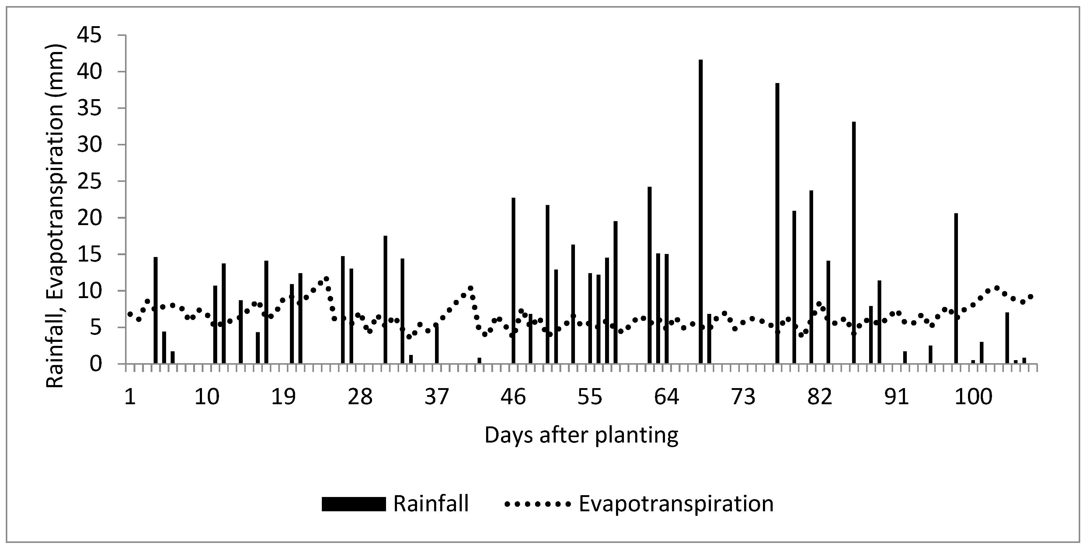
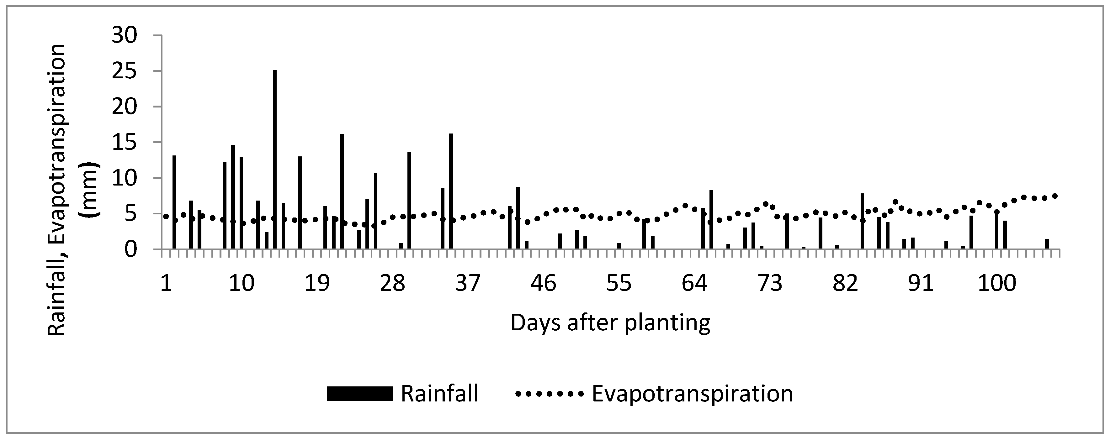
Figure 1 and Figure 2 show a comparison of the simulated and observed yield and biomass for all the growing seasons. Likewise, Figure 3, Figure 4 and Figure 5 show rainfall and evaporation regimes for the 3 growing seasons. The values of simulated and observed yield and biomass and percentage deviations are presented in Table 5. Results showed that the model simulated grain yield better than biomass. The values of RMSE and E for final yield and biomass simulations are also presented in Table 6.
The measured and simulated values for biomass and grain yield over the 3 seasons are given in Table 5. The relative errors of simulated biomass and yield ranged from −6.6% to 11.6% and 2.0% to 3.2%, respectively. The results show that the model simulated grain yield better than biomass.
From the results, it is observed that the model under simulated the final biomass compared to the final yield; hence, negative percentage deviations occurred for final biomass, and positive deviations occurred for final yield, except for the third season. However, these results, for both final yield and biomass, are comparable to the maize [19,31] and sweet sorghum simulation results [32].
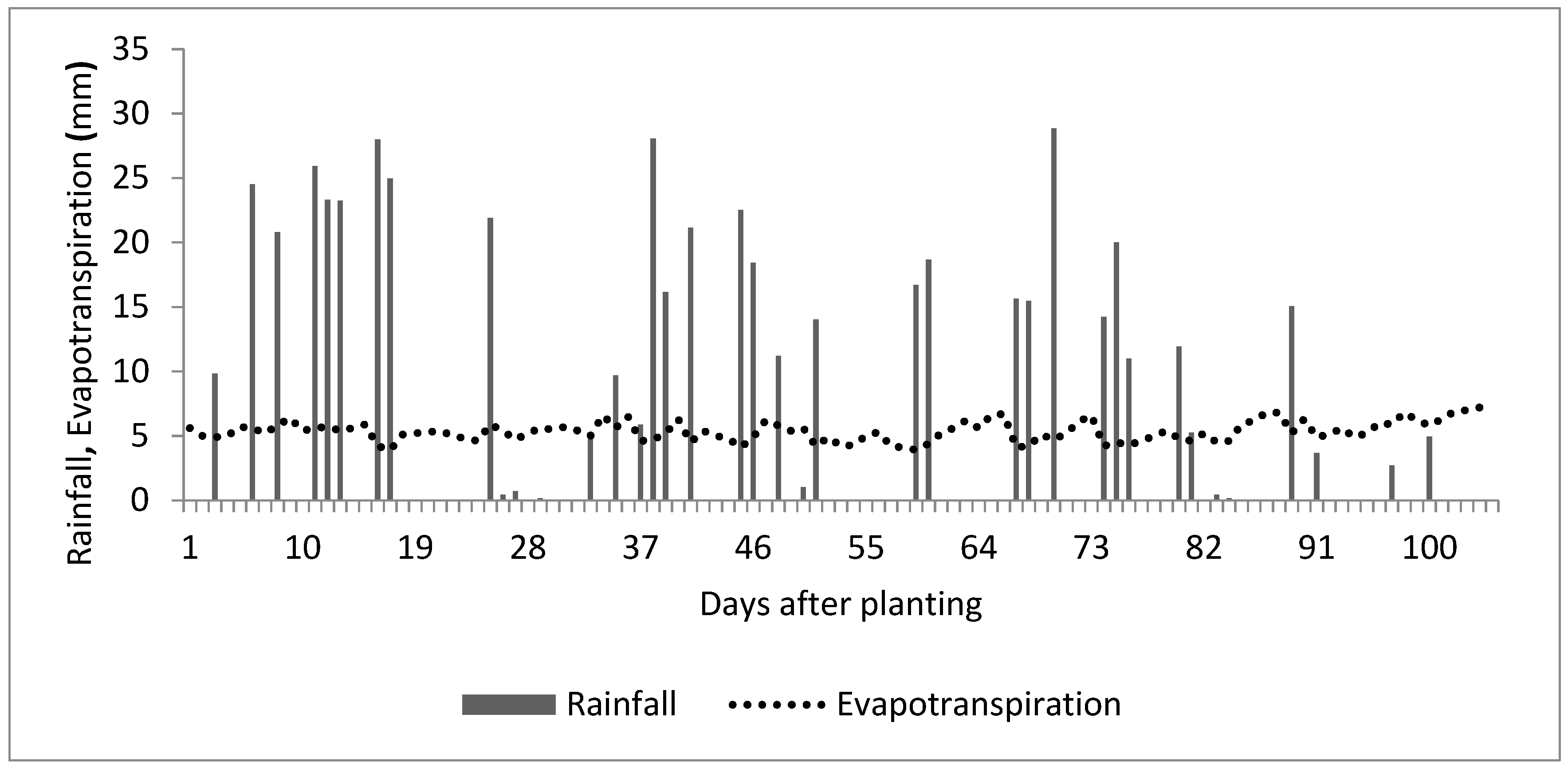
The maize production of the September to December 2015 growing season was greater compared to the proceeding seasons, as reflected in both final biomass and yield results. This was attributed to the high seasonal rains and seasonal evapotranspiration (Table 1). The rainfall and evapotranspiration were all high but evenly distributed throughout the entire season (Figure 3); hence, the crop never experienced any water stress.
Production in the September to December 2014 growing season was greater than that of March to July 2015. This is because the second season rains (September to December) in the study area are more intensive and evenly distributed than the first season rains (March to July). Therefore, during the March to July 2014 growing season, the crop experienced some water shortages during the critical growth stages, which subsequently contributed to low yields (Figure 5). Brouwer and Heibloem [33] observed that maize needs at least 500 mm of rainfall for good yields. The rainfall received during the March to July 2014 growing season was 320 mm.
The difference in the yields between the September to December growing seasons for 2014 and 2015 might have been a result of other factors, like pests, fertility, and management.
Statistical evaluation of the AquaCrop performance for the all growing seasons shows a better simulation for yield than biomass (Table 6). In a study on simulating biomass and yield of barley by Araya et al. [21], the E values for biomass and yield simulations obtained ranged from 0.53 to 1 and 0.5 to 0.95, and the RMSE values ranged from 0.36 to 0.9 t ha−1 and 0.07 to 0.27 t ha−1, respectively. In a simulation of biomass and yield of corn using the AquaCrop model by Hsiao et al. [19], the RMSE values for biomass and yield simulations obtained ranged from 0.46 to 6.51 t ha−1 and 0.65 to 1.33 t ha−1 respectively. Based on the results of this study, the AquaCrop model can be used to predict maize growth and yields using forecasted weather data. Therefore, farmers can be advised on which decisions to make during the crop growing season to avoid continued investment in operations where crop harvests would be poor.
4. Conclusions
The FAO AquaCrop model was able to adequately simulate the growth and yield of maize. In this study, the model best simulated the final grain yield compared to the final aboveground biomass yield. The deviation of the simulated final biomass from measured data for the three seasons ranged from 15.4% to 11.6%, while the deviation of the final yield ranged from −2.8 to 2.0. These results suggest that FAO AquaCrop can be used in the prediction of rainfed agricultural outputs, and hence, has greater potential to guide management practices towards increasing food production. However, there is a need to test the model with irrigated and fertilizer management practices to explore its performance under such conditions.
Author Contributions
T.M. collected and analyzed the data and N.K. designed the research and wrote the paper.
Funding
This research received no external funding.
Conflicts of Interest
The authors declare no conflict of interest.
References
- UBOS (Uganda Bureau of Statistics). 2016 Statistical Abstract. Uganda Bureau of Statistics. 2016. Available online: http://www.ubos.org/onlinefiles/uploads/ubos/pdf%20documents/abstracts/Statistical%20Abstract%202017.pdf (accessed on 21 August 2017).
- WRMD (Water Resources Management Development). The Year-Book of Water Resources Management Department (WRMD) 2002–2003; Ministry of Water and Environment: Entebbe, Uganda, 2004.
- Rockström, J.; Barron, J. Water productivity in rain fed systems: Overview of challenges and analysis of opportunities in water scarcity prone savannahs. Irrig. Sci. 2007, 25, 299–311. [Google Scholar] [CrossRef]
- USAID (United States Agency for International Development). Uganda Climate Change Vulnerability Assessment Report. African and Latin American Resilience to Climate Change. 2013. Available online: https://www.climatelinks.org/resources/uganda-climate-change-vulnerability-assessment-report (accessed on 21 August 2017).
- Food and Agriculture Organization (FAO). Maize Production in Uganda. Available online: http://www.fao.org/faostat/en/#data/QC (accessed on 19 August 2017).
- UBOS (Uganda Bureau of Statistics). 2013 Statistical Abstract. Uganda Bureau of Statistics. 2013. Available online: http://www.ubos.org/onlinefiles/uploads/ubos/pdf%20documents/abstracts/Statistical%20Abstract%202013.pdf (accessed on 21 August 2017).
- WFP (World Food Programme). Comprehensive Food Security and Vulnerability Analysis. Uganda Bureau of Standards. 2013. Available online: https://documents.wfp.org/stellent/groups/public/documents/ena/wfp256989.pdf?_ga=2.47802279.126176350.1538123855-339799242.1538123855 (accessed on 8 May 2015).
- Republic of Uganda. Uganda’s National Development Plan (2010/11–2014/15). 2010. Available online: http://www.adaptation-undp.org/sites/default/files/downloads/uganda-national_development_plan.pdf (accessed on 19 August 2017).
- McCready, M.S.; Dukes, M.D.; Miller, G.L. Water conservation potential of smart irrigation controllers on St. Augustine grass. Agric. Water Manag. 2009, 96, 1623–1632. [Google Scholar] [CrossRef]
- Kiggundu, N.; Migliaccio, K.W.; Schaffer, B.; Li, Y.; Crane, J.H. Water savings, nutrient leaching, and fruit yield in a young avocado orchard as affected by irrigation and nutrient management. Irrig. sci. 2012, 30, 275–286. [Google Scholar] [CrossRef]
- Mbabazi, D.; Migliaccio, K.W.; Crane, J.H.; Fraisse, C.; Zotarelli, L.; Morgan, K.T.; Kiggundu, N. An irrigation schedule testing model for optimization of the Smartirrigation avocado app. Agric. Water Manag. 2017, 179, 390–400. [Google Scholar] [CrossRef]
- Uganda Bureau of Statistics; Ministry of Agriculture, Animal Industry and Fishers. Uganda Census of Agriculture 2008/09. 2010. Available online: https://www.ubos.org/wp-content/uploads/publications/03_2018UCACrop.pdf (accessed on 10 July 2015).
- Wanga, E.; Robertsona, M.J.; Hammera, G.L.; Carberrya, P.S.; Holzwortha, D.; Meinkea, H.; Chapmanb, S.C.; Hargreavesa, J.N.G.; Hutha, N.I.; McLeana, G. Development of a generic crop model template in the cropping system model, APSIM. Eur. J. Agron. 2002, 18, 121–140. [Google Scholar] [CrossRef]
- Jones, J.W.; Hoogenboom, G.; Porter, C.; Boote, K.; Batchelor, W.; Hunt, L.; Wilkens, P.; Singh, U.; Gijsman, A.; Ritchie, J. The DSSAT cropping system model. Eur. J. Agron. 2003, 18, 235–265. [Google Scholar] [CrossRef]
- Raes, D.; Steduto, P.; Hsiao, T.C.; Fereres, E. Reference Manual: AquaCrop Plug-in Program Version 4.0; FAO (Food and Agriculture Organization): Rome, Italy, 2012. [Google Scholar]
- Doorenbos, J.; Kassam, A.H. Yield response to water. In FAO Irrigation and Drainage Paper; FAO (Food and Agriculture Organization): Rome, Italy, 1979. [Google Scholar]
- Raes, D.; Steduto, P.; Hsiao, T.C.; Fereres, E. AquaCrop—The FAO crop model to simulate yield response to water: II. main algorithms and software description. Agron. J. 2009, 101, 438–447. [Google Scholar] [CrossRef]
- Steduto, P.; Hsiao, T.C.; Raes, D.; Fereres, E. AquaCrop—The FAO crop model to simulate yield response to water: I. concepts and underlying principles. Agron. J. 2009, 101, 426–437. [Google Scholar] [CrossRef]
- Hsiao, T.C.; Heng, L.K.; Steduto, P.; Rojas-Lara, B.; Raes, D.; Fereres, E. AquaCrop—The FAO crop model to simulate yield response to water: III. Parameterization and testing for maize. Agron. J. 2009, 101, 448–459. [Google Scholar] [CrossRef]
- Heng, L.K.; Hsiao, T.C.; Evett, S.R.; Howell, T.A.; Steduto, P. Validating the FAO AquaCrop model for irrigated and water deficient field maize. Agron. J. 2009, 101, 488–498. [Google Scholar] [CrossRef]
- Araya, A.; Habtu, S.; Hadgu, K.M.; Afewerk, K.; Dejene, T. Test of AquaCrop model in simulating biomass and yield of water deficient and irrigated barley (Hordeum vulgare). Agric. Water Manag. 2010, 97, 1838–1846. [Google Scholar] [CrossRef]
- Ngetich, K.F.; Raes, D.; Shisanya, C.A.; Mugwe, J.; Mugendi, D.N.; Diels, J. Calibration and validation of AquaCrop model for maize in sub-humid and semi-arid regions of highlands of Kenya. In Proceedings of the RUFORUM Third Biennial Conference, Entebbe, Uganda, 24–28 September 2012. [Google Scholar]
- Majaliwa, J.G.M.; Omondi, P.; Komutunga, E.; Aribo, L.; Isubikalu, P.; Tenywa, M.M.; Massa-Makuma, H. Regional climate model performance and prediction of seasonal rainfall and surface temperature of Uganda. Afr. Crop Sci. J. 2012, 20, 213–225. [Google Scholar]
- De Groote, H.; Gunaratna, N.S.; Ergano, K.; Friesen, D. Extension and adoption of biofortified crops: Quality protein maize in East Africa. In Proceedings of the 2010 AAAE Third Conference/AEASA 48th Conference, Cape Town, South Africa, 19–23 September 2010. [Google Scholar]
- Allen, R.G.; Pereira, L.S.; Raes, D.; Smith, M. Crop Evapotranspiration-Guidelines for Computing Crop Water Requirements-FAO Irrigation and Drainage Paper 56; FAO (Food and Agriculture Organization): Rome, Italy, 1998. [Google Scholar]
- Food and Agriculture Organization of the United Nations. Eto Calculator; Version 3.1; Evapotranspiration from Reference Surface; FAO (Food and Agriculture Organization), Land and Water Division: Rome, Italy, 2009. [Google Scholar]
- Klute, A.; Dirksen, C. Hydraulic conductivity and diffusivity: Laboratory methods. In Methods of Soil Analysis: Part 1—Physical and Mineralogical Methods; Soil Science Society of America: Fitchburg, WI, USA; American Society of Agronomy: Madison, WI, USA, 1986; pp. 687–734. [Google Scholar]
- Cronshey, R. Urban Hydrology for Small Watersheds; US Department of Agriculture, Soil Conservation Service, Engineering Division: Washington, DC, USA, 1986.
- Ferreira, T.; Rasband, W. ImageJ User Guide. IJ1. 46r. Available online: http://imagej.nih.gov/ij/docs/guide (accessed on 8 May 2015).
- Nash, J.E.; Sutcliffe, J.V. River flow forecasting through conceptual models. I. A discussion of principles. J. Hydrol. 1970, 10, 282–290. [Google Scholar] [CrossRef]
- Mebane, V.J.; Day, R.L.; Hamlett, J.M.; Watson, J.E.; Roth, G.W. Validating the FAO AquaCrop model for rainfed maize in pennsylvania. Agron. J. 2013, 105, 419–427. [Google Scholar] [CrossRef]
- Stricevic, R.; Djurovic, N.; Cosic, M.; Pejic, B. Assessment of the AquaCrop Model in Simulating Rain fed and Supplementally Irrigated Sweet Sorghum Growth; International Commission on Irrigation and Drainage: New Delhi, India, 2011; pp. 201–212. [Google Scholar]
- Brouwer, C.; Heibloem, M. Irrigation Water Management: Training Manual No. 3: Irrigation Water Needs; FAO (Food and Agriculture Organization): Rome, Italy, 1986. [Google Scholar]
Figure 1.
Simulated vs. measured final aboveground biomass values for all the three growing seasons.
Figure 1.
Simulated vs. measured final aboveground biomass values for all the three growing seasons.
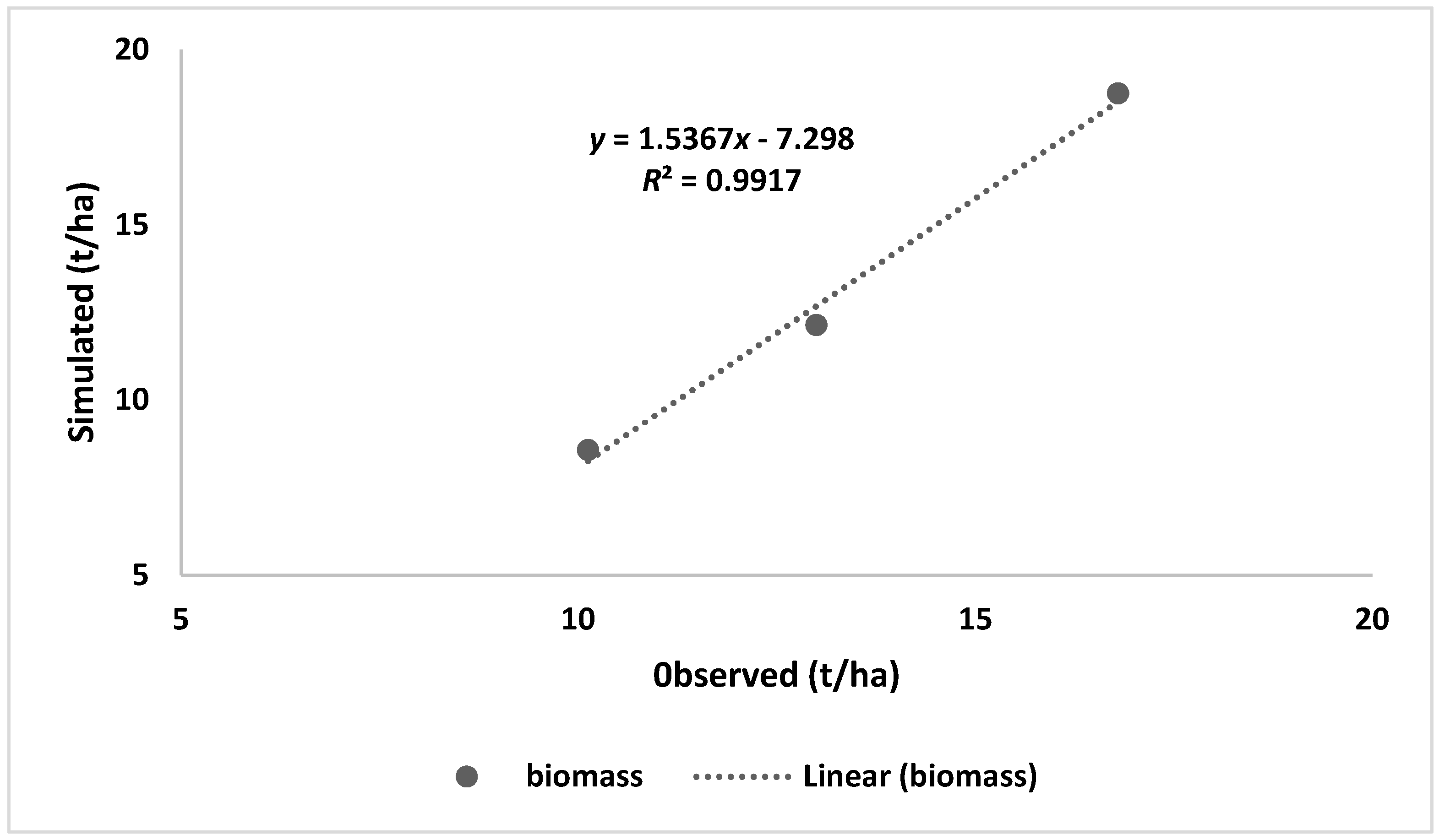
Figure 2.
Simulated vs. measured final grain yield for all three growing seasons.
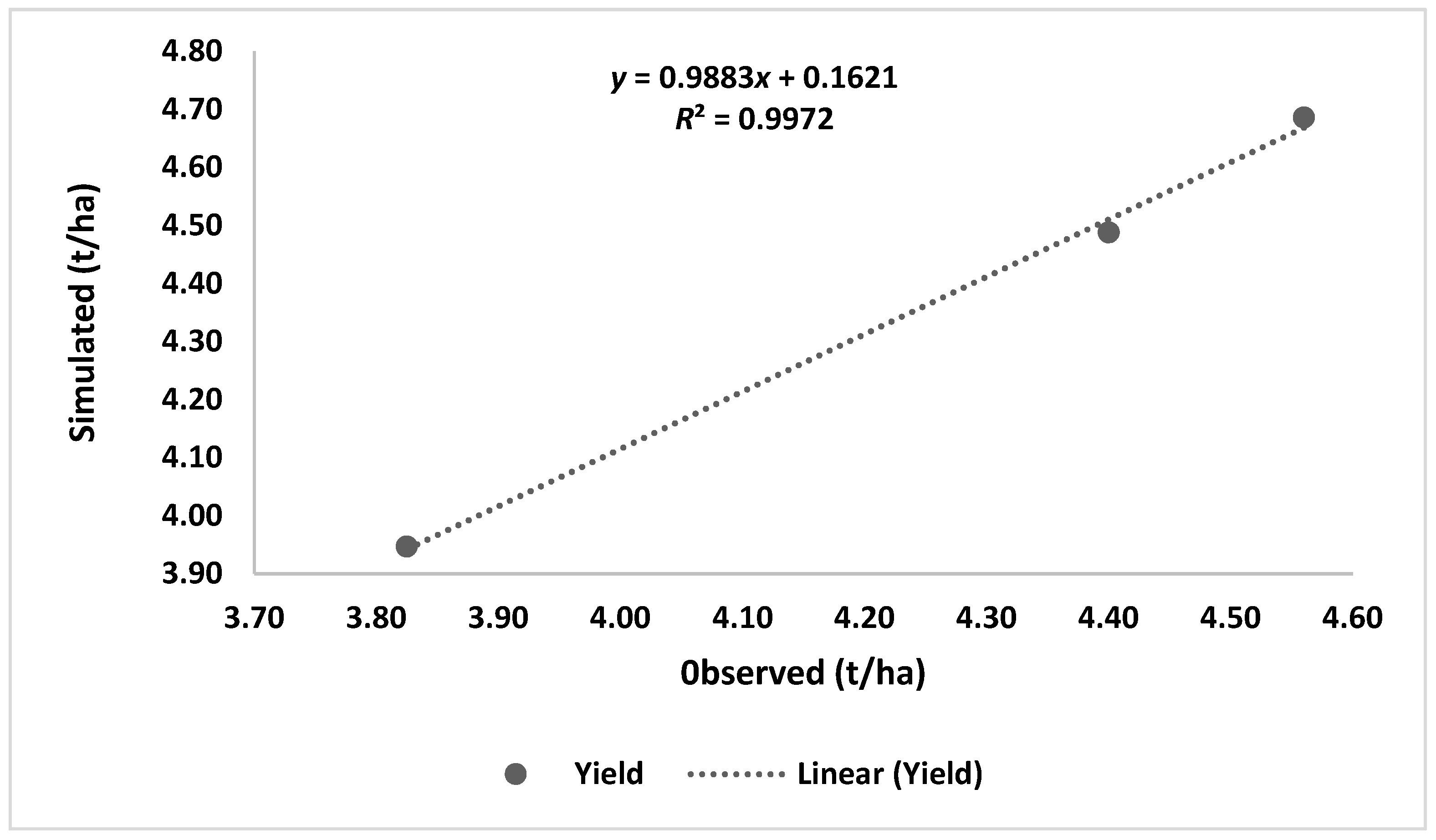
Figure 3.
Rainfall and evapotranspiration for the September to December 2015 growing season.

Figure 4.
Rainfall and evapotranspiration for the March to July 2015 growing season.

Figure 5.
Rainfall and evapotranspiration for the September to December 2014 growing season.


Table 1.
Experimental and agronomic data.
| Parameter | September to December 2014 | March to July 2015 | September to December 2015 |
|---|---|---|---|
| Plant population, plants ha−1 | 66,667 | 50,000 | 53,333 |
| Sowing date | 12 September 2014 | 25 March 2015 | 14 September 2015 |
| Harvest date | 24 December 2014 | 09 July 2015 | 29 December 2015 |
| Number of days from sowing to emergence | 7 | 6 | 6 |
| Number of days from sowing to flowering | 73 | 72 | 66 |
| Number of days from sowing to maturity | 104 | 107 | 107 |
| Seasonal rainfall, mm | 542 | 302 | 590 |
| Seasonal reference evaporation, mm | 555 | 519 | 691 |
| Average growing degree days, °C day | 1149 | 1145 | 1321 |
Table 2.
Soil properties of the study area.
| Depth (cm) | Sand % | Clay % | Silt % | pH | BD (g/cm3) | θpwp (%) | θfc (%) | θsat (%) | Ksat (cm/h) |
|---|---|---|---|---|---|---|---|---|---|
| 0–15 | 33 | 37 | 30 | 5.3 | 1.33 | 19 | 31 | 51 | 0.250 |
| 15–30 | 29 | 45 | 26 | 5.4 | 1.35 | 20 | 32 | 51 | 0.248 |
| 30–45 | 26 | 50 | 24 | 5.5 | 1.35 | 17 | 28 | 45 | 0.205 |
| 45–60 | 25 | 56 | 19 | 5.3 | 1.36 | 16 | 26 | 40 | 0.121 |
Table 3.
Conservative parameters used in the simulations.
| Parameter and Unit | Value |
|---|---|
| Base temperature, °C | 8.0 |
| Upper temperature, °C | 30.0 |
| Soil surface covered by an individual seedling at 90% emergence, (cm2/plant) | 6.5 |
| Canopy growth coefficient (CGC), % increase/day | 13 |
| Canopy decline coefficient (CDC), % decrease/day | 10 |
| Crop determinacy linked with flowering | Yes |
| Excess of potential fruits, % | 50 |
| Shape factor describing root zone expansion | 1.3 |
| Crop coefficient when canopy is complete but prior to senescence | 0.95 |
| Decline in crop coefficient after reaching maximum CC, % decline day−1 | 0.30 |
| Water productivity normalized for ETo and CO2, aWP* (g/m−3) | 33.7 |
| Water productivity normalized for ETo and CO2 during yield formation (as % WP* before yield formation) | 50 |
| Coefficient describing negative impact of stomatal closure during yield formation on Harvest Index | 3.0 |
| Possible increase (%) of Harvest Index due to water stress before flowering | None |
| Coefficient describing positive impact of restricted vegetative growth during yield formation on Harvest Index (HI) | Small |
| Coefficient describing negative impact of stomatal closure during yield formation on Harvest Index (HI) | Strong |
| Maximum possible increase in specified Harvest Index, % | 15 |
Table 4.
Canopy cover development for the September to December 2014 growing season.
| Date | Simulated Canopy (%) | Observed Canopy (%) | Deviation |
|---|---|---|---|
| 30 April | 0.33 | 0.63 | −0.3 |
| 1 May | 24.2 | 37.78 | −13.58 |
| 14 May | 71 | 79.96 | −8.96 |
| 30 May | 77.3 | 80.58 | −3.28 |
| 15 June | 72.9 | 77.98 | −5.08 |
| 9 July | 22.9 | 26.5 | −3.6 |
Table 5.
Measured vs simulated values of the final aboveground biomass and grain yield.
| Growing Season | Biomass (t/ha) | Grain Yield (t/ha) | ||||
|---|---|---|---|---|---|---|
| Measured | Simulated | Deviation(%) | Measured | Simulated | Deviation (%) | |
| September to December 2014 | 13.00 | 12.14 | −6.6 | 4.40 | 4.49 | 2.0 |
| March to July 2015 | 10.13 | 8.57 | −15.4 | 3.83 | 3.95 | 3.2 |
| September to December 2015 | 16.80 | 18.75 | 11.6 | 4.56 | 4.69 | −2.8 |
Table 6.
Statistical values for evaluating the performance of the AquaCrop model in simulations of final aboveground biomass and grain yield for all the three seasons.
Table 6.
Statistical values for evaluating the performance of the AquaCrop model in simulations of final aboveground biomass and grain yield for all the three seasons.
| Biomass | Grain Yield | |
|---|---|---|
| RMSE (t/ha) | 1.52 | 0.11 |
| E | 0.69 | 0.87 |
© 2018 by the authors. Licensee MDPI, Basel, Switzerland. This article is an open access article distributed under the terms and conditions of the Creative Commons Attribution (CC BY) license (http://creativecommons.org/licenses/by/4.0/).
Share and Cite
MDPI and ACS Style
Mibulo, T.; Kiggundu, N. Evaluation of FAO AquaCrop Model for Simulating Rainfed Maize Growth and Yields in Uganda. Agronomy 2018, 8, 238. https://doi.org/10.3390/agronomy8110238
AMA Style
Mibulo T, Kiggundu N. Evaluation of FAO AquaCrop Model for Simulating Rainfed Maize Growth and Yields in Uganda. Agronomy. 2018; 8(11):238. https://doi.org/10.3390/agronomy8110238
Chicago/Turabian StyleMibulo, Tadeo, and Nicholas Kiggundu. 2018. "Evaluation of FAO AquaCrop Model for Simulating Rainfed Maize Growth and Yields in Uganda" Agronomy 8, no. 11: 238. https://doi.org/10.3390/agronomy8110238
Note that from the first issue of 2016, this journal uses article numbers instead of page numbers. See further details here.