Selection of Appropriate Spatial Resolution for the Meteorological Data for Regional Winter Wheat Potential Productivity Simulation in China Based on WheatGrow Model

Abstract

The crop model based on physiology and ecology has been widely applied to the simulation of regional potential productivity. By determining the appropriate spatial resolution of meteorological data required for model simulation for different regions, we can reduce the difficulty of acquiring model input data, thereby improving the regional computing efficiency of the model and increasing the model applications. In this study, we investigated the appropriate spatial resolution of meteorological data needed for the regional potential productivity simulation of the WheatGrow model by scale effect index and verify the feasibility of using the landform to obtain the appropriate spatial resolution of meteorological data required by the potential productivity simulation for the winter wheat region of China. The research results indicated that the spatial variation of landforms in the winter wheat region of China is significantly correlated to the spatial variation of multi-year meteorological data. Based on the scale effect index, we can obtain a spatial distribution of appropriate spatial resolution for the meteorological data required for the regional potential productivity simulation of the WheatGrow model for the winter wheat region of China. Moreover, although we can use the spatial heterogeneity of landforms to guide the selection of appropriate spatial resolution for the meteorological data, in the regions where the spatial heterogeneity of the landform is relatively weak or relatively strong over a small range, the method of using a single heterogeneity index derived from semi-variogram cannot well reflect the scale effect of simulation results and needs further improvement.

1. Introduction

The potential productivity is the maximum production capacity of a variety when grown in environments to which it is adapted, with nutrients and water nonlimiting and with pests, diseases, weeds, lodging, and other stresses effectively controlled [1]. Regional potential productivity simulation can estimate characteristics of variation in the spatiotemporal distribution of crop productivity potential, identify the rule of variation in the upper limit of yield, optimize the planting system, and improve the use efficiency of agroclimatic resources, thereby providing a scientific reference for regional sustainable development [2,3]. At present, the simulation of the regional potential productivity of crops includes two methods: the empirical model and the mechanical model. The empirical model, often used includes the agro-ecological region method (AEZ) recommended by the United Nations Food and Agriculture Organization (FAO) [4,5]. However, the empirical model, which establishes a simple statistical equation based on statistical data, does not consider the genetic characteristics and growth and development of crops, and the interpretation and universality is relatively poor. The mechanical model is based on the eco-physiological process of crop growth and is a powerful tool to predict crop yield, manage agricultural resources, and assess the influence of climate change on agricultural production, and is most widely applied in the regional potential productivity simulation [6]. At present, the CERES-WHEAT model [7,8] WOFOST model [9,10] and WheatGrow model [11,12] of wheat growth have been applied to the simulation of the regional potential productivity in China.

However, the lack of high-quality spatial input data is the main problem for the regional simulation of the crop model [13]. One important method to solve this problem is to couple the crop model and GIS and use the spatial interpolation method to interpolate the station data of the model into a grid surface. Moreover, every homogeneous pixel (grid) is taken as a simulation unit for the model calculation, and therefore, the regional simulation yield is obtained [14]. As the model input data have spatial heterogeneity, using high spatial-resolution data will increase the difficulty of data acquisition and reduce the computational efficiency of the model [15,16]. Therefore, the issue of input data needs to be solved in the regional application of the crop model to analyze the scale effect of the simulation results and to determine the appropriate spatial resolution of the model input data based on the model input data of different spatial resolutions.

Meteorological data are the main input data for the regional potential productivity simulation. The use of high spatial resolution meteorological data for the regional potential productivity simulation can reflect more spatial details and ensure simulation accuracy, but increase the model computation and data storage. However, the use of low spatial resolution meteorological data will cause the loss of data information. Moreover, the stronger the spatial heterogeneity of meteorological data is, the more significant the loss of data information will be, which can cause a reduction in simulation accuracy [15,16,17,18,19,20]. Therefore, it has been widely suggested to study the influence of meteorological data with different spatial resolutions on the regional potential productivity simulation and to select the appropriate spatial resolution of meteorological data for the model simulation. Previous studies have conducted relevant regional studies and constructed a strategy to guide the selection of appropriate spatial resolution for meteorological data based on the spatial heterogeneity of landforms [15,16,21,22,23]. The winter wheat region of China is vast, and the climate conditions and ecological conditions are complicated. The WheatGrow model is the primary model for the simulation of potential productivity. Relevant studies on the influence of meteorological data with different spatial resolutions on the regional potential productivity simulation of the WheatGrow model have not been conducted, and the relationship between the spatial heterogeneity of landforms and the appropriate spatial resolution of the meteorological data has not been studied.

In this study, we take the winter wheat region of China as the research area and construct the multi-spatial resolution meteorological data. We use the WheatGrow model to simulate the regional potential productivity and construct the scale effect index to analyze the scale effect of simulation results. Moreover, we use the threshold of the scale effect index to determine the appropriate spatial resolution of the meteorological data needed for the simulation of potential productivity in the winter wheat region of China. Finally, we combine the relationship between the spatial heterogeneity of the landform and the scale effect index and investigate the feasibility of using the spatial heterogeneity of landforms to acquire the appropriate spatial resolution of meteorological data required for the potential productivity simulation in the winter wheat region of China.

This paper is organized into four parts. The material section (Section 2) describes the geographic overview of the research area and introduces the simulation model of crop growth used in this study, the data source, and the preconditioning. The method section (Section 2) describes the construction method of the scale effect index, the selection method for the appropriate spatial resolution of the meteorological data, and the method to analyze the spatial heterogeneity of the landform. The results and discussion section (Section 3) presents the simulation results for different spatial resolutions in the research area and the spatial distribution for the appropriate spatial resolution of meteorological data and the investigation on the relationship between the scale effect of the simulation results and the spatial heterogeneity of the landform. This section also investigates the feasibility of selecting the appropriate spatial resolution of meteorological data based on the spatial heterogeneity of the landform. Finally, we present the conclusions obtained by this study (Section 4).

2. Materials and Methods

2.1. Research Area

In this study, we took the winter wheat region of China as the research area (Figure 1a). The winter wheat region of China (102°46′–122°11′ E, 28°13′–41°10′ N) is the main production area of winter wheat in China. The region was divided into four sub-regions: The north winter wheat sub-region (NS), the Huang-Huai winter wheat sub-region (HHS), the middle-lower reaches of the Yangzi River winter wheat sub-region (MYS) and the southwest winter wheat sub-region (SWS) (Figure 1b). There were various climate types, including a middle temperature semiarid zone, a middle temperate semi-humid zone, a warm temperate semi-humid zone, a warm temperate semi-arid region, a north subtropical humid region, and a middle subtropical humid region [24]. The regional spatial distributions of light and temperature resource conditions and terrain have strong characteristics of spatial variability (Figure 1c–e), and the difference in temperature and precipitation was relatively significant. In particular, the annual average temperature in the NS and HHS is 9–15 °C, and the annual precipitation was 440–980 mm; the annual average temperature in the MYS and SWS was 16–25 °C, and the annual precipitation was typically above 1000 mm [25]. The landforms in the winter wheat region include plains, hills, mountains, and basins, and the difference between the elevation in the east and west was significant. The highest elevation was 5174 m, and the lowest elevation was −142 m (Figure 1c).

2.2. WheatGrow Model

The process-based WheatGrow model has been widely applied to regional potential productivity simulations in China [11,12,26]. This model includes five sub-models: Apical development and phenology [27,28,29]; photosynthesis and dry matter production [12]; material distribution and organogenesis [27,30]; yield and quality formation [31,32]; and soil moisture and nutrient balance [33,34]. The model runs at a daily time step, simulating wheat growth and development under potential production, water-limited and nitrogen-limited scenarios [31,35]. The WheatGrow model has been validated through simulation at multiple eco-sites and under different scales in the main yield region of winter wheat in China, and the results indicate that this model can simulate and predict the growth and development of wheat and the yield formation [36,37].

2.3. Data Description

The simulation of potential productivity is not subject to the restriction of water, nitrogen, and soil conditions, and is only subject to the influence of weather, variety parameters, and sowing date [38,39,40]. The meteorological data include daily maximum temperature (Tmax), daily minimum temperature (Tmin), and sunshine duration (SSD). The daily data at 982 meteorological stations in the winter wheat area during 2000–2009 were obtained through the meteorological scientific data sharing service of China Meteorological Administration (http://cdc.nmic.cn/home.do) (Figure 1b). We used the ANUSPLIN local thin plate smooth spline method to interpolate the daily meteorological data in the research area into the multi-resolution grid data [41]. By using the resolution range from 1 km to 200 km adopted in previous studies [15,18,42], we constructed the nested sequence of spatial resolution l_i (i = 0, 1, 2, 3, 4, 5) as l₀ = 5 km, l₁ = 10 km, l₂ = 20 km, l₃ = 40 km, l₄ = 80 km, and l₅ = 160 km. To restrict the influence of variety parameters and sowing date on this study, our study uses the same set of variety parameters of the regional typical winter wheat (Triticum aestivum L.) cultivar Ningmai 13 (

Table 1. Variety parameters adopted by the WheatGrow model in this study.

Name	Description	Unit	Value
PVT	Physiological vernalization time	d	12
IE	Intrinsic earliness	-	0.85
PS	Photoperiod sensitivity	-	0.0008
TS	Temperature sensitivity	-	1.1
FDF	Filling duration factor	-	0.8
HI	Harvest index	-	0.42
LT	Thermal time between two successive leaf tip appearances	°C·d	66
GW	1000-grain weight	g	39.3
SLA	Specific leaf area under optimum conditions	ha kg−1	0.002
TA	Tilling ability	-	0.87

) and sets the sowing date uniformly as the 261st day of every year [15]. The terrain data in the study adopt the SRTMGL1_003 DEM data with a spatial resolution of 30 m [43]. Moreover, we use the NEAREST (nearest neighbor assignment) grid re-sampling method to obtain the DEM data with a spatial resolution of l₀ [44].

2.4. General Workflow of Analysis

In this study, by constructing the scale effect index S, we analyze the influence of meteorological data with six spatial resolutions on the regional potential productivity simulation of WheatGrow in the winter wheat area of China over 10 years (2000–2009) and adopt the threshold of the scale effect index S to determine the appropriate spatial resolution ASRS of the meteorological data required for the regional potential productivity simulation in the research area. Meanwhile, we analyze the semi-variogram of the DEM and use the relationship between the scale effect index S and the sill value ς of the DEM semi-variogram to obtain the appropriate spatial resolution ASR^ς of meteorological data based on the spatial heterogeneity of the landform. With the range of semi-variogram, we also compare the results of the two methods and evaluate the influence of landform spatial heterogeneity on the distribution of regional light and temperature resources as well as the effect and feasibility of using the spatial heterogeneity of the landform to obtain the appropriate spatial resolution of meteorological data required for the regional potential productivity simulation of WheatGrow (Figure 2).

2.5. Construction of the Scale Effect Index

In this study, based on the method of spatial gradient analysis, we designed the scale effect index S with the statistical root-mean-square error (RMSE) between the pixels of different spatial resolutions as the basis [45] and quantitatively reflect the difference between the simulation results of spatial resolution l_i (i > 0) and the highest spatial resolution l₀ caused by the change in the spatial resolution of the meteorological data. The scale effect index S is shown in Equation (1):

$$S={(n^{-1}{\displaystyle \sum _{c=1}^n{\overline{\Delta Y_c}}^2})}^{1/2}$$

(1)

where n is the number of pixels with spatial resolution l₀ contained in one pixel of meteorological data with spatial resolution l_i (i > 0).

$$\overline{\Delta Y_c}=\overline{YL}-\overline{Y{H}_c}$$

(2)

$\overline{YL}$ and $\overline{Y{H}_c}$, respectively, represent the 10-year average value of simulation results with spatial resolutions of l_i (i > 0) and l₀ for the meteorological data,

$$\overline{YL}=({\displaystyle \sum _{y=1}^{y=10}Y{L}_y})/10$$

(3)

$$\overline{Y{H}_c}=({\displaystyle \sum _{y=1}^{y=10}Y{H}_{c,y}})/10$$

(4)

YL_y and YH_c,y represent the simulation results of regional potential productivity in the yth year.

$$Y{L}_y=f(W_{l_i,y})(i>0)$$

(5)

$$Y{H}_{c,y}=f(W_{l_0,y})$$

(6)

where f represents the crop model, YL_y represents the simulation result obtained using the meteorological data $W_{l_i,y}(i>0)$ with spatial resolution l_i (i > 0) in the yth year, and YH_c,y represents the simulation results obtained using the meteorological data $W_{l_0,y}$ with spatial resolution l₀ in the yth year.

2.6. Analysis of the Characteristics of Terrain Spatial Variation Based on the Semi-Variogram

The landform is an important factor that affects the simulation of the regional potential productivity of crops [46,47]. The expression of terrain data has relatively strong characteristics of scale dependence, and its spatial heterogeneity has a significant influence on the scale effect for the simulation results of regional potential productivity [15]. In this study, we analyzed the semi-variogram of the DEM and use the sill value ς of the semi-variogram to characterize the spatial heterogeneity of the landform [48].

The semi-variogram γ(h) is the function used to evaluate the autocorrelation of the spatial process and is defined as half of the variance for the difference in regional variable Z(x) at points x and x + h, Z(x) and Z(x + h):

$$\gamma (h)=\frac{1}{2N(h)}{{\displaystyle \sum _{i=1}^{N(h)}\left[Z(x_i)-Z(x_i+h)\right]}}^2$$

(7)

There are several theoretical models of semi-variogram including Spherical, Exponential, Gaussian, etc. [49]. In this study, the DEM semi-variogram is fitted with the spherical model and the spatial distribution of the pixel values was assumed isotropic [15,50,51]. The Spherical model is as follows:

$$\gamma (h)=\{\begin{array}{cc}{C}_0\hfill & \hfill h=0\\ C_0+C(\frac{3h}{2a}-\frac{h^3}{2a^3})\hfill & \hfill 0<h\le a\\ \varsigma \hfill & \hfill h>a\end{array}$$

(8)

where C₀ is the nugget constant; ς = C₀ + C is the sill value of the semi-variogram, where the larger the value of ς is, the stronger the spatial variability of the landform; a is the range, namely, the distance for the value of the DEM semi-variogram to reach the sill value; and h is the distance [49]. When the samples are located on a regular grid, the distance between two points should be smaller than half the grid extent to ensure the significance of the semi-variogram [52]. So in this study, the maximum distance to compute the semi-variogram was set to 1/3 of the grid extent when the spatial resolution is l_i (i > 2) [52,53]. Because the DEM with spatial resolution l₀ nested in each grid is relatively few when the spatial resolution is l_i (i = 1,2), the maximum distance was respectively set to 10 km and 20 km to fit the semi-variogram properly.

2.7. Selection of Appropriate Spatial Resolution for the Meteorological Data of Regional Potential Productivity Simulation

In this study, we adopted the scale effect index S and the sill value ς of the DEM semi-variogram to quantitatively reflect the influence of the spatial resolution of the meteorological data on the simulation results. To use the multi-spatial resolution data fusion method to obtain the spatial distribution for the appropriate spatial resolution of meteorological data, in this study, we set the threshold for the scale effect index S(l_i) (i > 0) of the simulation results with spatial resolution l_i (i > 0) to be t. If S(l_i) ≤ t, in comparison with using the data with spatial resolution l_i (i > 0), the application of meteorological data with spatial resolution l₀ has limited capability to increase the accuracy of regional potential productivity simulation. We can use the grid with spatial resolution l_i (i > 0) to replace the grid with spatial resolution l₀ for the regional potential productivity simulation and therefore reduce the computational load of the model when the spatial resolution l_i (i > 0) is the appropriate spatial resolution. If S(l_i) > t, we abandon the replacement operation. The value of i successively traverses from 1 to 5, and eventually, we can obtain the appropriate spatial resolution ASR^S of meteorological data required by the regional potential productivity simulation.

Meanwhile, taking the grid with spatial resolution l_i (i > 0) in the research area as the region, we analyzed the semi-variogram of the DEM with spatial resolution l₀ nested in each grid and eventually obtain the spatial distribution for the sill value ς of the DEM semi-variogram with spatial resolution l_i (i > 0). Under spatial resolution l_i (i > 0), we fit the relationship ln(S)~ln(ς) between the natural logarithmic value of the sill value ς of the DEM semi-variogram and the scale effect index S. Therefore, according to the threshold of scale effect index S, we can obtain the threshold for the sill value ς of the DEM semi-variogram. By adopting the aforementioned method, we can obtain the appropriate spatial resolution ASR^ς of the meteorological data based on the threshold for the sill value ς of the DEM semi-variogram.

3. Results and Discussion

In this study, we used the WheatGrow model to obtain the simulation results of potential productivity during the 2000–2009 seasons for the winter wheat region of China (Figure 3). The regional difference in the simulation results of potential productivity is significant. The average level of potential productivity in the NS and HHS is relatively high: 8660.7 kg ha⁻¹ year⁻¹ (Figure 4b) and 8229.2 kg ha⁻¹ year⁻¹, respectively (Figure 4c). The high value regions are primarily distributed in the regions of the Loess Plateau, Shanxi middle mountains and basins, and Ludong low hills (Figure 1c), followed by the MYS and the SWS. The productivity is 7673.6 kg ha⁻¹ year⁻¹ in the MYS (Figure 4d) and 7612.2 kg ha⁻¹ year⁻¹ in the SWS (Figure 4a). The high-value areas are distributed in the regions of the southwest Sichuan-Central Yunnan subalpine mountains and basins and Qinling-Daba subalpine mountains, and the low values are distributed in the regions of the Sichuan basin and middle reaches of the Yangzi River hilly plains (Figure 1c).

In addition, the simulation results of different spatial resolutions have a significant scale effect. As the spatial resolution changes, the spatial trend of the simulation results is essentially consistent, but the difference in the spatial details of the simulation results is obvious (Figure 3). As the spatial resolution of the meteorological data decreases, the maximum and minimum of the simulation results decrease, and the variation in the distribution difference of the simulation results is significant. In particular, the effect is most obvious in the SWS, NS, and HS (Figure 4).

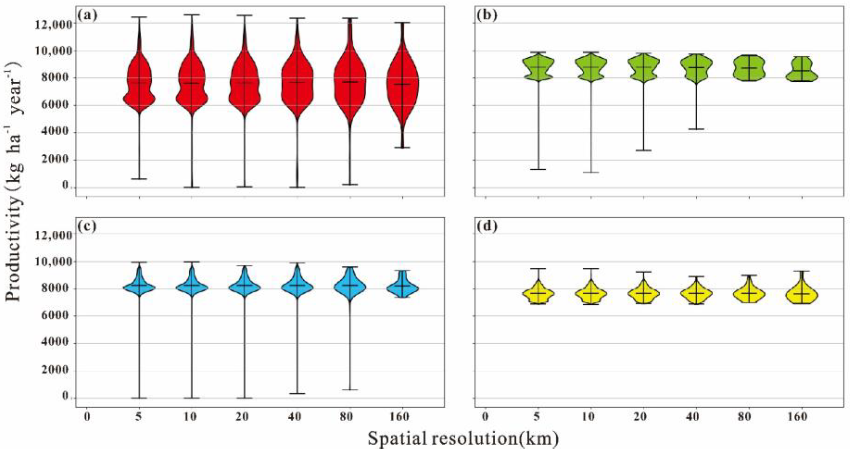
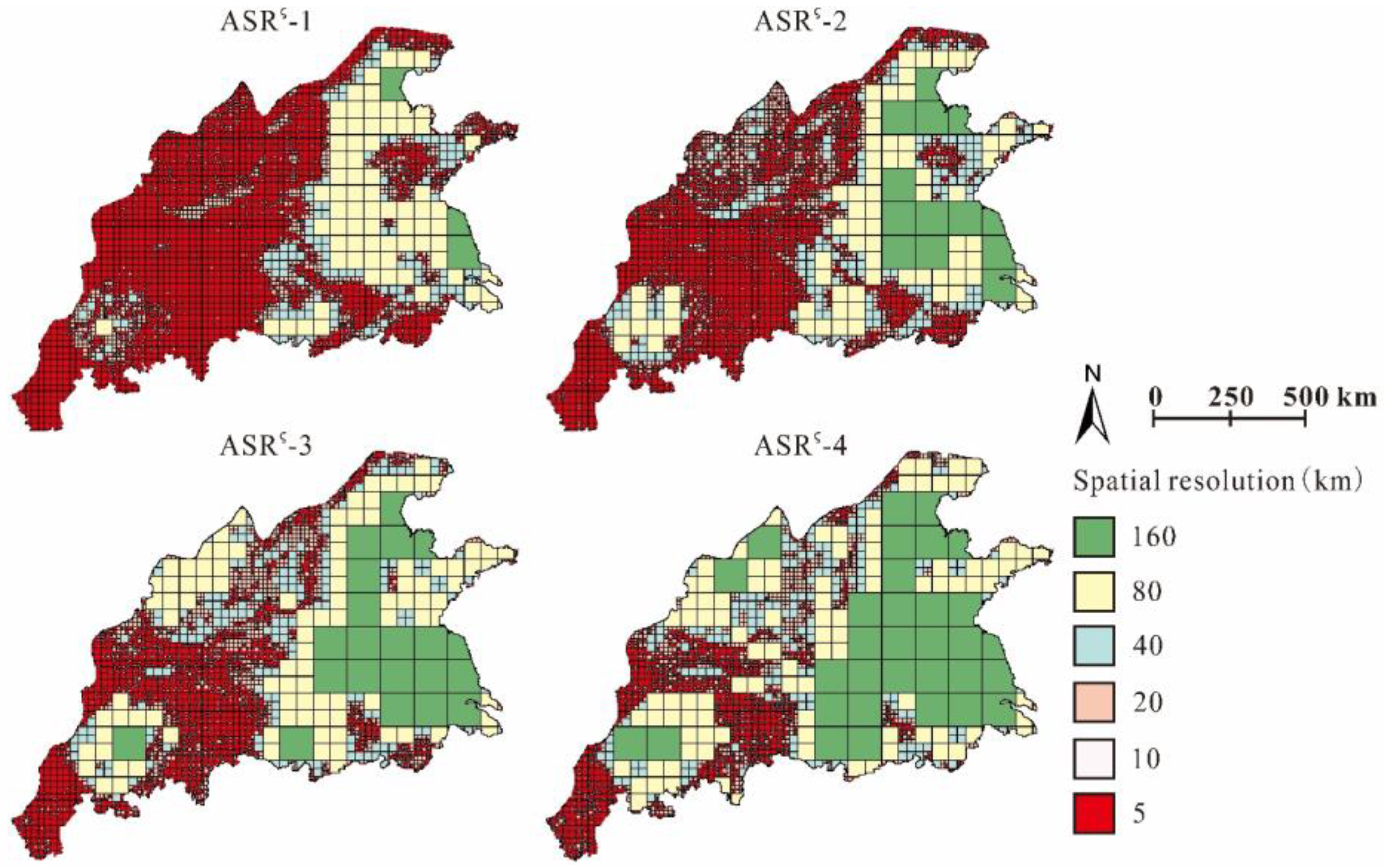
3.1. Selection of Appropriate Spatial Resolution Based on the Scale Effect Index

The spatial difference in the scale effect index S of the simulation results with different spatial resolutions is significant (Figure 5). The high values are primarily distributed in the regions with relatively strong spatial heterogeneity of landforms in the west of the research area, and the low values are primarily distributed in the eastern plains area. With the scale effect index S using the spatial resolution of 20 km as an example, the highest value that can be reached is e^9.04 ≈ 8433.8 kg ha⁻¹ year⁻¹, and the lowest value is only e^1.1 ≈ 3 kg ha⁻¹ year⁻¹. Furthermore, in the eastern plains area, the scale effect index S has the trend of gradually increasing as the spatial resolution of meteorological data declines.

We set the threshold of the scale effect index S as 100 kg ha⁻¹ year⁻¹, 200 kg ha⁻¹ year⁻¹, 300 kg ha⁻¹ year⁻¹, and 400 kg ha⁻¹ year⁻¹ and obtained the appropriate spatial resolution of meteorological data required for the regional potential productivity simulation of WheatGrow (Figure 6). The spatial resolution of data needed for the plains area in the east region of the research area is relatively low and is concentrated at 80 km and 160 km; the spatial resolution of data needed in the western and southwestern mountainous regions is relatively high, and is 5 km in most regions. As the threshold of scale effect index S increases, the spatial resolution in the most eastern plains area declines to 160 km and is maintained at 5 km in most regions with relatively strong spatial heterogeneity of landforms in the SWS.

The main purpose of this study was to construct the scale effect index S and to obtain the appropriate spatial resolution of meteorological data for the simulation of regional potential productivity in the winter wheat region of China in the allowed error range. Therefore, we can use the appropriate spatial resolution to effectively reduce the computations required by the model and decrease the difficulty in obtaining high-accuracy model input spatial data. In the regional application of the crop model, every grid is the basic simulation unit, and the number of grids represents the computational sum of the model [21,54]. In comparison with using the 5 km resolution meteorological data for the regional potential productivity simulation, the application of appropriate spatial resolution can effectively reduce the number of grids (Figure 7). Moreover, in the region in the eastern research area, where the spatial heterogeneity of the landforms is relatively weak, as the threshold of scale effect index S increases, the spatial resolution of the data changes to 160 km, and the number of grids decreases significantly; in the SWS with relatively strong spatial heterogeneity of landforms, the spatial resolution is maintained at 5 km, and the magnitude of the variation in the grid number is relatively small (Figure 6 and Figure 7).

Meanwhile, in this study, we selected the average value as the accuracy index to evaluate the use of the appropriate spatial resolution for the simulation [16,21]. In comparison with the average of simulation results with a spatial resolution of 5 km, the average of simulation results with appropriate spatial resolutions of ASR^S-1, ASR^S-2, ASR^S-3, and ASR^S-4 does not change considerably within a certain range, and the lowest absolute difference from the average of simulation results with a 5 km resolution can reach 5.2 kg ha⁻¹ year⁻¹ (

Table 2. Absolute difference between the average simulation results for the grids of different appropriate spatial resolutions and the average simulation results for the grid with a resolution of 5 km.

	Regions	Spatial Resolution
		5 km	ASRS-1	ASRS-2	ASRS-3	ASRS-4
Mean (kg ha−1 year−1)	Research area	8052.2	8132.5	8078.0	8037.3	8047.0
	SWS	7583.0	7752.7	7905.2	7963.1	8048.4
	NS	8758.3	8901.4	8706.6	8492.2	8288.8
	HHS	8220.0	8427.0	8410.7	8266.4	7957.8
	MYS	7641.1	7711.2	7821.2	7836.6	7765.2
Abs a (kg ha−1 year−1)	Research area	-	80.3	25.8	14.9	5.2
	SWS	-	169.7	322.2	380.1	465.4
	NS	-	143.1	51.7	266.1	469.5
	HHS	-	207	190.7	46.4	262.2
	MYS	-	70.1	180.1	195.5	124.1

^a Abs, the absolute difference between the appropriate spatial resolution of meteorological data used in different sub-regions and the average simulation results with a 5 km resolution.

). By using the appropriate spatial resolution for the simulation, we can ensure simulation accuracy, but for the SWS with relatively strong spatial heterogeneity of landforms, the average exhibits a trend of increasing as the threshold of scale effect index S increases.

Previous studies that obtained the appropriate spatial resolution of model input data as a single value [21], such as 100 km [16,19]. In this study, we used the multi-spatial resolution grid fusion method to optimize the data of unified spatial resolution and collect the appropriate spatial resolutions required for the regional potential productivity simulation on the same map (Figure 6). This approach can truly reflect the spatial distribution of resolution for meteorological data under different terrain backgrounds and solves the problem that the unified spatial resolution is not applicable to regions with relatively large differences in the spatial heterogeneity of landforms [19]. Therefore, it can satisfy the demand of various sub-regions in the winter wheat area of China at different appropriate spatial resolutions.

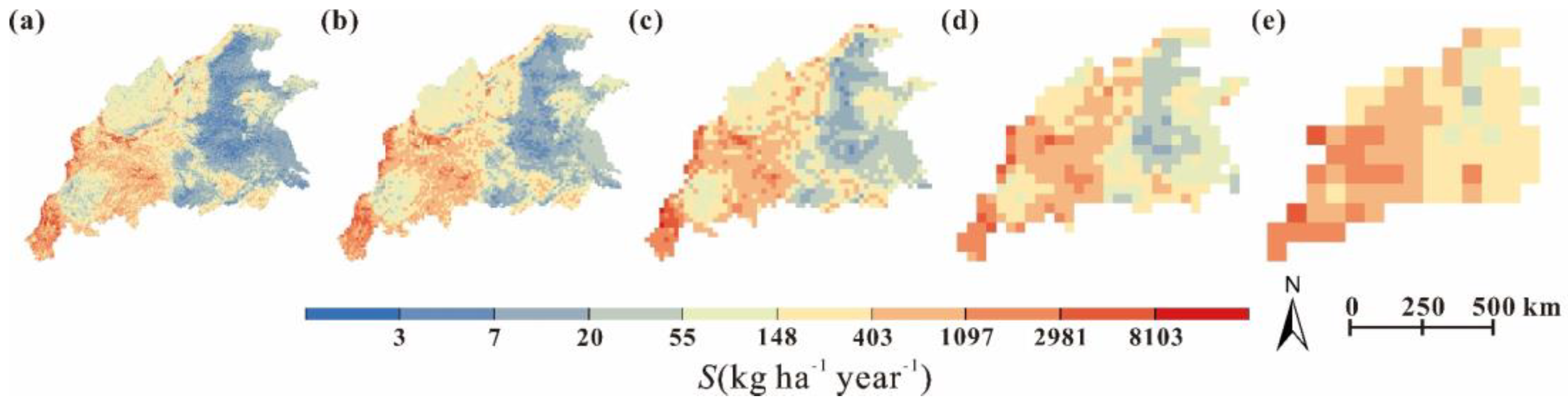
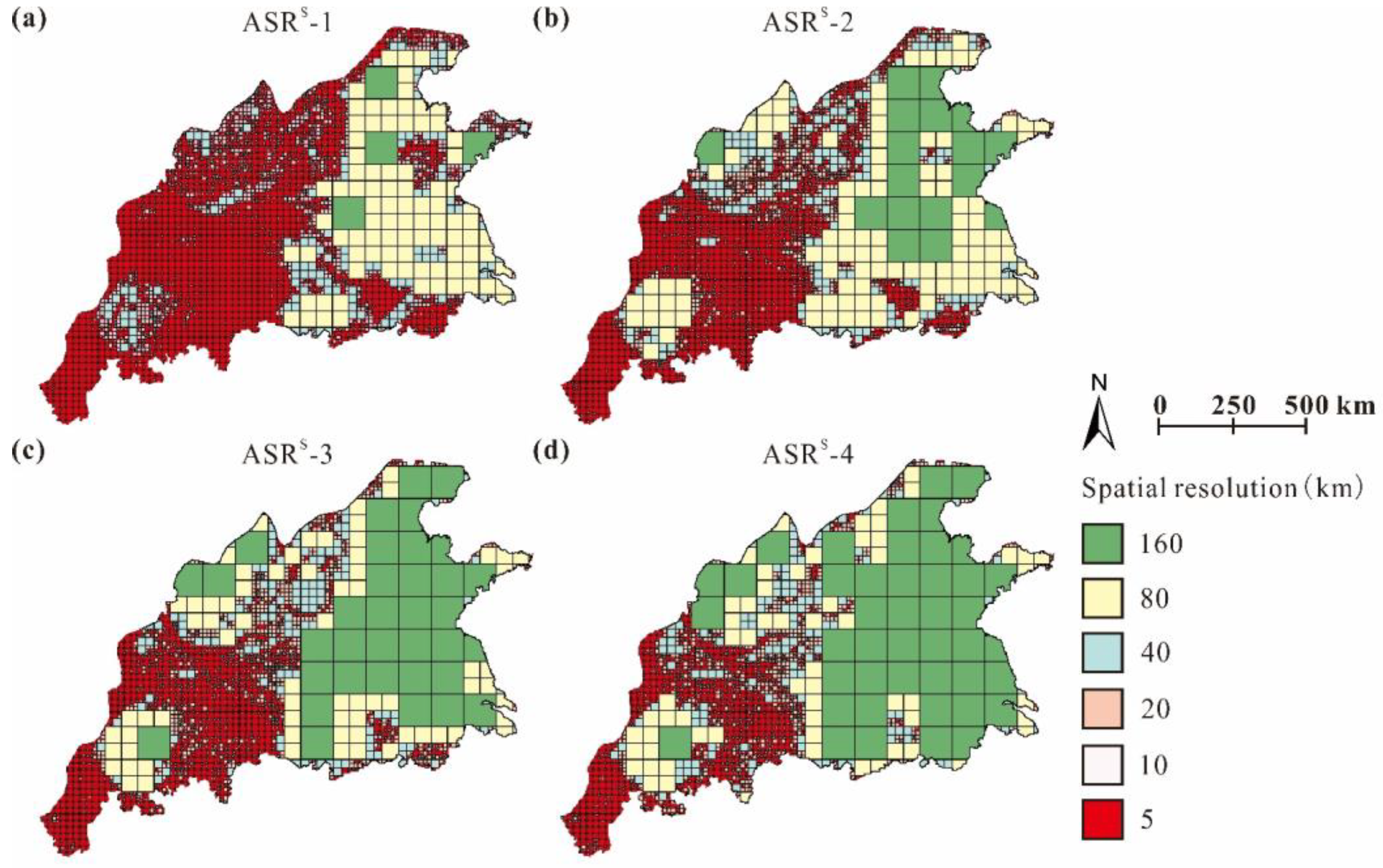
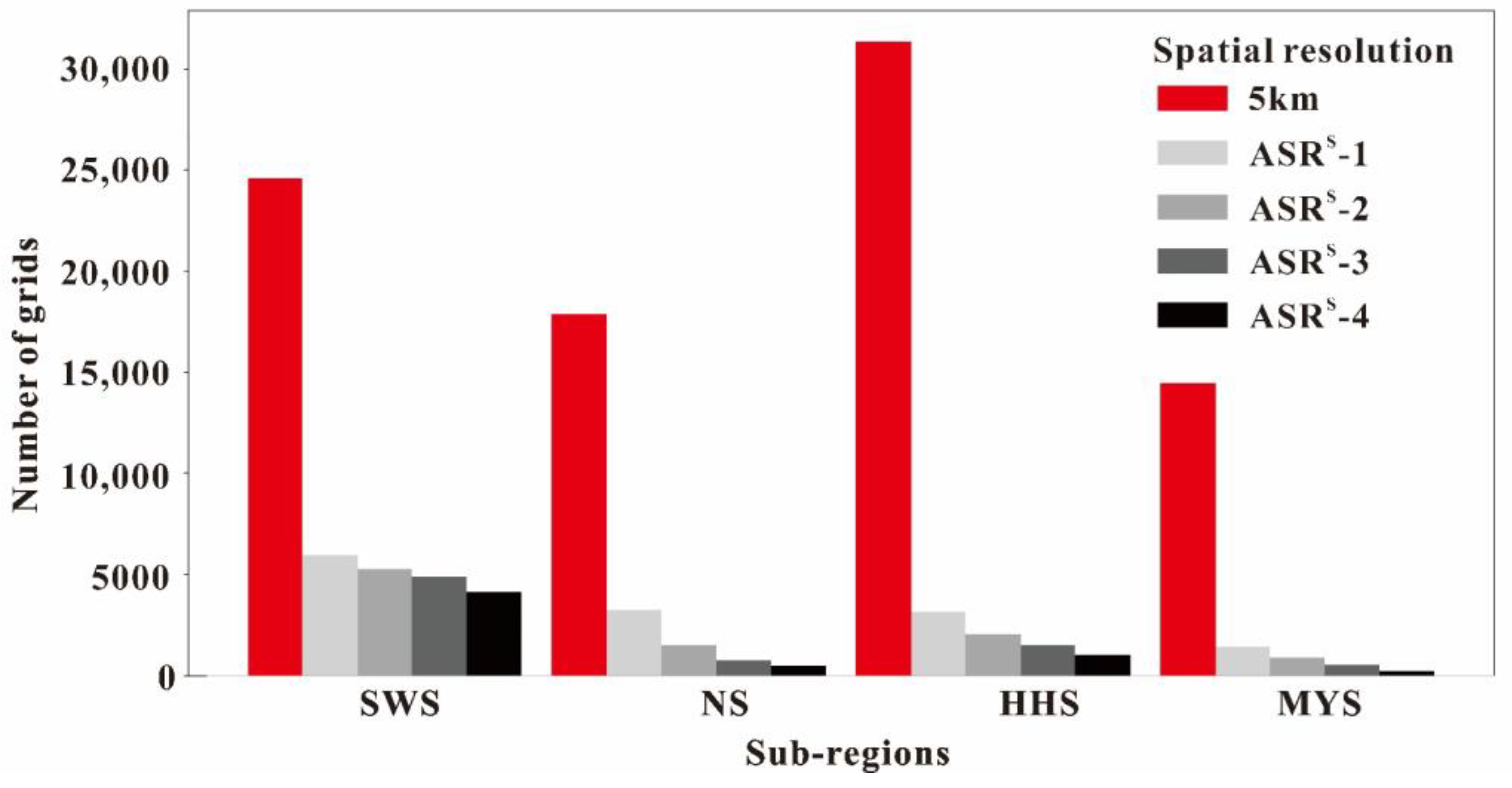
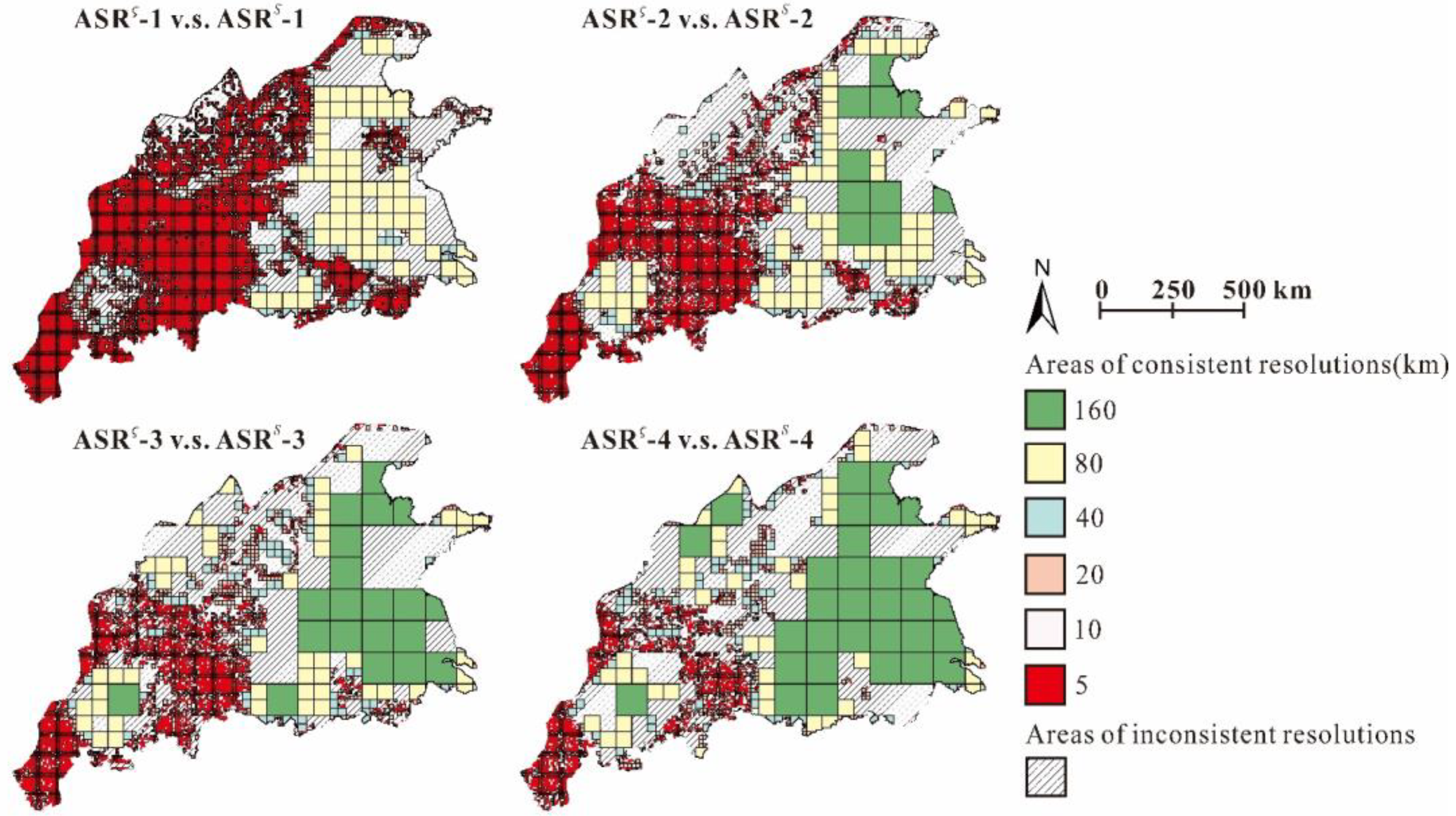
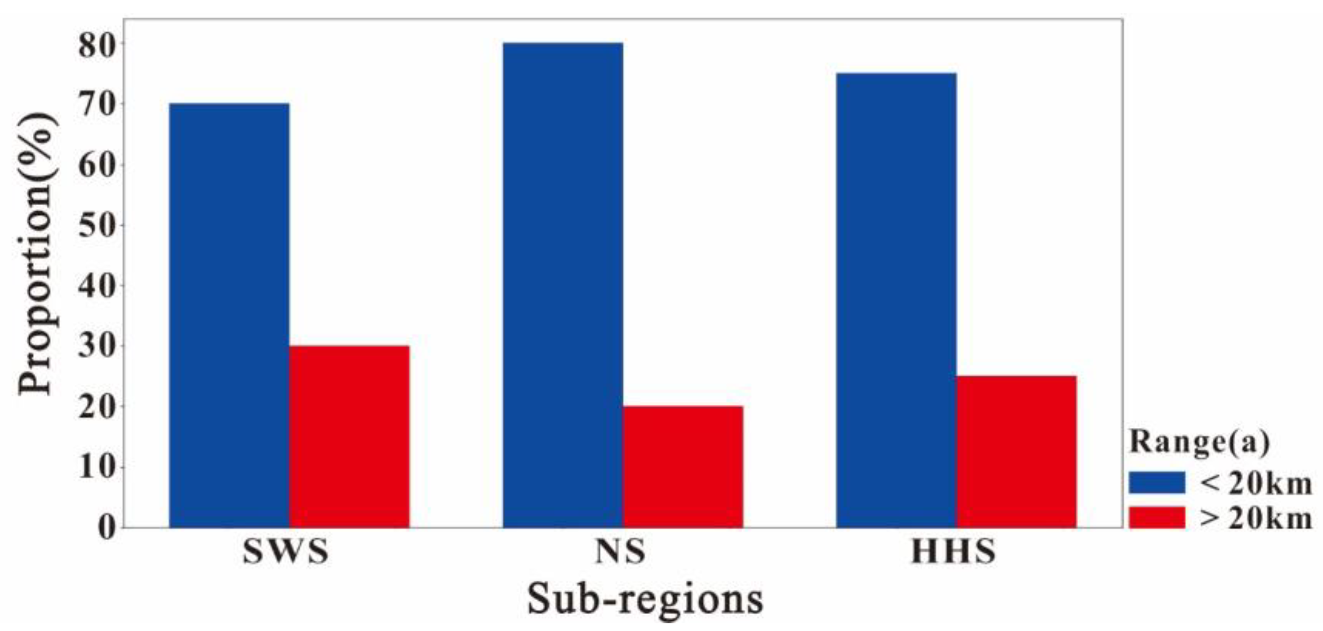
3.2. Selection of the Appropriate Spatial Resolution Based on the Spatial Heterogeneity of Landforms

Previous studies indicated that meteorological data are significantly affected by terrain, and we can use the spatial heterogeneity of landforms to reflect the scale effect of simulation results for the regional potential productivity [15,55,56]. In the region where the spatial heterogeneity of landforms is stronger, the larger the sill value ς of the DEM semi-variogram is, the larger the scale effect index S will be. The sill value and scale effect index exhibit a similar trend of spatial distribution (Figure 5 and Figure 8), and there is a significant correlation (Figure 9). As the spatial resolution decreases, the fitting relationship between the sill value ς of the DEM semi-variogram and the scale effect index S gradually weakens (Figure 9). By using the fitting relationship ln(S)~ln(ς), we obtained the threshold corresponding to the sill value ς of the DEM semi-variogram according to the threshold of the scale effect index S (

Table 3. Threshold setting for the sill value ς of the DEM semi-variogram.

Thresholds of S a (kg ha−1 year−1)	Thresholds of ς b (m2)
	10 km	20 km	40 km	80 km	160 km
100	5766	1762	1095	911	23
200	31,189	9608	7520	7619	601
300	83,727	25,918	23,214	26,399	4017
400	168,714	52,406	51,652	63,750	15,815

^a Thresholds of S reflect the threshold of scale effect index S. ^b Thresholds of ς reflect the threshold for the sill value ς of the DEM semi-variogram.

) and obtained the appropriate spatial resolution of the meteorological data based on the threshold for the sill value ς of the DEM semi-variogram (Figure 10).

By comparing the distribution of appropriate spatial resolution of meteorological data obtained by two methods, the Kappa coefficient in the SWS, HHS, and MYS was between 0.4 and 0.7 at a confidence level of α = 0.05. This indicates that the distribution of appropriate resolution from the two schemes has moderate, but not high, consistency (Figure 11 and

Table 4. Kappa consistency test of the appropriate spatial resolution obtained by the threshold of scale effect index S and the threshold for the sill value ς of the DEM semi-variogram: Southwest winter wheat sub-region (SWS), north winter wheat sub-region (NS), Huang-Huai winter wheat sub-region (HHS), and middle-lower reaches of the Yangzi River winter wheat sub-region (MYS).

Regions	Kappa Coefficient (p < 0.05)
	ASRς-1 vs. ASRS-1	ASRς-2 vs. ASRS-2	ASRς-3 vs. ASRS-3	ASRς-4 vs. ASRS-4
Research area	0.577	0.521	0.524	0.516
SWS	0.613	0.618	0.562	0.438
NS	0.3	0.253	0.238	0.322
HHS	0.574	0.506	0.466	0.521
MYS	0.55	0.463	0.635	0.566

) [57]. This is primarily because the spatial heterogeneity of meteorological factors in the research area cannot be completely expressed with the spatial heterogeneity of landforms, and the meteorological factors are still affected by the factors of longitude, latitude, and distance from the sea [58,59]. Furthermore, the scale of spatial heterogeneity for the terrain data and the spatial heterogeneity of the meteorological data is not united [59]. When the scale effect index S is relatively small, the ln(S)~ln(ς) fitting relationship exhibits an aggregation phenomenon (Figure 9, rectangle); when the scale effect index S is relatively large, the ln(S)~ln(ς) fitting relationship exhibits a saturation phenomenon (Figure 9, ellipse). With the spatial resolution of 20 km as an example, when ln(ς) < 4, there is no significant correlation between ln(S) and ln(ς) for the NS, HHS, and MYS (Figure 12b–d). At this popint, the sill value of the DEM semi-variogram is ς < e⁴ ≈ 55 m², which indicates that this region is primarily distributed in the eastern plains region of research area (Figure 8), and the spatial heterogeneity of the landform is weak. Therefore, for the regions with relatively weak spatial heterogeneity of landforms, the application of terrain cannot reflect the scale effect for the simulation results of potential productivity; meanwhile, when ln(ς) > 10, as ln(S) increases, ln(ς) no longer increases according to the fitting relationship (Figure 12, ellipse). In these regions, the variation range of the topographic semi-variogram is smaller than the spatial resolution of the grid at more than 70% of the grid points (Figure 13). That is, when the spatial variation of landforms occurs in a relatively small range, the spatial variation of landforms cannot reflect the scale effect for the simulation results of potential productivity and cannot guide the selection of appropriate spatial resolution in this region.

In this study, we adopted spatial semi-variogram analysis to describe the spatial heterogeneity of natural factors with an isotropic model [60,61]. However, semi-variogram analysis relies on the selected theoretical semi-variogram model as well as the direction, and the incorrect selection of the theoretical semi-variogram model or ignorance of anisotropy can lead to results for the characteristic spatial variation of landforms that are difficult to interpret. Meanwhile, the lag distance, range, and sill value in the semi-variogram analysis often affect each other, causing unstable analysis results and therefore affecting the results of this study [62]. It is important to combine multiple parameters for the semi-variogram analysis to obtain more reliable results [63]. In addition, although the appropriate spatial resolution obtained in this study can significantly reduce the computational load of regional potential productivity simulation under the requirement of ensuring accuracy, it is limited by the resolution sequence constructed in this study rather than the so-called global optimum spatial resolution. Meanwhile, there is not a scale (resolution) that is appropriate for the studies on all the geographic processes involved in the regional application of the crop model [64]. Its suitability is manifested by the matching of the crop growth simulation model and virtual geographical environment representation with respect to the domains of issue, structure, and dimension. By selecting the appropriate resolution from the limited resolution sequence, we can reduce the influence of resolution on the accuracy and efficiency of simulation results.

Moreover, this study is constrained to potential productivity simulation with WheatGrowth model. And land productivity simulation, rather than potential productivity simulation, is more vulnerable to the variability of soil [16,65]. Besides, it is also found that the uncertainties of radiation and precipitation have little influence over the regional yield forecast with World Food Studies (WOFOST) crop simulation model [21]. These issues indicate the range of model limitations and specificities of crop model applications [66], and should be focused and studied in our future researches.

4. Conclusions

In this study, we took the winter wheat region of China as the research area and simulated the regional potential productivity from 2000 to 2009 based on the WheatGrow model by constructing meteorological data with six spatial resolutions. We analyzed the influence of the scale effect for the meteorological data on the simulation of potential productivity in the winter wheat region of China and obtained the appropriate spatial resolution of meteorological data for the regional potential productivity simulation. Moreover, we clarified the feasibility of using the topographic features to obtain the appropriate spatial resolution of meteorological data required for the simulation of potential productivity in the winter wheat region of China. (1) Based on the threshold of the scale effect index, through multi-spatial resolution grid data fusion, we can effectively obtain the appropriate spatial resolution of the meteorological data required by the regional potential productivity simulation in the winter wheat area of China. The spatial resolution of data needed for the eastern plains area is relatively low, and it is concentrated at 80 km and 160 km; the spatial resolution of data needed for the western and southwestern mountainous and hilly regions is relatively high, and it is concentrated at 5 km. (2) The stronger the spatial heterogeneity of the topographic environment and meteorological environment is, the higher the spatial resolution of meteorological data required for the regional potential productivity simulation, and vice versa. (3) By using the appropriate spatial resolution of meteorological data to conduct the regional potential productivity simulation, we can ensure simulation accuracy, reduce the amount of regional simulation units, increase the efficiency of regional simulation, and improve the capability of explaining the spatial morphology and differences in the results of simulation of the regional potential productivity. (4) Although the application of the sill value for the DEM semi-variogram can guide the selection of the appropriate spatial resolution for the meteorological data, in the regions with relatively weak spatial heterogeneity of landforms on the eastern plains or the small-scale regions with strong spatial variation of landforms in the southwest, it cannot sufficiently reflect the scale effect for the simulation results of potential productivity. Therefore, the application is restricted to using the single heterogeneity index of landforms to obtain the appropriate spatial resolution of meteorological data required for the regional potential productivity simulation of winter wheat in China and needs further improvement.

References

1. Lloyd, T.E. Crop Evolution, Adaptation and Yield; Cambridge University Press: Cambridge, UK, 1996. [Google Scholar]
2. Gustafson, D.I.; Jones, J.W.; Porter, C.H.; Hyman, G.; Edgerton, M.D.; Gocken, T.; Shryock, J.; Doane, M.; Budreski, K.; Stone, C. Climate adaptation imperatives: Untapped global maize yield opportunities. Int. J. Agric. Sustain. 2014, 12, 471–486. [Google Scholar] [CrossRef]
3. Ponisio, L. Diversification, Yield and a New Agricultural Revolution: Problems and Prospects. Sustainability 2016, 8, 1118. [Google Scholar] [CrossRef]
4. Wang, H.; Chen, F.; Shi, Q.; Fan, S.; Chu, Q. Analysis of factors on impacting potential productivity of winter wheat in Huanghuaihai agricultural area over 30 years. Trans. Chin. Soc. Agric. Eng. 2010, 26, 90–95. [Google Scholar]
5. FAO. Report on the Agro-Ecological Zones Project; Methodology and Results for Africa; World Soil Resources Report 48/1; FAO: Rome, Italy, 1978. [Google Scholar]
6. Rosenzweig, C.; Elliott, J.; Deryng, D.; Ruane, A.C.; Müller, C.; Arneth, A.; Boote, K.J.; Folberth, C.; Glotter, M.; Khabarov, N. Assessing agricultural risks of climate change in the 21st century in a global gridded crop model intercomparison. Proc. Natl. Acad. Sci. USA 2014, 111, 3268–3273. [Google Scholar] [CrossRef] [PubMed] [Green Version]
7. Tabasum, S.; Nain, A.S.; Khan, I. Assessment of Production Potential of Wheat Using CERES-Wheat Crop Model. Ann. Agric. Biol. Res. 2006, 11, 161. [Google Scholar]
8. Li, J.; Wang, L.X.; Shao, M.A. Simulation of wheat potential productivity on Loess Plateau region of China. J. Nat. Resour. 2001, 16, 161–165. [Google Scholar]
9. Wang, T.; Lü, C.; Yu, B. Assessing the potential productivity of winter wheat using WOFOST in the Beijing-Tianjin-Hebei Region. J. Nat. Resour. 2010, 25, 475–487. [Google Scholar]
10. Lu, C.; Lan, F. Winter wheat yield potentials and yield gaps in the North China Plain. Field Crops Res. 2013, 143, 98–105. [Google Scholar] [CrossRef]
11. Lv, Z.; Liu, X.; Cao, W.; Zhu, Y. Climate change impacts on regional winter wheat production in main wheat production regions of China. Agric. For. Meteorol. 2013, 171, 234–248. [Google Scholar] [CrossRef]
12. Liu, T.; Cao, W.; Luo, W.; Wang, S.; Yin, J. A simulation model of photosynthetic production and dry matter accumulation in wheat. J. Triticeae Crops 2001, 21, 26–30. [Google Scholar]
13. Basu, S.K.; Kumar, N. Modelling and Simulation of Diffusive Processes; Springer International: Cham, Switzerland, 2016. [Google Scholar]
14. Olesen, J.E.; Bocher, P.K.; Jensen, T. Comparison of scales of climate and soil data for aggregating simulated yields of winter wheat in Denmark. Agric. Ecosyst. Environ. 2000, 82, 213–228. [Google Scholar] [CrossRef]
15. Zhao, G.; Siebert, S.; Enders, A.; Rezaei, E.E.; Yan, C.; Ewert, F. Demand for multi-scale weather data for regional crop modeling. Agric. For. Meteorol. 2015, 200, 156–171. [Google Scholar] [CrossRef]
16. Eyshi Rezaei, E.; Siebert, S.; Ewert, F. Impact of data resolution on heat and drought stress simulated for winter wheat in Germany. Eur. J. Agron. 2015, 65, 69–82. [Google Scholar] [CrossRef]
17. Van Bussel, L.G.J.; Müller, C.; van Keulen, H.; Ewert, F.; Leffelaar, P.A. The effect of temporal aggregation of weather input data on crop growth models’ results. Agric. For. Meteorol. 2011, 151, 607–619. [Google Scholar] [CrossRef]
18. Zhao, G.; Hoffmann, H.; van Bussel, L.G.J.; Enders, A.; Specka, X.; Sosa, C.; Yeluripati, J.; Tao, F.; Constantin, J.; Raynal, H.; et al. Effect of weather data aggregation on regional crop simulation for different crops, production conditions, and response variables. Clim. Res. 2015, 65, 141–157. [Google Scholar] [CrossRef]
19. Van Bussel, L.G.J.; Ewert, F.; Leffelaar, P.A. Effects of data aggregation on simulations of crop phenology. Agric. Ecosyst. Environ. 2011, 142, 75–84. [Google Scholar] [CrossRef]
20. Zhao, G.; Hoffmann, H.; Yeluripati, J.; Xenia, S.; Nendel, C.; Coucheney, E.; Kuhnert, M.; Tao, F.; Constantin, J.; Raynal, H.; et al. Evaluating the precision of eight spatial sampling schemes in estimating regional means of simulated yield for two crops. Environ. Modell. Softw. 2016, 80, 100–112. [Google Scholar] [CrossRef]
21. De Wit, A.J.W.; Boogaard, H.L.; van Diepen, C.A. Spatial resolution of precipitation and radiation: The effect on regional crop yield forecasts. Agric. For. Meteorol. 2005, 135, 156–168. [Google Scholar] [CrossRef]
22. Easterling, W.E.; Weiss, A.; Hays, C.J.; Mearns, L.O. Spatial scales of climate information for simulating wheat and maize productivity: The case of the US Great Plains. Agric. For. Meteorol. 1998, 90, 51–63. [Google Scholar] [CrossRef]
23. Van Oijen, M.; Thomson, A.; Ewert, F. Spatial upscaling of process-based vegetation models: An overview of common methods and a case-study for the UK. In Proceedings of the StatGIS 2009, Milos, Greece, 17–19 June 2009. [Google Scholar]
24. Zheng, J.; Yin, Y.; Bingyuan, L.I. A New Scheme for Climate Regionalization in China. Acta Geogr. Sin. 2010, 65, 3–12. [Google Scholar]
25. Zhao, G. Study on Chinese wheat planting regionalization (II). J. Triticeae Crops 2010, 30, 1140. [Google Scholar]
26. Liu, T.; Cao, W.; Luo, W. Calculation of physiological development time and prediction of development stages after heading. Acta Tritical Crops 2000, 20, 29–34. [Google Scholar]
27. Liu, B.; Liu, L.; Asseng, S.; Zou, X.; Li, J.; Cao, W.; Zhu, Y. Modelling the effects of heat stress on post-heading durations in wheat: A comparison of temperature response routines. Agric. For. Meteorol. 2016, 222, 45–58. [Google Scholar] [CrossRef]
28. Yan, M.; Cao, W.; Luo, W.; Jiang, H. A mechanistic model of phasic and phenological development of wheat. I. Assumption and description of the model. Chin. J. Appl. Ecol. 2000, 11, 355. [Google Scholar]
29. Cao, W.; Moss, D.N. Modelling phasic development in wheat: A conceptual integration of physiological components. J. Agric. Sci. 1997, 129, 163–172. [Google Scholar] [CrossRef]
30. Liu, T.; Cao, W.; Luo, W.; Wang, S.; Guo, W.; Zou, W.; Zhou, Q. Quantitative simulation on dry matter partitioning dynamic in wheat organs. J. Triticeae Crops 2001, 21, 25–31. [Google Scholar]
31. Zhu, Y.; Liu, L.; Liu, B. WheatGrow: A simulation model for predicting growth and productivity in wheat. In Proceedings of the Workshop on Modeling Wheat Response to High Temperature, Texcoco, Mexico, 19–21 June 2013. [Google Scholar]
32. Pan, J.; Zhu, Y.; Cao, W. Modeling plant carbon flow and grain starch accumulation in wheat. Field Crop Res. 2007, 101, 276–284. [Google Scholar] [CrossRef]
33. Hu, J.; Cao, W.; Jiang, D.; Luo, W. Quantification of water stress factor for crop growth simulation I. Effects of drought and waterlogging stress on photosynthesis, transpiration and dry matter partitioning in winter wheat. Acta Agron. Sin. 2004, 30, 315–320. [Google Scholar]
34. Zhuang, H.Y.; Cao, W.X.; Jiang, S.X.; Wang, Z. Simulation on nitrogen uptake and partitioning in crops. Syst. Sci Compr. Stud. Agric. 2004, 20, 5–8. [Google Scholar]
35. Cao, W.; Liu, T.; Luo, W.; Wang, S.; Pan, J.; Guo, W. Simulating Organ Growth in Wheat Based on the Organ–Weight Fraction Concept. Plant Prod. Sci. 2002, 5, 248–256. [Google Scholar] [CrossRef]
36. Huang, Y.; Zhu, Y.; Wang, H.; Yao, X.; Cao, W.; Hannaway, D.B.; Tian, Y. Predicting winter wheat growth based on integrating remote sensing and crop growth modeling techniques. Acta Ecol. Sin. 2011, 31, 1073–1084. [Google Scholar]
37. Liu, S.; Mo, X.; Lin, Z.; Xu, Y.; Ji, J.; Gang, W.; Richey, J. Crop yield responses to climate change in the Huang-Huai-Hai Plain of China. Agric. Water Manag. 2010, 97, 1195–1209. [Google Scholar] [CrossRef] [Green Version]
38. Van Ittersum, M.K.; Cassman, K.G.; Grassini, P.; Wolf, J.; Tittonell, P.; Hochman, Z. Yield gap analysis with local to global relevance—A review. Field Crops Res. 2013, 143, 4–17. [Google Scholar] [CrossRef]
39. Nátr, L. Crop Evolution, Adaptation and Yield. Photosynthetica 1998, 38, 275–276. [Google Scholar] [CrossRef]
40. Zhang, S.Y.; Zhang, X.H.; Qiu, X.L.; Tang, L.; Zhu, Y.; Cao, W.X.; Liu, L.L. Quantifying the spatial variation in the potential productivity and yield gap of winter wheat in China. J. Integr. Agric. 2017, 16, 845–857. [Google Scholar] [CrossRef]
41. Hutchinson, M.F. Interpolating mean rainfall using thin plate smoothing splines. Int. J. Geogr. Inf. Syst. 1995, 9, 385–403. [Google Scholar] [CrossRef] [Green Version]
42. Malebajoa, M. Climate Change Impacts on Crop Yields and Adaptive Measures for Agricultural Sector in the Lowlands of Lesotho; Lunds Universitets Naturgeografiska Institution-Seminarieuppsatser: Lund, Sweden, 2010. [Google Scholar]
43. Farr, T.G.; Rosen, P.A.; Caro, E.; Crippen, R.; Duren, R.; Hensley, S.; Kobrick, M.; Paller, M.; Rodriguez, E.; Roth, L. The Shuttle Radar Topography Mission. Rev. Geophys. 1998, 45, 361. [Google Scholar] [CrossRef]
44. Wu, S.; Li, J.; Huang, G.H. A study on DEM-derived primary topographic attributes for hydrologic applications: Sensitivity to elevation data resolution. Appl. Geogr. 2008, 28, 210–223. [Google Scholar] [CrossRef]
45. Moellering, H.; Tobler, W. Geographical Variances. Geogr. Anal. 1972, 4, 34–50. [Google Scholar] [CrossRef]
46. Godwin, R.J.; Miller, P.C.H. A Review of the Technologies for Mapping Within-field Variability. Biosyst. Eng. 2003, 84, 393–407. [Google Scholar] [CrossRef] [Green Version]
47. Li, Y.; Yang, X.; Cai, H.; Xiao, L.; Xu, X.; Liu, L. Topographical Characteristics of Agricultural Potential Productivity during Cropland Transformation in China. Sustainability 2014, 7, 96–110. [Google Scholar] [CrossRef] [Green Version]
48. Li, H.; Reynolds, J.F. On Definition and Quantification of Heterogeneity. Oikos 1995, 73, 280–284. [Google Scholar] [CrossRef]
49. Oliver, M.A.; Webster, R. A tutorial guide to geostatistics: Computing and modelling variograms and kriging. CATENA 2014, 113, 56–69. [Google Scholar] [CrossRef]
50. Robeson, S.M. Spherical Methods for Spatial Interpolation: Review and Evaluation. Cartogr. Geogr. 1997, 24, 3–20. [Google Scholar] [CrossRef]
51. Goovaerts, P. Geostatistical approaches for incorporating elevation into the spatial interpolation of rainfall. J. Hydrol. 2000, 228, 113–129. [Google Scholar] [CrossRef] [Green Version]
52. Isaaks, E.H.; Srivastava, R.M. An Introduction to Applied Geostatistics; Oxford University Press: Oxford, NY, USA, 1989; p. 147. [Google Scholar]
53. Pebesma, E.J. Multivariable geostatistics in S: The gstat package. Comput. Geosci. 2004, 30, 683–691. [Google Scholar] [CrossRef]
54. Villoria, N.B.; Elliott, J.; Müller, C.; Shin, J.; Zhao, L.; Song, C. Rapid aggregation of global gridded crop model outputs to facilitate cross-disciplinary analysis of climate change impacts in agriculture. Environ. Model. Softw. 2016, 75, 193–201. [Google Scholar] [CrossRef]
55. Oliphant, A.J.; Spronkensmith, R.A.; Sturman, A.P.; Owens, I.F. Spatial Variability of Surface Radiation Fluxes in Mountainous Terrain. J. Appl. Meteorol. 2003, 42, 113–128. [Google Scholar] [CrossRef]
56. Pan, Y.; Gong, D.; Deng, L.; Li, J.; Gao, J. Smart distance searching-based and DEM-informed interpolation of surface air temperature in China. Acta Geogr. Sin. 2004, 3, 007. [Google Scholar]
57. Viera, A.J.; Garrett, J.M. Understanding interobserver agreement: The kappa statistic. Fam. Med. 2005, 37, 360–363. [Google Scholar] [PubMed]
58. Holton, J.R. An Introduction to Dynamic Meteorology. Am. J. Phys. 2004, 41, 752–754. [Google Scholar] [CrossRef]
59. Gubler, S.; Fiddes, J.; Keller, M.; Gruber, S. Scale-dependent measurement and analysis of ground surface temperature variability in alpine terrain. Cryosphere Discuss. 2011, 5, 431–443. [Google Scholar] [CrossRef] [Green Version]
60. Beek, C.Z.V.D.; Leijnse, H.; Torfs, P.J.J.F.; Uijlenhoet, R. Climatology of daily rainfall semivariance in the Netherlands. Hydrol. Earth Syst. Sci. 2011, 15, 171–183. [Google Scholar] [CrossRef]
61. Tarnavsky, E.; Garrigues, S.; Brown, M.E. Multiscale geostatistical analysis of AVHRR, SPOT-VGT, and MODIS global NDVI products. Remote Sens. Environ. 2008, 112, 535–549. [Google Scholar] [CrossRef]
62. Zhang, X.H.; Zuo, W.J.; Zhao, S.L.; Jiang, L. Chen, L.H.; Zhu, Y. Uncertainty in Upscaling In Situ Soil Moisture Observations to Multiscale Pixel Estimations with Kriging at the Field Level. Int. J. Geo-Inf. 2018, 7, 33. [Google Scholar] [CrossRef]
63. Gertner, G.; Wang, G. Appropriate Plot Size and Spatial Resolution for Mapping Multiple Vegetation Types. Photogramm. Eng. Remote Sens. 2001, 67, 575–584. [Google Scholar]
64. Chave, J.; Levin, S. Scale and Scaling in Ecological and Economic Systems. Environ. Resour. Econ. 2003, 26, 527–557. [Google Scholar] [CrossRef] [Green Version]
65. Hoffmann, H.; Zhao, G.; Asseng, S.; Bindi, M.; Biernath, C. Impact of spatial soil and climate input data aggregation on regional yield simulations. PLoS ONE 2016, 11, e0151782. [Google Scholar] [CrossRef] [PubMed]
66. Taru, P.; Kersebaum, K.C.; Angulo, C.; Hlavinka, P.; Moriondo, M.; Olesen, J.E.; Patil, R.H.; Ruget, F.; Rumbaur, C.; Takáč, M.; et al. Simulation of winter wheat yield and its variability in different climates of Europe: A comparison of eight crop growth models. Eur. J. Agron. 2011, 35, 103–114. [Google Scholar]
Figure 1. Overview of the research area: Geographic location and distribution of the sub-regions and the meteorological stations (a,b), digital elevation (c), 2000–2009 daily average temperatures (d), average hours of sunshine in 2000–2009 (e). SWS: Southwest winter wheat sub-region; NS: North winter wheat sub-region; HHS: Huang-Huai winter wheat sub-region; MYS: Middle-lower reaches of the Yangzi River winter wheat sub-region; IC: Ludong low hills; IG: Southern and eastern China plains; IH: Ning town hilly plains; IIA: Zhejiang-Fujian middle mountains; IIB: Huaiyang low mountains; IIC: Middle reaches of the Yangzi River hilly plains; IIIB: Shanxi middle mountains and basins; IIIE: Loess Plateau; VA: Qinling-Daba subalpine mountains; VB: Hubei-Guizhou-Yunnan middle mountains; VC: Sichuan basin; VD: southwest Sichuan-Central Yunnan subalpine mountains and basins.
Agronomy 08 00198 g001
Figure 2. Workflow of analysis.
Agronomy 08 00198 g002
Figure 3. Spatial distribution of multi-resolution potential productivity simulation results in the research area: the spatial resolution is 5 km (a), 10 km (b), 20 km (c), 40 km (d), 80 km (e), and 160 km (f).
Agronomy 08 00198 g003
Figure 4. Frequency distribution of regional potential productivity simulation results under various spatial resolutions: southwest winter wheat sub-region (SWS) (a), north winter wheat sub-region (NS) (b), Huang-Huai winter wheat sub-region (HHS) (c), and middle-lower reaches of the Yangzi River winter wheat sub-region (MYS) (d). The upper line, middle line, and lower line in the frequency distribution plot represent the maximum, mean, and minimum of the simulation results, respectively.
Agronomy 08 00198 g004
Figure 5. Spatial distribution of the scale effect index S: The spatial resolution is 10 km (a), 20 km (b), 40 km (c), 80 km (d), and 160 km (e).
Agronomy 08 00198 g005
Figure 6. Appropriate spatial resolution of meteorological data for the regional potential productivity simulation based on the scale effect index: Appropriate spatial resolution ASRS-1 for the threshold of the scale effect index S of 100 kg ha−1 year−1 (a); appropriate spatial resolution ASRS-2 for the threshold of the scale effect index S of 200 kg ha−1 year−1 (b); appropriate spatial resolution ASRS-3 for the threshold of the scale effect index S of 300 kg ha−1 year−1 (c); and appropriate spatial resolution ASRS-4 for the threshold of the scale effect index S of 400 kg ha−1 year−1 (d).
Agronomy 08 00198 g006
Figure 7. Number of simulation grids with appropriate spatial resolution in the sub-regions of the research area: southwest winter wheat sub-region (SWS), north winter wheat sub-region (NS), Huang-Huai winter wheat sub-region (HHS), and middle-lower reaches of the Yangzi River winter wheat sub-region (MYS).
Agronomy 08 00198 g007
Figure 8. Spatial distribution for the sill value ς of the DEM semi-variogram: The spatial resolution is 10 km (a), 20 km (b), 40 km (c), 80 km (d), and 160 km (e).
Agronomy 08 00198 g008
Figure 9. Fitting relationship between scale effect index S and the sill value ς of the DEM semi-variogram: the spatial resolution is 10 km (a), 20 km (b), 40 km (c), 80 km (d), and 160 km (e). ln(ς), natural logarithmic function.
Agronomy 08 00198 g009
Figure 10. Appropriate spatial resolution of meteorological data for the regional potential productivity simulation determined based on the sill value ς of the DEM semi-variogram.
Agronomy 08 00198 g010
Figure 11. Contrast of the distribution of appropriate spatial resolution of the meteorological data obtained based on the scale effect index S and the sill value ς of the DEM semi-variogram.
Agronomy 08 00198 g011
Figure 12. Fitting relationship between the scale effect index S and the sill value ς of the DEM semi-variogram in different sub-regions when the spatial resolution is 20 km: Southwest winter wheat sub-region (SWS) (a), north winter wheat sub-region (NS) (b), Huang-Huai winter wheat sub-region (HHS) (c), and middle-lower reaches of the Yangzi River winter wheat sub-region (MYS) (d).
Agronomy 08 00198 g012
Figure 13. With the spatial resolution of 20 km as an example, the distribution of ranges for the DEM semi-variogram in different sub-regions: southwest winter wheat sub-region (SWS), north winter wheat sub-region (NS), and Huang-Huai winter wheat sub-region (HHS).
Agronomy 08 00198 g013