Article

Integrating Wheat Canopy Temperatures in Crop System Models

1
Agronomy and Crop Science, Institute of Crop Science and Plant Breeding, Christian-Albrechts-University of Kiel, Hermann-Rodewald-Str. 9, 24118 Kiel, Germany
2
Thünen Institute of Biodiversity, Federal Research Institute for Rural Areas, Forestry and Fisheries, Bundesallee 50, 38116 Braunschweig, Germany
*
Author to whom correspondence should be addressed.
These authors contributed equally to this work.
Agronomy 2016, 6(1), 7; https://doi.org/10.3390/agronomy6010007
Submission received: 21 November 2015 / Revised: 8 January 2016 / Accepted: 18 January 2016 / Published: 22 January 2016
(This article belongs to the Special Issue Practical Use of Crop Models in Agronomy)

Abstract

:
Crop system models are generally parametrized with daily air temperatures recorded at 1.5 or 2 m height. These data are not able to represent temperatures at the canopy level, which control crop growth, and the impact of heat stress on crop yield, which are modified by canopy characteristics and plant physiological processes Since such data are often not available and current simulation approaches are complex and/or based on unrealistic assumptions, new methods for integrating canopy temperatures in the framework of crop system models are needed. Based on a forward stepwise-based model selection procedure and quantile regression analyses, we developed empirical regression models to predict winter wheat canopy temperatures obtained from thermal infrared observations performed during four growing seasons for three irrigation levels. We used daily meteorological variables and the daily output data of a crop system model as covariates. The standard cross validation revealed a root mean square error (RMSE) of ~0.8 °C, 1.5–2 °C and 0.8–1.2 °C for estimating mean, maximum and minimum canopy temperature, respectively. Canopy temperature of both water-deficit and fully irrigated wheat plots significantly differed from air temperature. We suggest using locally calibrated empirical regression models of canopy temperature as a simple approach for including potentially amplifying or mitigating microclimatic effects on plant response to temperature stress in crop system models.

1. Introduction

The application of crop system models is crucial for predicting the impact of climate change on crop yields and for deriving management strategies to optimize and stabilize agricultural production. Models that are able to accurately simulate the impact of extreme temperatures on crop yields are required for realistic results from scenario analyses and for complementing experimental studies on the performance of different genotypes under stress. Agrometeorological variables, such as minimum and maximum air temperatures, are one of the model key components controlling the simulated production, especially for rainfed production systems [1]. Since the availability of meteorological data at sub-daily resolutions is limited, models are typically parametrized with data of a temporal resolution of one day. Thus, in general, models do not account for the diurnal cycle of input variables.
Currently, widely used crop system models are parametrized with air temperatures recorded at 1.5 or 2 m height or simulated daily maximum and minimum temperatures. Air temperature data are used to simulate crop development and crop physiological processes, such as photosynthesis, transpiration and light-use efficiency. Corresponding model routines use crop-specific temperature thresholds and temperature response functions. It is, however, well known that air temperatures may strongly differ from near-surface temperatures, which are modified by the soil and canopy physiological and structural characteristics. In particular, evaporation and transpiration rates affect microclimatic conditions [2,3,4], and, thus, might either amplify or mitigate the impact of temperature stress. Cooling down of the air surrounding a plant as a consequence of transpiration has been recognized as an efficient heat tolerance strategy [5]. For a short, sheltered or dense crop canopy, the microclimatic conditions can be largely decoupled from overlying atmospheric conditions [6]. Knowledge of the canopy microclimate, controlled by canopy aerodynamic properties and stomatal regulations, is, therefore, crucial for an adequate crop management [7]. Crop system models simulating rice production compute spike temperatures for predicting the impact of heat on spike fertility and the resulting yield in order to account for the cooling effect of transpiration [8]. Contrastingly, widely applied wheat, barley or rye models use strongly simplified approaches, such as critical air temperature thresholds, to derive yield reduction or temperature stress factors (see [9] for a recent review). Ignoring canopy-air temperature differences introduces uncertainty in crop yield responses [10] and results in unrealistic parametrizations of the temperature thresholds to capture the effects of heat stress [11,12]. Most models are highly sensitive to input temperatures [13,14]. Consequently, uncertainty in input temperatures leads to significant variability of model results and probably unrealistic results from scenario-based analyses of the impact of climate change on plant productivity. Using canopy temperatures in addition to air temperatures decreases such uncertainties and, in consequence, might improve the simulation of the effect of temperature as a defining, limiting and reducing factor in crop system models [5,10,11,12,15,16]. This requires, however, a systematic evaluation and adaptation of model routines [12] which are often based on empirical data, optimized for using air temperature, and often not able to account for the dependence of surface temperatures on crop type, developmental stage and canopy architecture. Further, using currently available model routines the data derived from radiometric measurements might overestimate the impact of drought and heat stress on crop yield since they do not capture the complete canopy profile [11]. Assuming that the physiological basis of the complex interrelations between canopy temperature with stomatal conductance and plant water status as well as their expression in the field [17] is well-understood, the use of canopy temperatures in dynamic models will probably greatly facilitate the identification and selection of higher yielding and/or more resilient crop genotypes (e.g., [18,19,20,21]).
The availability of canopy temperature data sets is limited. In Germany, only a few agro-climatological weather stations record temperatures at 0.2 m height. While satellite-derived surface temperatures provide large area coverage, their temporal resolution is strongly limited. The model-based simulation of plant and canopy temperature dynamics, which are influenced by several feedback mechanisms with the atmosphere and the soil, is complex. Variables needed for the parametrization of these models are the optical and aerodynamic properties of the individual plants, the soil and the canopy, plant physiological activity and meteorological variables, such as wind speed at the canopy level and cloud cover. The acquisition of such data requires manual measurements by trained personnel and/or high expenses for the installation of suitable instrumentation techniques, for instrument maintenance and calibration. Further, several of these observations are often not standardized. Few crop system models simulate these dynamics (see [12] for a recent review), e.g., by employing simplified mechanistic models to derive canopy temperatures, by solving the local energy balance or by coupling crop models with advanced land surface models [22,23]. However, most approaches rely on unrealistic assumptions, such as an exact closure of the energy balance or the use of a constant fraction of energy for the soil heat flux, or require a large amount of input data at high temporal resolution and long computational time. An alternative approach is the use of simple empirical equations, based on daily environmental and meteorological data, to simulate site- and crop-specific daily mean, maximum and minimum canopy temperatures. Multiple linear regression models are a widely used empirical approach to simulate data which are not available from measurements. Although strongly simplifying reality, they provide a straightforward and easy to implement approach to approximate local microclimatic conditions and, thus, account for their effect on crop yields in crop system models.
In this study, we aim at developing and testing the use of empirical regression models to predict canopy temperature dynamics. Models are based on radiometric canopy temperature measurements from two research sites located in northern Germany performed for three different irrigation treatments (no irrigation, medium deficit irrigation and full irrigation) during four growing periods (2010, 2011, 2013 and 2014). More specifically, we aim at
(I)
developing empirical models to predict maximum, minimum and mean daily canopy temperatures based on meteorological data and environmental variables available from the output of a crop system model operated at a daily time step and
(II)
studying potential effects of using derived canopy temperatures as input temperature in crop system models.
We hypothesize that diurnal canopy temperatures significantly differ from air temperatures for both, irrigated and deficit-irrigated wheat canopies. Such temperature anomalies impact the simulation of crop development and physiological processes and, therefore, need to be considered in crop system models. The canopy temperature of wheat is directly related to its water status [24,25,26,27,28]. We therefore hypothesize that environmental variables available from widely applied crop system models, such as daily transpiration and soil evaporation, allow for approximating wheat canopy temperatures.

2. Material and Methods

2.1. Research Sites and Experimental Set-Up

The experiments were conducted in Northern Germany at (I) the Hohenschulen Experimental Farm (“HS”, 10.0° E, 54.3° N, 30 m a.s.l. (above sea level)) of the Kiel University and (II) a research site operated by the Thünen Institute (“BS”, 10.26° E, 52.18° N, 79 m a.s.l.) located close to Braunschweig. (I) At the Hohenschulen research site (“HS”), in the humid climate of NW Germany, mean annual air temperature accounts with 8.4 °C and total rainfall averages 750 mm annually [29]. The soil can be described as a pseudogleyic sandy loam (luvisol). Winter wheat (Triticum aestivum) was planted under a mobile rainout shelter with irrigation system in the years 2010 (sowing date: 24 September 2009, sowing density 300 plants/m2, cv. Dekan), 2011 (sowing date: 24 October 2010, sowing density: 300 plants/m2, cv. Dekan) [30], 2013 (sowing date: 31 October 2012, sowing density: 360 plants/m2, cv. Batis) and 2014 (sowing date: 2 October 2013, sowing density 300 plants/m2, cv. Batis). Plants were watered with an overhead boom irrigation system in 2010 and 2011 and by drip irrigation in 2013 and 2014. Three different irrigation treatments (W0 = no irrigation, W1 = medium drought stress, W2 = fully irrigated) with four replications were applied (Table 1). Using the rain-out shelter, drought stress was induced from the beginning of April (after danger of ground frost ceased). Canopy height (CH) and leaf area index (LAI) were measured on a weekly basis (LAI2000 plant canopy analyzer, Li-Cor Inc., Lincoln, NE, USA). Regular observations of the developmental stage were performed using the scale proposed by [31]. Volumetric water content was measured in five depths (weekly: 5 and 35 cm, fortnightly: 65, 85 and 105 cm) using the MiniTrase Time Domain Reflectometry (TDR) System (Soil Moisture Equipment Corp., Santa Barbara, CA, USA). Air temperature (Tair), relative humidity and wind speed were measured at a reference height of 2 m within the plots. Net radiation was estimated using NR (net radiometer) Lite net radiometers (Kipp and Zonen, Delft, The Netherlands) within one plot of each treatment. The canopy temperature was derived from infrared (IR) radiometer measurements (in 2010 and 2011: SI 111 and SI 211 sensors, Apogee Instruments, Logan, USA; in 2013 and 2014: IR120 sensors, Campbell Scientific, Logan, UT, USA). The sensors were placed 0.5 m above the canopy using a nadir-viewing angle [30]. Note that the position of the sensors was shifted at regular intervals to account for changes in the canopy height. Plot size averages 3.5 m × 3.6 m (12.6 m2). The sensors were operated at a frequency of 10 s, and the data were averaged and logged at an interval of 1, 10 and 15 min in the years 2010 and 2011, 2013 and 2014, respectively. (II) At the Braunschweig research site (“BS”), operated by the Thünen Institute, rainfall averages 599 mm annually and the mean air temperature accounts with 9.2 °C [32]. The soil is a luvisol of a loamy sand texture in the plough horizon, followed by a sand and gravel layer of more than 3 m in size [33]. Soil water content was derived from a Trime Pico 64 TDR system (Imko GmbH, Germany) at 0–20 cm and 20–40 cm depth. In 2013 (sowing date: 29 October 2012, sowing density: 380 plants/m2, cv. Batis), plants were watered by circle sprinklers and manual irrigation (hand shower). Wind speed, net radiation and air temperature were measured at a station operated by the German Weather Service (DWD) located within the research field. The canopy temperature was measured with an IR 120 sensor (Campbell Scientific) at a frequency of 10 s. Data were logged and averaged using an interval of 10 min. The sensors were placed 0.5 m above the mean canopy height using a nadir-viewing angle. Plot size averages 5 m × 4 m (20 m2). For this study, meteorological and canopy temperature data were averaged to hourly and daily values.
Table 1. Summary of the canopy temperature data set (HS = Hohenschulen research site, BS = Braunschweig research site, W0 = no irrigation, W1 = medium deficit irrigation and W2 = full irrigation, n = number of observations (24 h time step), Rep = number of measurement replications, HS P1 and HS P2 = plots at HS research site, Water supply = sum of irrigation water and precipitation from 03/01 to 07/30 (mm).
YearIrrigationSitenRepObservation PeriodWater Supply
2010W0HSW0: 781W0: 05/13–07/304
W1W1: 78W1: 05/13–07/30177
W2W2: 78W2: 05/13–07/30314
2011W0HSW0: 561W0: 05/08–07/11 131
W1W1: 82W1: 05/08–07/30197
W2W2: 74W2: 05/08–07/30 1361
2013W0HSW0: 572W0: 05/24–07/1943
W2W2: 57W2: 05/24–07/19306
2014W0
W2
HS,
BS
W0: 17 (HS)
W2: 43 (HS),
W2: 65 (BS)
1W0 (HS): 04/19–05/0515
W2 (HS, P1): 04/19–05/20295
W2 (HS, P2): 04/19–04/30295
W2 (BS): 05/16–07/19383
1 data gap between 06/03 and 06/10.

2.2. Canopy Temperature Data

The data set comprises canopy temperatures recorded by the infrared thermometers at 0.5 m above the canopy (cf. Section 2.1) in the years 2010, 2011, 2013 and 2014 from three different irrigation treatments, where W0 = no irrigation, W1 = medium deficit irrigation and W2 = full irrigation (Table 1, Figure 1).
Data gaps of a maximum length of four values within the hourly averaged canopy temperature data were interpolated using a spline function (R statistical software, zoo package). Subsequently, for complete diurnal cycles (24 measurements available), hourly data were aggregated to minimum, mean and maximum daily values for each irrigation treatment. Approximately half of the available data were measured at W2 irrigation levels (~46.5%), ~30% and ~23.5% were measured at W0 and W1 irrigation levels, respectively (Table 1). Note that the plot or site effects on canopy temperatures are beyond the scope of this study and not considered. We did not perform an emissivity correction of measured temperatures.
Figure 1. Density plot of available surface temperature observations (Tc, daily averages of hourly values) for the different observation years and irrigation treatments (W0 = no irrigation, W1 = medium deficit irrigation and W2 = full irrigation).
Agronomy 06 00007 g001

2.3. Crop System Modeling

In order to derive time series of environmental variables describing canopy architecture and evapotranspiration, which affect microclimatic conditions, and, thus, canopy temperature, a model of soil-plant-atmosphere interactions, implemented in the HUME modeling framework [34], was fitted to observed soil water contents. It was then used to calculate the following environmental variables at a daily time step: leaf area index (LAI), crop height (CH), potential evapotranspiration (ETP), potential transpiration (Tpot), potential soil evaporation (Epot), actual evapotranspiration (ETA), actual transpiration (Tact) and actual soil evaporation (Eact).
The model framework comprises of submodels for calculating plant development, plant water uptake, evapotranspiration and vertical soil water transport. Basic approaches of the submodules can be found in [30,35,36]. We refer to [30] for a detailed description of the model parametrization and equations. Plant growth data are derived from the interpolation of weekly LAI and crop height measurements. In a simple modeling approach the root distribution (RD) is calculated from the root length and depth growth simulations based on temperature sums [35,37] assuming a maximum total root length of 150 cm at anthesis and a maximum root depth of 130 cm. The higher root density in the upper soil layers of irrigated plots was considered by plot-wise adjustment of the root length distribution parameter [30]. The vertical soil water transport is calculated by a numerical solution (using a variable internal time step length) of the water-content based formulation of the Richards equation. The submodel uses the functions published by [38] and revised by [39] to characterize the relation between soil diffusivity of water and soil water content (SWC) and the relation between unsaturated hydraulic conductivity and SWC.
The simulation of ETP is based on the Penman–Monteith equation [40] with aerodynamic resistances calculated from the approach presented by [41]. Epot is derived from the fraction of global radiation reaching the soil surface, which is controlled by the LAI. Potential soil evaporation is reduced to Eact if the soil water potential values in the top layer undergo a critical threshold value of −2 × 10⁻³ MPa in the top soil layer [42]. Potential transpiration (Tpot) is the difference between the ETP and the sum of interception evaporation and Epot [30]. The soil water uptake by the plants from each layer, expressed as a layer sink term [43], sums up to actual transpiration (Tact). The sink term of each layer is modeled by distributing Tpot to the rooted layers. The partitioning is controlled by the root length in each layer, modified by a root water uptake competition factor [44] and reduced by a layer-specific reduction factor depending on the layer-specific soil water potential [37]. For the model parametrization literature values, measurements and results from an optimization method based on the Levenberg–Marquard algorithm (implemented in the modeling framework) are used. During the model fitting and parametrization, the soil texture was chosen for each plot separately [30] to account for site heterogeneities.

2.4. Statistical Data Analysis and Model Formulation
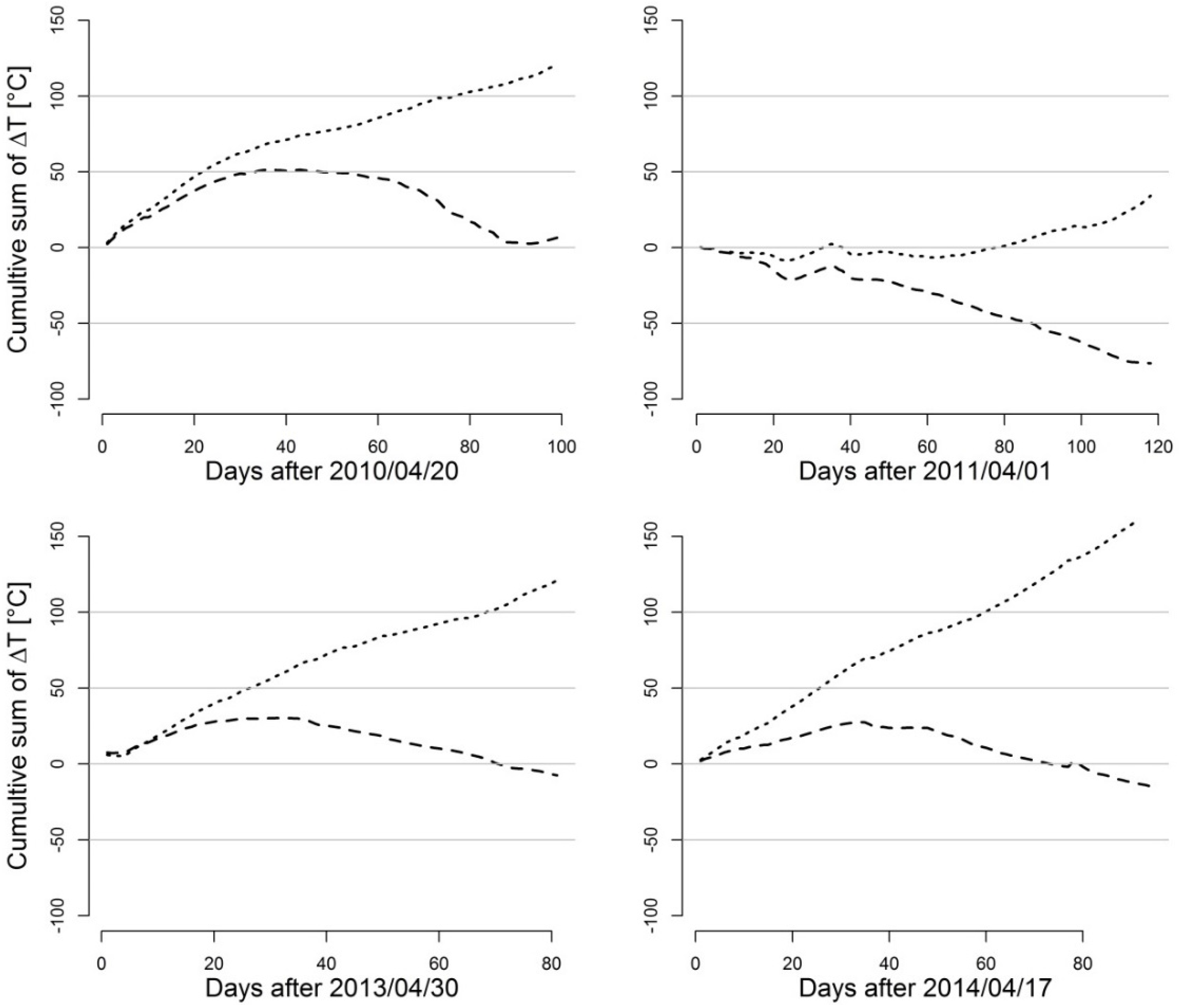
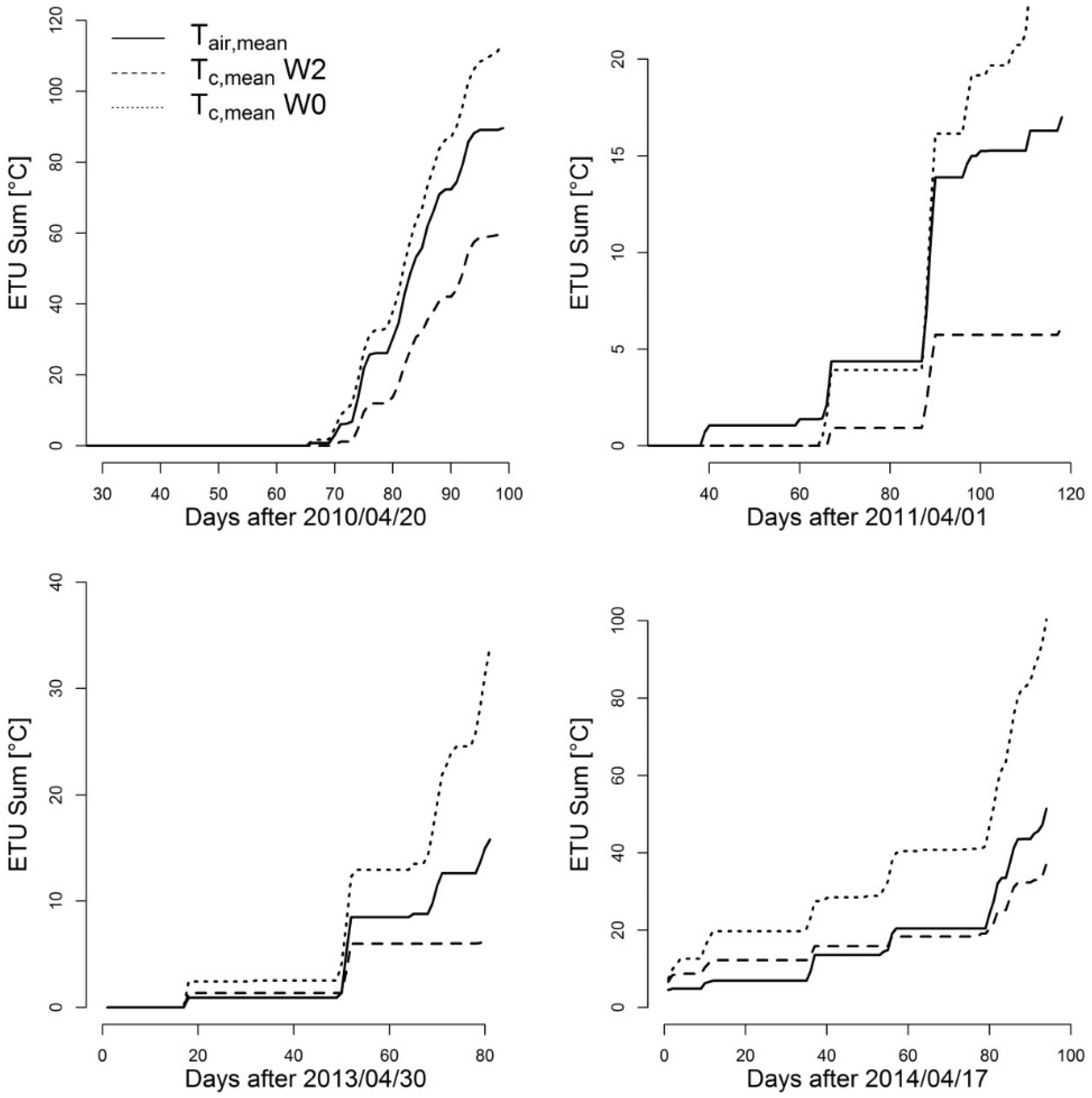
Statistical analyses and data processing were performed using R statistical software (http://www.R-project.org). The following packages were used: caret [45], FWDselect [46], Relaimpo [47], AED [48] and Quantreg [49].
Environmental and meteorological variables were selected to formulate simple regression models which are able to predict daily minimum, mean and maximum canopy temperatures (Tc,min, Tc,mean and Tc,max). Selected covariates are observed at standard meteorological stations (net radiation (Rn), total incoming radiation (Rint), air temperature (Tair), humidity (RH) and saturation vapor pressure deficit of the air (VPD), rainfall (R) and wind speed (W)) or commonly available from the output of crop system models (as specified in the following). Using the HUME model (cf. Section 2.3), we simulated time series data of crop height and leaf area index and calculated the main components of the plant-water-cycle, such as the total and plant available soil water content, ETA (= Eact + Tact), ETP, Tpot and Tact, Epot and Eact (cf. Section 2.3). We transformed absolute model results to relative values by formulating a range of ratios based on the available possible combinations of these variables, characterizing plant and soil water relations independent from the absolute amount of available water. Different formulations describing the evaporation (Eact/ETP and Eact/ETA, Eact/Epot) and the transpiration (Tact/ETP, Tact/ETA, Tact/Eact, Tact/Tpot) were applied as potential model covariates. Furthermore, we tested the suitability of the interpolated LAI, the natural logarithm of the LAI (LAIlog) and crop height (CH) values as predicting variable and tested for potential interaction effects between modeled environmental (as specified above) and meteorological data.
By using a random sampling strategy (CreateDataPartition function [45]) the whole data set (685 observation days, cf. Table 1) was partitioned in a training (50%) and a testing data subset (50%). Optimized combinations of covariates for a multiple linear regression model (maximum R2) were automatically calculated using a forward stepwise-based selection procedure (FWDselect function [46]). Meteorological, as well as environmental data are generally strongly inter-correlated. We assessed the multicollinearity of the co-variables by using the variance inflation factors (VIF; corvif function [48]) and consider VIF ≤3 as a benchmark [50]. Model reformulation and optimization were based on a quantile regression (QR) analysis (qr function [49]). The quantile regression is based on the conditional quantiles of the response variable distributions, thus, offering a more complete view of possible causal relationships between variables and useful for ecological applications with a limited number of available and strongly interacting variables [51]. Results from the quantile regression showed that the contributions of the selected independent variables to the conditional distribution of the canopy temperatures can vary significantly at different levels of canopy temperatures. Such patterns are hidden in ordinary multiple least-square regression model analyses. The predictive quality of the explanatory variables when applied to the training and testing data was identified at the 5% level of significance (p < 0.05).

2.5. Impact Study

To highlight the impact of using canopy instead of air temperatures in crop system models we performed an impact study for the observation years 2010 (20 April–27 July), 2011 (1 April–27 July), 2013 (30 April–19 July) and 2014 (17 April–19 July). Tc,mean, Tc,min and Tc,max for a well-irrigated wheat plot (W2) and for a not irrigated wheat plot (W0) are computed using the multiple linear regression models presented in this study (cf. Section 2.4) using data from the HS research site (cf. Section 2.1). Most crop system models apply air temperature-based “heat units” and use temperature thresholds to simulate the impact of temperatures on crop development, crop physiological processes and crop yield. To highlight the potential impact of the differences between air and crop temperatures on corresponding model results, we
(I)
calculate cumulative sum curves of the difference between modeled daily canopy temperature and the air temperature (∆T),
(II)
compute the number of days where modeled and measured canopy temperatures and air temperatures exceed temperature thresholds of 20 °C, 25 °C and 30 °C,
(III)
calculate extreme thermal unit (ETU) sums above the optimal temperature of 20 °C (according to [52]).
ETUs are calculated as the cumulative sums of the difference between the actual crop or air temperature, respectively, and the optimum temperature of 20 °C, where ETU = 0 if the actual temperature is below the optimum temperature [52].

3. Results and Discussion

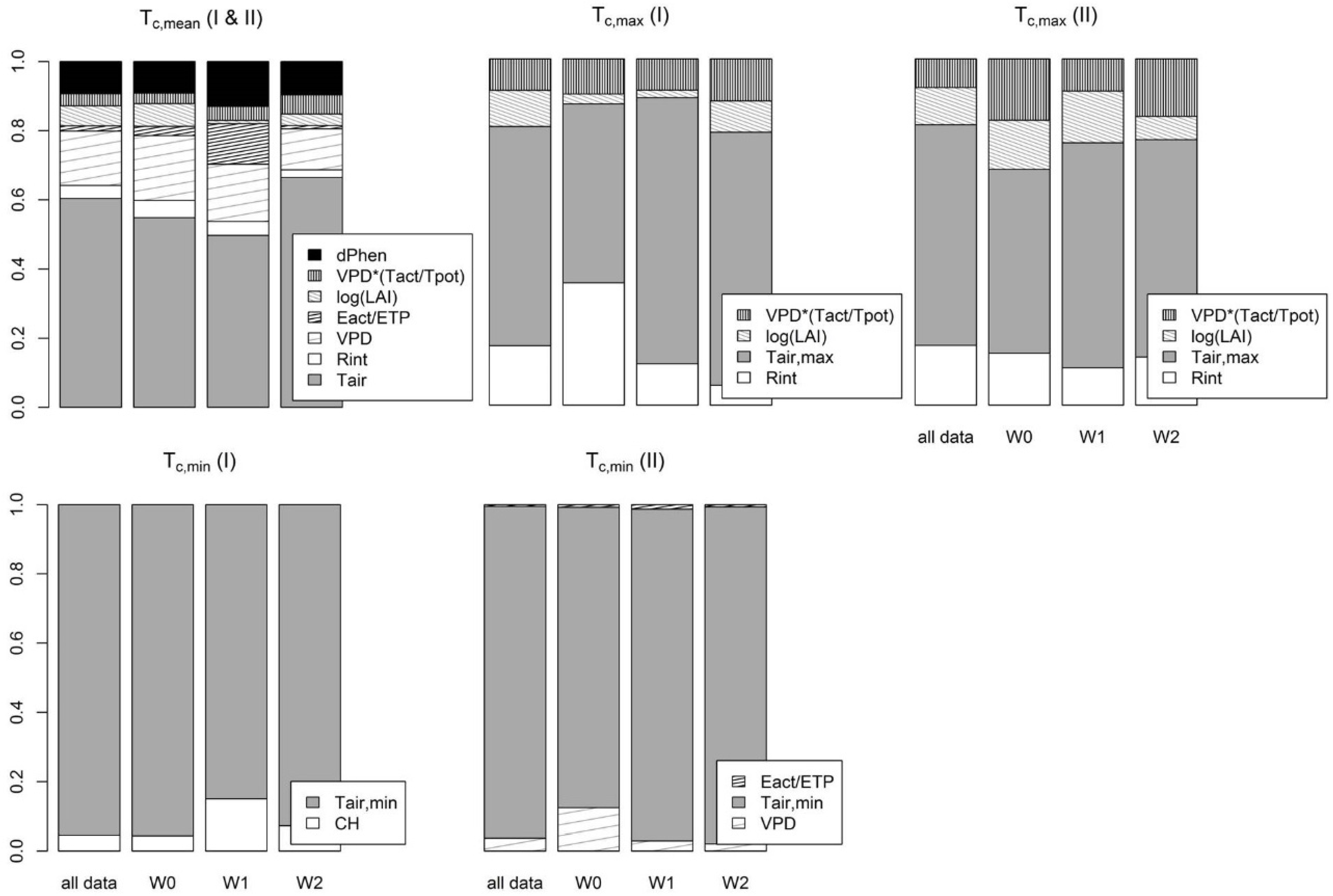
3.1. Empirical Models of Daily Canopy Temperatures

In the following, we provide a brief description of the multiple linear regression models developed for estimating Tc,mean, Tc,min and Tc,max (cf. Section 2.4) as a major result from our study. The relative importance of the covariates for the total estimated R2 is described and discussed in Section 3.3.
Based on the results from the quantile regression analyses (data not shown) empirical canopy temperature models were fitted to observations during the pre-heading (corresponding to stages <50 of the Zadoks scale) and during the post-heading (>50 of the Zadoks scale) phase. During the pre-heading phase (phase I), the conditional quantile contribution of environmental and meteorological factors to the canopy temperature significantly varied from their contribution during the post-heading phase (phase II), leading to significant changes in estimated model coefficients (models of Tc,min and Tc,max) and/or selection of model covariates (models of Tc,min and Tc,mean).
For simulating the daily mean canopy temperature (Tc,mean), the covariates explaining more than 90% of the total variability are the mean daily air temperature (°C), the incoming radiation (Rint (W·m−2)), the natural logarithm of the leaf area index (LAIlog), the vapor pressure deficit (VPD (hPa), only for phase I), the ratio of actual evaporation to ETP (Eact/ETP, only for phase II) and the product of the transpiration ratio, defined as the ratio of actual transpiration to the potential transpiration, and the VPD ((VPD*(Tact/Tpot)), only for phase II). We account for the changing contribution of the VPD, the Eact/ETP ratio and the product of transpiration ratio and VPD by using a dummy variable (DPhen), which equals 1 in the pre-heading and 0 in the post-heading phase (Table 2).
Table 2. Statistics of the multiple linear regression model developed using a forward stepwise-based selection procedure and quantile regression analyses for predicting Tc,mean (Tc,mean = mean daily canopy temperature) of a winter wheat canopy; SE = standard error, Tair,mean = mean daily air temperature (°C), Rint = incoming radiation (Wm−2), LAIlog = natural logarithm of the leaf area index, Dphen = phenology dummy variable with Dphen = 1 during phase I (pre-heading) and Dphen = 0 during phase II (post-heading, cf. Section 3.1), VPD = vapor pressure deficit (hPa), Tact/Tpot = transpiration ratio (Tact = actual and Tpot = potential transpiration (both in mm·d−1)), Eact/ETP = ratio of actual evaporation (Eact (mm·d−1)) to potential evapotranspiration (ETP (mm·d−1)).
EstimateSEp-Value
I & III & III & II
Intercept2.7300.266<2e−16
Tair,mean0.9420.015<2e−16
Rint0.0050.0011.27e−13
LAIlog−1.3580.082<2e−16
(1-Dphen)*Eact/ETP−5.4910.9531.87e−08
Dphen*VPD−0.2630.023<2e−16
(1-Dphen)*(VPD*(Tact/Tpot))−0.2990.033<2e−16
Tc,max are modeled using Rint, Tair,max, the natural logarithm of the leaf area index and the product of transpiration ratio and VPD. For the pre- and the post-heading phase significant changes in the model coefficients were calculated, thus, two model equations were derived (Table 3). For the pre-heading phase, Tc,min can be approximated using Tair,min and the canopy height (CH (m)). For the post-heading phase, it is simulated using the minimum diurnal air temperature, the VPD and the ratio of actual evaporation to ETP (Table 4).
Table 3. Statistics of the multiple linear regression model developed using a forward stepwise-based selection procedure and quantile regression analyses for predicting Tc,max (= maximum daily canopy temperature) of a winter wheat canopy; SE = standard error, Tair,max = maximum daily air temperature (°C), Rint = incoming radiation (Wm−2), LAIlog = natural logarithm of the leaf area index, VPD = vapor pressure deficit (hPa), Tact/Tpot = transpiration ratio (Tact = actual and Tpot = potential transpiration (both in mm·d−1)).
EstimateSEp-Value
IIIIIIIII
Intercept4.2414.0110.9420.6331.39e−051.58e−09
Rint0.0160.0140.0020.0021.75e−091.15e−15
Tair,max0.9220.8880.0550.029<2e−16<2e−16
LAIlog−2.816−1.8470.3400.1768.59e−14<2e−16
VPD*(Tact/Tpot)−0.447−0.6230.1130.0630.000118<2e−16
Table 4. Statistics of the multiple linear regression model developed using a forward stepwise-based selection procedure and quantile regression analyses for predicting Tc,min (= minimum daily canopy temperature) of a winter wheat canopy; SE = standard error, Tair,min = minimum daily air temperature (°C), CH = crop height (m), VPD = vapor pressure deficit (hPa), Eact/ETP = ratio of actual evaporation (Eact (mm·d−1)) to potential evapotranspiration (ETP (mm·d−1)).
EstimateSEp-Value
IIIIIIIII
Intercept1.116−0.2020.4100.2760.007290.466
CH−4.147-0.546-3.64e−12-
VPD-−0.101-0.019-2.89e−07
Tair,min1.0881.0130.0310.024<2e−16<2e−16
Eact/ETP-−3.158-0.715-1.65e−05

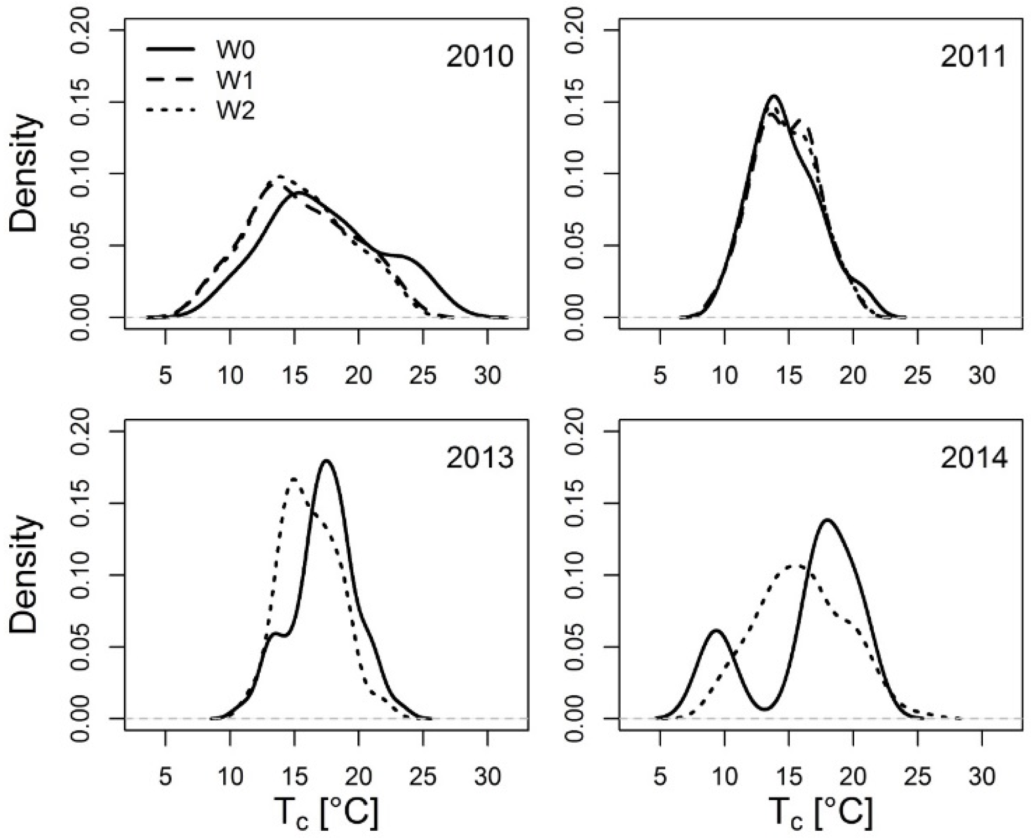
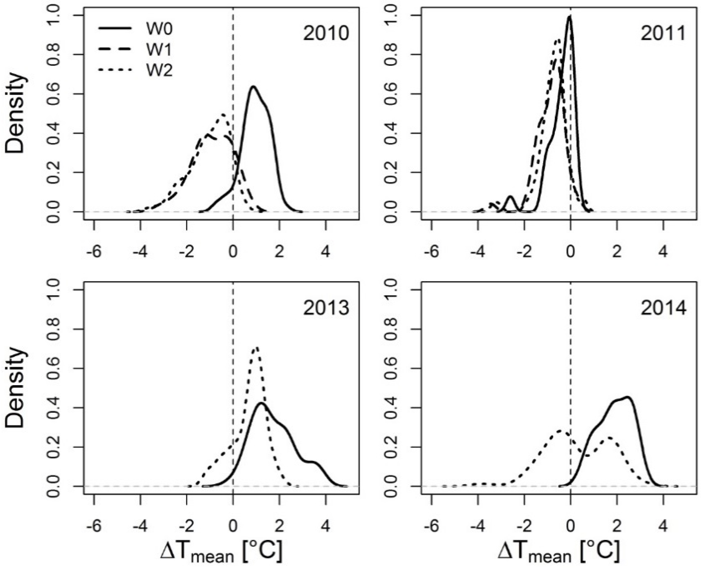
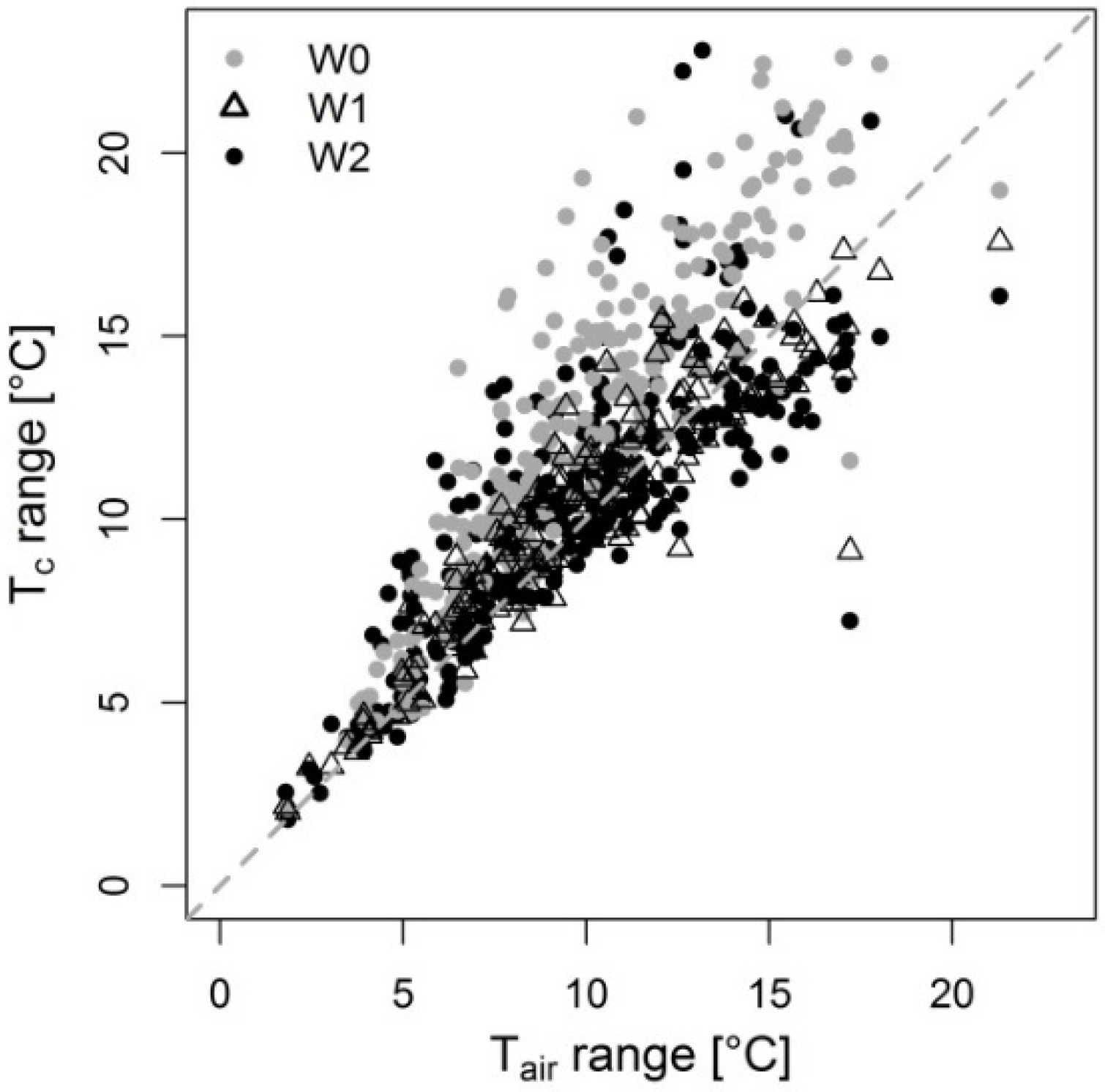
3.2. Variability of Canopy Surface Temperatures

In general, canopy temperatures of the drought treatment plots (W0) exceeded air temperatures (Figure 2), while the W1 and the W2 treatment canopy temperatures are lower (W1) and scatter more strongly (W2). Increased canopy temperatures result from the combined effect of decreased transpiration and evaporation levels of the plants and the underlying soil, respectively (cf. Section 3.3 for a discussion). The scattering of the W2 treatment data set can be mainly attributed the larger number of observations compared to the W1 and W0 treatments (cf. Table 1). Daily averaged surface temperatures (Tc,mean) range from ~8 °C to 26.5 °C (Figure 1) and daily averaged differences between canopy and air temperatures from −4 °C to +3.8 °C (ΔTmean) (Figure 3).
Figure 2. Scatter plot of mean, maximum and minimum canopy temperatures (Tc) and mean, maximum and minimum air temperatures (Tair) derived from the aggregation of hourly measurement data to daily values for three different irrigation treatments (W0 = no irrigation, W1 = medium deficit irrigation and W2 = full irrigation, r = Pearson’s correlation coefficient). The dashed black line indicates the line of identity.
Agronomy 06 00007 g002
Figure 3. Density plot of the mean daily difference between crop and air temperatures (∆Tmean) for the different observation years and irrigation treatments (W0 = no irrigation, W1 = medium deficit irrigation and W2 = full irrigation).
Agronomy 06 00007 g003
Compared with those of the irrigated plots, mean daily temperature differences between canopy and air (∆Tmean) values of the W0 treatment are clearly shifted towards higher values (Figure 3), indicating decreased stomatal aperture and lower transpiration levels under drought stress. The diurnal range of canopy temperatures measured at W0 plots clearly exceeds the diurnal range of air temperatures (Figure 4).
Figure 4. Scatter plot of the daily range of canopy temperatures (Tc, hourly values) and air temperatures (Tair, hourly values) for the complete observation period and for all irrigation treatments (W0 = no irrigation, W1 = medium deficit irrigation and W2 = full irrigation).
Agronomy 06 00007 g004

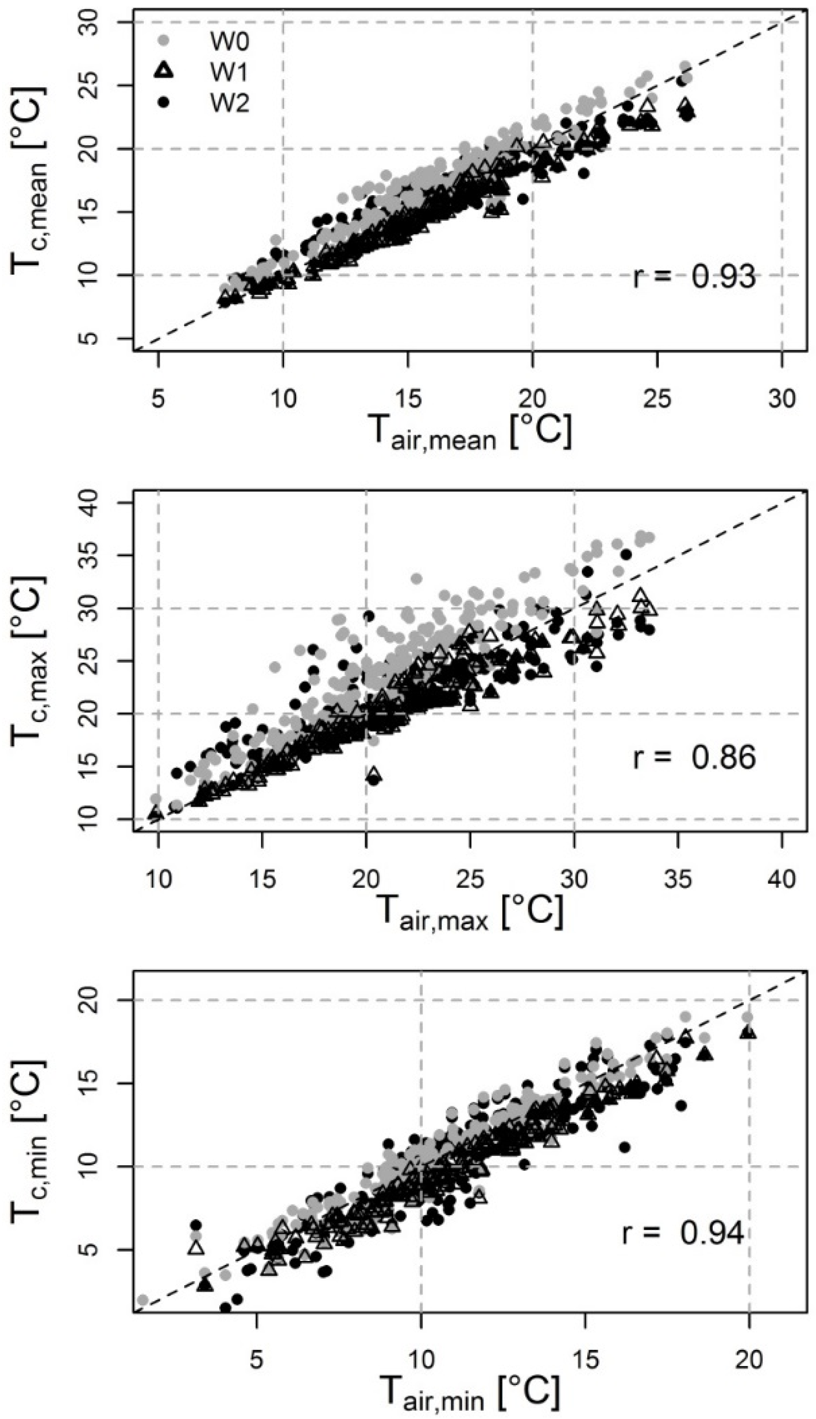
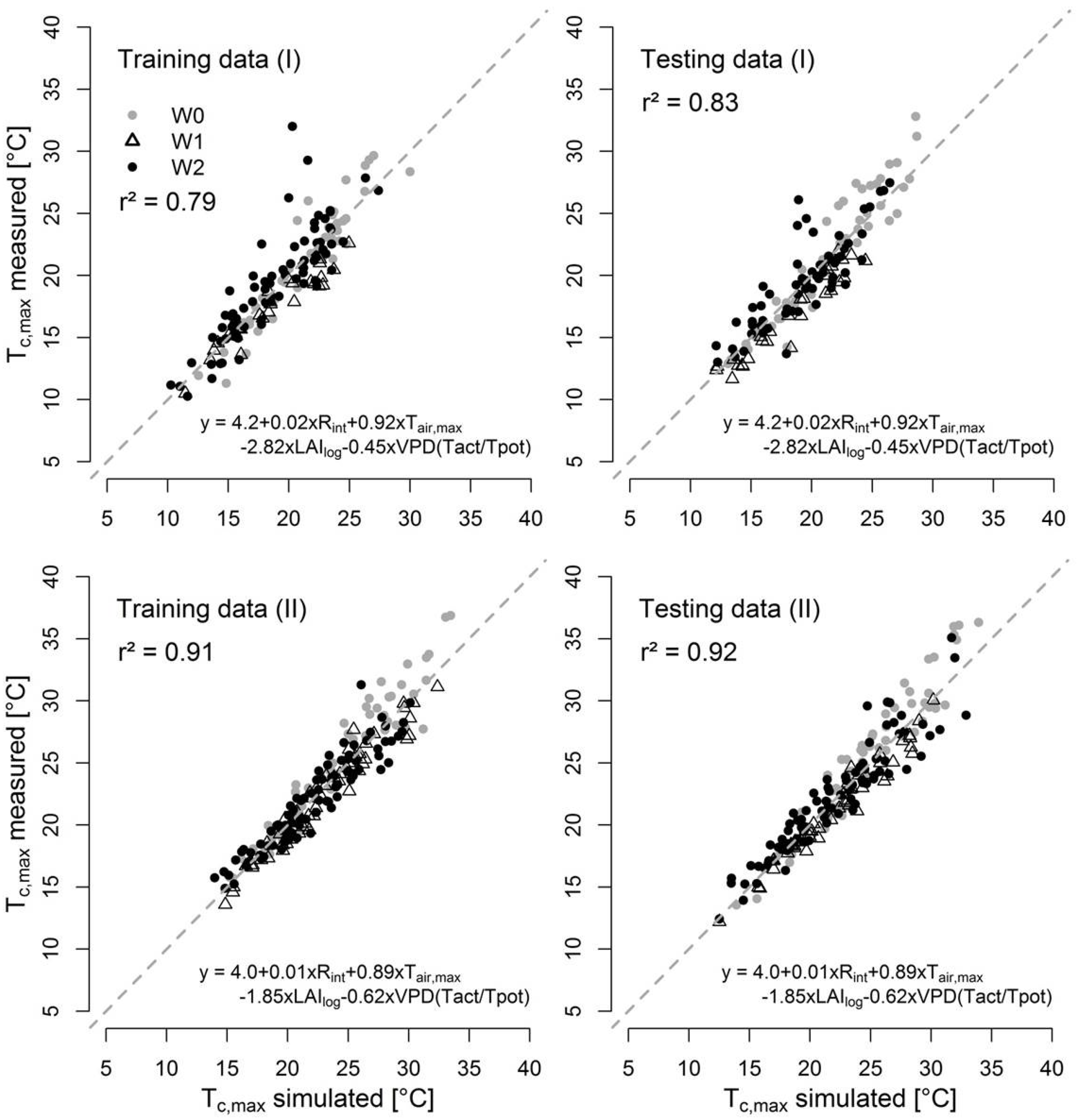
3.3. Predictive Ability of the Empirical Canopy Temperature Models

The standard cross validation revealed a root mean square error (RMSE) of ~0.8 °C for estimating Tc,mean, 2 °C (Phase I) and 1.5 °C (Phase II) for estimating Tc,max and 1.2 °C (Phase I) and 0.8 °C (Phase II) for estimating Tc,min, and could generalize well to the training data set (Table 5).
While the multiple linear regression model suggests a positive effect of radiation and air temperature, Tc,mean decreases with increasing LAI (Table 2). We calculated a negative slope for the VPD during the pre-heading phase and for the Eact/ETP ratio and the VPD-scaled transpiration ratio during the post-heading phase. The negative effect of the LAI and the VPD can be related to an increased transpiration cooling with increasing evaporative demand of the air and an increasing amount of transpiring plant tissues during the pre-heading stages. After the canopy has reached maximum leaf area and maximum height, during the post-heading stage, environmental conditions are characterized by decreased availability of soil water and increased air temperatures. Thus, for subsequent developmental stages, daily transpiration and evaporation help explain the variability of Tc,mean. An increasing fraction of actual evaporation (Eact) from the soil, e.g., after rain events, decreases the amount of energy available for heating the canopy (sensible heat fluxes). The increased latent heat flux arising from the soil further lowers the near-surface temperature. The negative slope of the VPD-scaled transpiration ratio can be related to the cooling effect of a higher amount of plant available soil water, weighted over the root distribution parameters and scaled with the evaporative demand of the air, on canopy temperatures.
The day-to-day variability of the maximum daily canopy temperatures can be simulated using incoming radiation, maximum daily air temperatures, the LAI and the VPD-weighed transpiration ratio (Table 3). Model coefficients differ for pre- and post-heading stages. The RMSE is higher for canopy temperatures simulated for the pre-heading stage (Table 5). The most likely cause is the higher overall range and day-to day variability of meteorological data typical for spring season conditions.
Table 5. Results of the multiple linear regression fit for all data and for the different irrigation treatments (W0–W2, cf. Section 2.1) using phenological subsets (I = pre-heading phase, II = post-heading phase) for modeling Tc,mean (mean daily canopy temperature (°C)), Tc,max (maximum daily canopy temperature) and Tc,min (minimum daily canopy temperature). R2 and the root mean squared error (RMSE (°C)) are given for the training (50% of all observations) and the testing data (50% of all observations).
Target VariableTreatmentPhaseTrainingTesting
R2RMSER2RMSE
Tc,meanAllI & II0.950.780.940.81
W0I & II0.970.640.950.72
W1I & II0.990.360.990.39
W2I & II0.920.880.930.87
Tc,maxAllI0.792.080.831.84
W0I0.891.620.911.60
W1I0.910.860.930.94
W2I0.742.290.721.90
Tc,maxAllII0.911.430.91.56
W0II0.931.480.921.49
W1II0.950.970.960.77
W2II0.891.260.881.52
Tc,minAllI0.91.040.861.19
W0I0.91.020.891.04
W1I0.920.730.751.00
W2I0.91.110.881.29
Tc,minAllII0.910.810.910.85
W0II0.940.670.930.80
W1II0.970.450.960.54
W2II0.890.890.880.95
During the early vegetative phase, additional influences of soil temperatures and soil optical properties on radiometric temperatures, in particular at low LAI levels as observed in the drought treatment plots, cannot be ruled out. Short-term influences, such as the effect of rapid fluctuations of wind and radiation on maximum daily canopy temperatures which cannot be incorporated in the model if operated at a daily resolution are probably responsible for the underestimation of temperatures >30 °C (Figure 5). However, the RMSE is <2 °C, thus, simulated temperatures are clearly closer to the measured canopy temperatures than air temperatures, especially for the W0 treatment (Figure 2). Note that the number of observation days where air temperatures exceed 30 °C is limited.
Minimum daily canopy temperatures, mostly representing night or early morning temperatures (data not shown), are simulated well (RMSE ~1 °C) using minimum air temperatures and by using crop height (for phase I), or VPD and the Eact/ETP ratio (for phase II) as additional explanatory variables (Table 4). During plant growth (phase I), the crop height is a controlling factor of the night-time temperature profiles, and, consequently, affects the radiometric temperatures measured by the infrared thermometers. As found for Tc,mean, for subsequent developmental stages, components of the canopy water balance help explain the variability of Tc,min. At night, transpiration is low or close to zero, thus, the actual evaporation is a suitable model covariate. Night-time or early-morning evaporation is driven by the evaporative demand of the air (VPD), giving reason for using VPD as a model covariate.
Note, that daily mean, maximum and minimum air temperatures were derived from hourly diurnal temperature measurements. The accuracy of models using temperatures characterized by higher uncertainty needs to be investigated in future studies.
Figure 5. Scatter plot of the measured and the simulated maximum daily canopy temperatures (Tc,max) for the training and the testing data set during the pre-heading (I) and the post-heading phase (II) for all irrigation treatments (W0 = no irrigation, W1 = medium deficit irrigation and W2 = full irrigation). The dashed gray line shows the line of identity. Equations of the multiple linear regression models and r2 (= coefficient of determination) are given (abbreviations as for Table 2, Table 3 and Table 4).
Agronomy 06 00007 g005
Calculations of the relative importance of the covariates for the total estimated R2 of the presented empirical models (Figure 6) highlight the dependence of their contribution on the crop water status: while, for the fully irrigated plots (W2), the air temperature contributes from ~60%–70% up to nearly 100% to the estimated R2 of the multiple linear regression (MLR) model, the contribution decreases to <50% for Tc,mean and Tc,max of the W0 plots. In consequence, the percentage contribution of, e.g., incoming radiation and the VPD to the R2 of the W0 canopy temperature models increases. Consequently, for simulating canopy temperatures under the influence of water deficits, solemnly using air temperature does not provide a suitable proxy for temperatures at the canopy level, and interactions between environmental and meteorological variables need to be incorporated.
A widely applied strategy to model temperature conditions within a crop canopy is the use of surface energy balance models [22,23]. Since such models are optimized to simulate the partitioning of available energy in latent and sensible heat fluxes, derived canopy temperatures are unrealistic if underlying assumptions, such as the closure of the energy balance, are not fulfilled. They are computationally expensive and require data on land surface physical parameters and aerodynamic properties of the canopy. Anomalies of these variables with respect to “average conditions”, which are common for water-limited conditions, limit the use of standard literature values. Consequently, the use of derived canopy temperatures in crop system models is limited. Contrastingly, suggested empirical models are a strong simplification of the complex processes related to the crop canopy temperature dynamics [2,4,17] and do not predict canopy temperatures over different scales in time and space. However, the aim of our study was to provide a practical tool in plant growth models for reliable canopy temperature predictions using a small number of input variables. Presented models were designed for simulating the winter wheat canopy temperature during stem extension, heading and ripening growth stages. For transferring them to other crops and/or observation scales, equations can be refitted using local radiometric temperature observations, micrometeorological measurements and the output of a day step model. Coupling such empirical models to existing crop system models allows for including realistic near surface and canopy temperatures for site- and scale-specific estimates of crop development and the impact of heat stress on crop yield, provided that these models reliably simulate the components of the soil water balance. We are aware that current agroecosystem models were designed to use air temperatures as input for simulating plant development and the impact of heat stress. This may imply the need for the recalibration of some parameters of temperature-dependent processes. However, the simulation of canopy temperatures is an important step towards a more realistic representation of temperature stress effects and the interaction between heat and drought stress in models [15], thus, for simulating the effect of temperatures as a limiting, defining and reducing factor.
Figure 6. Estimated relative importance of covariates for simulating Tc,mean, Tc,max and Tc,min for the training data set during the pre-heading (I) and the post-heading phase (II). Abbreviations as for Table 2, Table 3 and Table 4.
Agronomy 06 00007 g006

3.4. Case Study: Wheat Canopy versus Air Temperature

The shape of the cumulative sum curves of the difference between daily averaged canopy temperature and the air temperature (∆T) is highly dependent on the observation year (Figure 7). However, cumulative ∆T sums of the drought treatment plot (W0) almost constantly increase throughout the growing season, i.e., in 2014 (Figure 7). Contrastingly, we calculated negative cumulative sums of ∆T for the well irrigated plot (W2) at the end of the growing season (except in 2010). In 2011 and 2013, the canopy of the irrigated plot is almost constantly cooler compared to the air temperature, whereas, in 2010 and 2014, it was warmer until mid/end of June and cooler during the subsequent growing stages. Our data indicate increasing negative temperature anomalies for fully irrigated and positive anomalies for not irrigated wheat plots during the period ranging from the flowering stage until maturity. Obviously, during these periods, the higher level of canopy transpiration of fully irrigated crops can significantly reduce the effect of short-term heat events on plant physiological processes. Although modeled and measured absolute canopy temperatures from our study might strongly differ from those data observed at other crops, sites, and observation years, we assume that such differences between air and canopy temperatures of irrigated and non-irrigated plots are critical for the results of crop system models.
Figure 7. Cumulative sums of canopy to air temperature differences (∆T (°C)) for the drought treatment plot (dotted line) and the irrigated plot (dashed line) using mean daily modeled surface temperatures (∆T = Tc,mean–Tair,mean) in 2010 (top left), 2011 (top right), 2013 (bottom left), 2014 (bottom right) (Hohenschulen research site).
Agronomy 06 00007 g007
If using maximum air temperatures (Tair,max), the number of days exceeding temperature thresholds of 20 °C and 25 °C is close to that of using maximum canopy temperatures from the fully irrigated treatment plot (Table 6). However, the number of days is significantly higher if using Tc,max W0. Note that measured temperatures for the drought treatment plot from 2014 are only available until beginning of May and that there is a data gap of seven days in 2011 (Table 1). Despite large interannual differences in the number of days exceeding sample temperature thresholds, our data highlight the need to account for air-canopy temperature differences in threshold-based modeling approaches.
To highlight the impact of temperature differences on summed thermal units, which are frequently used in models to simulate crop development, we computed ETU sums above the optimal temperature of 20 °C [52]. Patterns of the sum curves clearly indicate lowest values if using Tc,mean W2 and highest values using Tc,mean W0 (Figure 8). Note that starting dates differ for each observation year. Absolute summed differences increase during the wheat flowering and ripening stages. It is well known that the difference between canopy and air temperatures increases at higher levels of crop water stress. Our results, however, suggest significant discrepancies in Tair,mean- and Tc,mean-based ETU calculations not only for the drought treatment but also for the well irrigated plot. These differences can be critical for the simulation of the timing of crop developmental stages.
Table 6. Number of days exceeding 20, 25 and 30 °C for modeled maximum daily crop temperature of the drought treatment plot (Tc,max W0) and the irrigated plot (Tc,max W2) and for the measured maximum daily air temperature (Tair,max) in 2010, 2011, 2013 and 2014 (Hohenschulen research site). In parentheses, values calculated for available measured canopy temperatures are given (cf. Table 1).
VariableYearDays > 20 °CDays > 25 °CDays > 30 °C
Tc,max W0201060 (61)30 (36)12 (17)
Tc,max W2201055 (42)20 (14)2 (0)
Tair,max201053 (55)19 (20)10 (10)
Tc,max W0201155 (26)12 (8)1 (0)
Tc,max W2201144 (30)4(6)0 (0)
Tair,max201142 (34)7 (6)0 (0)
Tc,max W0201355 (47)29 (33)3 (7)
Tc,max W2201337 (34)6 (5)0 (0)
Tair,max201331 (29)9 (9)1 (1)
Tc,max W0201477 (13)36 (5)12 (0)
Tc,max W2201459 (68)15 (26)1 (3)
Tair,max201454 (53)13 (18)0 (3)
Figure 8. Extreme thermal unit sums above the optimal temperature of 20 °C (ETU, [52]) for the modeled mean daily crop temperature of the drought treatment plot (Tc,mean W0, dotted line), the fully irrigated plot (Tc,mean W2, dashed line) and for the measured mean daily air temperature (Tair,mean, solid line) in 2010 (top left), 2011 (top right), 2013 (bottom left), 2014 (bottom right) (Hohenschulen research site).
Agronomy 06 00007 g008
Crops show threshold responses to meteorological and environmental conditions, especially to temperature [53,54]. Current crop system models use the sum of daily temperatures exceeding a base temperature and crop-specific temperature thresholds (cardinal temperatures) for deriving factors and/or linear and non-linear response functions controlling the simulation of phenology, growth (biomass accumulation), biochemical processes (nutrient uptake) and the harvest index. Well defined threshold responses are generally derived from growth chamber experiments performed under controlled conditions. We suggest avoiding the use of air temperatures recorded at 1.5 or 2 m height above the canopy for threshold-based modeling approaches since large positive or negative temperature anomalies to the near-surface temperatures can be expected. Such differences can have important consequences for the accuracy of plant physiological processes and crop yield simulations.
Currently, few models are able to account for increasing canopy temperatures during drought stress by offering optional corrective temperature mechanisms based on water stress indices [12,55]. However, next to the effects of drought stress on canopy temperatures our study further highlights the importance of considering negative temperature anomalies (transpiration cooling) found for fully irrigated crops, when simulating crop phenological development and the impact of heat stress effects on crop yields.

4. Conclusions

Canopy temperatures of water-deficit and fully irrigated wheat plots significantly differ from air temperature measurements. Such temperature anomalies need to be considered in crop system models. Variables available from daily standard meteorological observations (vapor pressure deficit, minimum, maximum and mean temperature, incoming radiation) and from widely applied agro-ecosystem models (potential and actual transpiration, evaporation, leaf area index, and crop height) allow for approximating wheat canopy temperatures using simple empirical linear regression models. Significant differences in model coefficients for the pre- and the post-heading phase can be related to the stronger influence of the components of the crop and the soil water balance during the post-heading stage. The use of canopy temperatures as an input for crop system models will lead to the need for adapting temperature thresholds and the temperature sum calculations. However, canopy temperatures provide a more realistic measure of microclimatic conditions and their potentially amplifying or mitigating effect on plant response to temperature stress.

Acknowledgments

This work was funded by German Research Foundation (DFG). We would like to thank Doris Ziermann for her expert technical assistance with the field measurements.

Author Contributions

Dorothee Neukam is responsible for the realization of the study, and significantly contributed to the interpretation and the analysis of the results. Hella Ahrends is responsible for the preparation of the manuscript, the analysis and the interpretation of the results. Adam Luig significantly contributed to the design of the study, to the data analyzed within this study and the interpretation of the results. Remy Manderscheid and Henning Kage significantly contributed to the realization of the study, data availability and to the interpretation of the results.

Conflicts of Interest

The authors declare no conflict of interest.

References

  1. Hoogenboom, G. Contribution of agrometeorology to the simulation of crop production and its applications. Agric. For. Meteorol. 2000, 103, 137–157. [Google Scholar] [CrossRef]
  2. Gates, D.M. Transpiration and Leaf Temperature. Ann. Rev. Plant Physiol. 1968, 19, 211–238. [Google Scholar] [CrossRef]
  3. Burke, J.J.; Upchurch, D.R. Leaf temperature and transpirational control in cotton. Environ. Exp. Bot. 1989, 29, 487–492. [Google Scholar] [CrossRef]
  4. Jones, H.G. Plants and Microclimate: A Quantitative Approach to Environmental Plant Physiology; Cambridge University Press: Cambridge, UK, 2013. [Google Scholar]
  5. Rezaei, E.; Webber, H.; Gaiser, T.; Naab, J.; Ewert, F. Heat stress in cereals: Mechanisms and modelling. Eur. J. Agron. 2015, 64, 98–113. [Google Scholar] [CrossRef]
  6. Jarvis, P.P.G. Coupling of transpiration to the atmosphere in horticultural crops: The omega factor. Acta Hortic. 1985, 171, 187–206. [Google Scholar] [CrossRef]
  7. Tanny, J. Microclimate and evapotranspiration of crops covered by agricultural screens: A review. Biosyst. Eng. 2013, 114, 26–43. [Google Scholar] [CrossRef]
  8. Van Oort, P.A.J.; Saito, K.; Zwart, S.J.; Shrestha, S. A simple model for simulating heat induced sterility in rice as a function of flowering time and transpirational cooling. Field Crops Res. 2014, 156, 303–312. [Google Scholar] [CrossRef]
  9. Alderman, P.; Quilligan, E.; Asseng, S.; Ewert, F.; Reynolds, M. Proceedings of the Workshop on Modeling Wheat Response to High Temperature, Texcoco, Mexico, 19–21 June 2013; CIMMYT: El Batán, Mexico, 2013. [Google Scholar]
  10. Cho, J.; Oki, T. Application of temperature, water stress, CO2 in rice growth models. Rice 2012, 5. [Google Scholar] [CrossRef]
  11. Siebert, S.; Ewert, F.; Rezaei, E.E.; Kage, H.; Graß, R. Impact of heat stress on crop yield—On the importance of considering canopy temperature. Environ. Res. Lett. 2014, 9. [Google Scholar] [CrossRef]
  12. Webber, H.; Martre, P.; Asseng, S.; Kimball, B.; White, J.; Ottman, M.; Wall, G.W.; de Sanctis, G.; Doltra, J.; Grant, R.; et al. Canopy temperature for simulation of heat stress in irrigated wheat in a semi-arid environment: A multi-model comparison. Field Crops Res. 2015. [Google Scholar] [CrossRef]
  13. Bassu, S.; Brisson, N.; Durand, J.L.; Boote, K.; Lizaso, J.; Jones, J.W.; Rosenzweig, C.; Ruane, A.C.; Adam, M.; Baron, C.; et al. How do various maize crop models vary in their responses to climate change factors? Glob. Chang. Biol. 2014, 20, 2301–2320. [Google Scholar] [CrossRef] [PubMed]
  14. Lamsal, A.; Amgai, L.; Giri, A. Modeling the sensitivity of CERES-Rice model: An experience of Nepal. Agron. J. Nepal 2013, 3, 11–22. [Google Scholar] [CrossRef]
  15. Levis, S. Crop heat stress in the context of Earth System modeling. Environ. Res. Lett. 2014, 9. [Google Scholar] [CrossRef]
  16. Jamieson, P.D.; Brooking, I.R.; Porter, J.R.; Wilson, D.R. Prediction of leaf appearance in wheat: A question of temperature. Field Crops Res. 1995, 41, 35–44. [Google Scholar] [CrossRef]
  17. Maes, W.H.; Steppe, K. Estimating evapotranspiration and drought stress with ground-based thermal remote sensing in agriculture: A review. J. Exp. Bot. 2012, 63, 4671–4712. [Google Scholar] [CrossRef] [PubMed]
  18. Amani, I.; Fischer, R.A.; Reynolds, M.P. Canopy temperature depression association with yield of irrigated spring wheat cultivars in a hot climate. J. Agron. Crop Sci. 1996, 176, 119–129. [Google Scholar] [CrossRef]
  19. Ayeneh, A.; van Ginkel, M.; Reynolds, M.P.; Ammar, K. Comparison of leaf, spike, peduncle and canopy temperature depression in wheat under heat stress. Field Crops Res. 2002, 79, 173–184. [Google Scholar] [CrossRef]
  20. Rebetzke, G.J.; Rattey, A.R.; Farquhar, G.D.; Richards, R.A.; Condon, A.G. Genomic regions for canopy temperature and their genetic association with stomatal conductance and grain yield in wheat. Funct. Plant Biol. 2012, 40, 14–33. [Google Scholar] [CrossRef]
  21. Gautam, A.; Prasad, S.V.S.; Jajoo, A.; Ambati, D. Canopy temperature as a selection parameter for grain yield and its components in durum wheat under terminal heat stress in late sown conditions. Agric. Res. 2015, 4, 238–244. [Google Scholar] [CrossRef]
  22. Fang, Q.X.; Ma, L.; Flerchinger, G.N.; Qi, Z.; Ahuja, L.R.; Xing, H.T.; Li, J.; Yu, Q. Modeling evapotranspiration and energy balance in a wheat–maize cropping system using the revised RZ-SHAW model. Agric. For. Meteorol. 2014, 194, 218–229. [Google Scholar] [CrossRef]
  23. Maruyama, A.; Kuwagata, T. Coupling land surface and crop growth models to estimate the effects of changes in the growing season on energy balance and water use of rice paddies. Agric. For. Meteorol. 2010, 150, 919–930. [Google Scholar] [CrossRef]
  24. Jackson, R.D.; Reginato, R.J.; Idso, S.B. Wheat canopy temperature: A practical tool for evaluating water requirements. Water Resour. Res. 1977, 13, 651–656. [Google Scholar]
  25. Idso, S.B.; Jackson, R.D.; Pinter, P.J.; Reginato, R.J.; Hatfield, J.L. Normalizing the stress-degree-day parameter for environmental variability. Agric. Meteorol. 1981, 24, 45–55. [Google Scholar] [CrossRef]
  26. Yuan, G.; Luo, Y.; Sun, X.; Tang, D. Evaluation of a crop water stress index for detecting water stress in winter wheat in the North China Plain. Agric. Water Manag. 2004, 64, 29–40. [Google Scholar] [CrossRef]
  27. Bellvert, J.; Zarco-Tejada, P.J.; Marsal, J.; Girona, J.; González-Dugo, V.; Fereres, E. Vineyard irrigation scheduling based on airborne thermal imagery and water potential thresholds. Aust. J. Grape Wine Res. 2015. [Google Scholar] [CrossRef]
  28. Cohen, Y.; Alchanatis, V.; Sela, E.; Saranga, Y.; Cohen, S.; Meron, M.; Bosak, A.; Tsipris, J.; Ostrovsky, V.; Orolov, V.; et al. Crop water status estimation using thermography: Multi-year model development using ground-based thermal images. Precis. Agric. 2015, 16, 311–329. [Google Scholar] [CrossRef]
  29. Sieling, K.; Kage, H. N balance as an indicator of N leaching in an oilseed rape—Winter wheat—Winter barley rotation. Agric. Ecosyst. Environ. 2006, 115, 261–269. [Google Scholar] [CrossRef]
  30. Neukam, D.; Böttcher, U.; Kage, H. Modelling wheat stomatal resistance in hourly time steps from micrometeorological variables and soil water status. J. Agron. Crop Sci. 2015. [Google Scholar] [CrossRef]
  31. Zadoks, J.C.; Chang, T.T.; Konzak, C.F. A decimal code for the growth stages of cereals. Weed Res. 1974, 14, 415–421. [Google Scholar] [CrossRef]
  32. Weigel, H.; Pacholski, A.; Burkart, S.; Helal, M.; Heinemeyer, O.; Kleikamp, B.; Manderscheid, R.; Frühauf, C.; Hendrey, G.; Lewin, K.; et al. Carbon turnover in a crop rotation under free air CO2 enrichment (FACE). Pedosphere 2005, 15, 728–738. [Google Scholar]
  33. Erbs, M.; Manderscheid, R.; Weigel, H.J. A combined rain shelter and free-air CO2 enrichment system to study climate change impacts on plants in the field. Methods Ecol. Evol. 2012, 3, 81–88. [Google Scholar] [CrossRef]
  34. Kage, H.S.; Stützel, H. HUME: An object oriented component library for generic modular modelling of dynamic systems. In Proceedings of the 1st Modelling Cropping System International Symposium, Lleida, Spain, 21–23 June 1999; pp. 299–300.
  35. Kage, H.; Kochler, M.; Stützel, H. Root growth and dry matter partitioning of cauliflower under drought stress conditions: Measurement and simulation. Eur. J. Agron. 2004, 20, 379–394. [Google Scholar] [CrossRef]
  36. Johnen, T.; Boettcher, U.; Kage, H. An analysis of factors determining spatial variable grain yield of winter wheat. Eur. J. Agron. 2014, 52, 297–306. [Google Scholar] [CrossRef]
  37. Li, K.Y.; Jong, R.D.; Boisvert, J.B. An exponential root-water-uptake model with water stress compensation. J. Hydrol. 2001, 252, 189–204. [Google Scholar] [CrossRef]
  38. Van Genuchten, M.T. Closed-form equation for predicting the hydraulic conductivity of unsaturated soils. Soil Sci. Soc. Am. J. 1980, 44, 892–898. [Google Scholar] [CrossRef]
  39. Wösten, J.H.M.; van Genuchten, M.T. Using texture and other soil properties to predict the unsaturated soil hydraulic functions. Soil Sci. Soc. Am. J. 1988, 52, 1762–1770. [Google Scholar] [CrossRef]
  40. Monteith, J.L. Evaporation and environment. Symp. Soc. Exp. Biol. 1965, 19, 205–234. [Google Scholar] [PubMed]
  41. Thom, A.; Oliver, H. Penmans Equation for estimating regional evaporation. Q. J. R. Meteorol. Soc. 1977, 103, 345–357. [Google Scholar] [CrossRef]
  42. Beese, F.; van der Ploeg, R.; Richter, W. Der Wasserhaushalt einer Löss-Parabraunerde unter Winterweizen und Brache. Z. Acker Pflanzenbau 1978, 146, 1–19. (In German) [Google Scholar]
  43. Feddes, R.A.; Kowalik, P.J.; Zaradny, H. Simulation of Field Water Use and Crop Yield; Pudoc, Centre for Agricultural Publishing and Documentation: Wageningen, The Netherlands, 1978. [Google Scholar]
  44. Ehlers, W.; Hamblin, A.P.; Tennant, D.; van der Ploeg, R.R. Root system parameters determining water uptake of field crops. Irrig. Sci. 1991, 12, 115–124. [Google Scholar] [CrossRef]
  45. Kuhn, M. Building predictive models in R using the caret package. J. Stat. Softw. 2008, 28, 1–26. [Google Scholar] [CrossRef]
  46. Sestelo, M.; Villanueva, N.M.; Roca-Pardiñas, J. FWD select: An R package for selecting variables in regression models. Discuss. Papers Stat. Oper. Res. 2013, 13. Available online: http://depc05.webs.uvigo.es/reports/13_02.pdf (accessed on 21 January 2016). [Google Scholar]
  47. Grömping, U. Relative importance for linear regression in R: The package relaimpo. J. Stat. Softw. 2006, 17. [Google Scholar] [CrossRef]
  48. Zuur, A.; Ieno, E.N.; Walker, N.; Saveliev, A.A.; Smith, G.M. Mixed Effects Models and Extensions in Ecology with R; Springer Science + Business Media: New York, NY, USA, 2009. [Google Scholar]
  49. Koenker, R.; Hallock, K.F. Quantile Regression. J. Econ. Perspect. 2001, 15, 143–156. [Google Scholar] [CrossRef]
  50. Zuur, A.F.; Ieno, E.N.; Elphick, C.S. A protocol for data exploration to avoid common statistical problems. Methods Ecol. Evol. 2010, 1, 3–14. [Google Scholar] [CrossRef]
  51. Cade, B.S.; Noon, B.R. A gentle introduction to quantile regression for ecologists. Front. Ecol. Environ. 2003, 1, 412–420. [Google Scholar] [CrossRef]
  52. Gobin, A. Impact of heat and drought stress on arable crop production in Belgium. Nat. Hazards Earth Syst. Sci. 2012, 12, 1911–1922. [Google Scholar] [CrossRef]
  53. Porter, J.R.; Gawith, M. Temperatures and the growth and development of wheat: A review. Eur. J. Agron. 1999, 10, 23–36. [Google Scholar] [CrossRef]
  54. Porter, J.R.; Semenov, M.A. Crop responses to climatic variation. Philos. Trans. R. Soc. B Biol. Sci. 2005, 360, 2021–2035. [Google Scholar] [CrossRef] [PubMed]
  55. Stöckle, C.O.; Nelson, R.L. Cropping Systems Simulation Model User’s Manual; Biological Systems Engineering Department, Washington State University: Pullman, WA, USA, 2013; Available online: https://nishat2013.files.wordpress.com/2013/11/cropping-system-manual-book.pdf (accessed on 21 October 2015).

