
Assessing the Effectiveness of Pruning in an Olive Orchard Using a Drone and a Multispectral Camera: A Three-Year Study


Department of Agricultural, Food and Forest Sciences, University of Palermo, 90128 Palermo, Italy
*
Author to whom correspondence should be addressed.
Agronomy 2024, 14(5), 1023; https://doi.org/10.3390/agronomy14051023
Submission received: 13 March 2024
/
Revised: 7 May 2024
/
Accepted: 9 May 2024
/
Published: 11 May 2024
(This article belongs to the Special Issue Effects of Agrotechnical Factors and Farming Systems on Soil Properties and Plant Productivity)
Abstract
:The uses of precision oliviculture have increased in recent years to improve the quality and quantity of extra virgin olive oil. In traditional and intensive systems, biennial pruning is often applied to balance and maintain plant vigour, aiming at reducing management costs. This study presents the results of a three-year experiment with the objective of quantifying the effects of biennial pruning on the vegetative vigour of olive trees, investigating the geometric and spectral characteristics of each canopy determined with multispectral images acquired by UAV. The experiment was carried out in an olive orchard located in western Sicily (Italy). Multispectral images were acquired using a UAV in automatic flight configuration at an altitude of 70 m a.g.l. The segmentation and classification of the images were performed using Object-Based Image Analysis (OBIA) based on the Digital Elevation Model (DEM) and orthomosaic to extract the canopy area, height, volume and NDVI for each plant. This study showed that the technology and image analysis processing used were able to estimate vigour parameters at different canopy densities, compared to field measurements (R2 = 0.97 and 0.96 for canopy area and volume, respectively). Furthermore, it was possible to determine the amount of removed biomass for each plant and vigour level. Biennial pruning decreased the number of plants initially classified as LV (low-vigour) and maintained a vegetative balance for MV (medium-vigour) and HV (high-vigour) plants, reducing the spatial variability in the field.
1. Introduction
Agricultural techniques applied to olive orchards aim at increasing production efficiency, minimising the use of inputs and increasing environmental sustainability [1,2]. Olive cultivation is mainly concentrated in Europe, within the Mediterranean region, particularly in countries such as Spain, Italy and Greece, which together account for 61% of the global cultivated area [3]. In these cultivation regions, there is significant soil and climatic diversity, resulting in different growing conditions [4,5]. This variability in plots of various sizes causes waste of the applied resources. Therefore, it is important to implement agronomic techniques based on variable distribution systems according to effective requirements. For this purpose, variability evaluation can be carried out continuously and/or periodically using different technologies and sensors. In precision oliviculture, some studies have shown that the variability observed in olive production was closely linked to soil variability, in particular to the concentration of organic matter, nitrogen and electrical conductivity [6,7]. Scientific research has focused on the study of biophysical [8,9] and spectral parameters [10,11] to achieve a better understanding of the physiological state, vegetative vigour and productivity of plants. The main biophysical canopy parameters currently observed include canopy height (CH), canopy area (CA), canopy volume (CV) and, in some cases, canopy perimeter and penetrability [8,12,13]. Spectral parameters, on the other hand, are based on the study of plant reflectance in specific regions of the electromagnetic spectrum using various methodologies, including the determination of vegetation indices (VIs) [14,15]. The most commonly used vegetation index in olive orchards is the Normalised Different Vegetation Index (NDVI) [16], because it provides a good indication of biomass, nutritional, productive and physiological conditions by exploiting crop reflectance in the red and near-infrared bands [17]. Unmanned Aerial Vehicles (UAVs) are remote platforms capable of housing sensors that can detect vegetative and spectral conditions. They are widely used in olive groves for their versatility in different orographic conditions and ability to provide high-resolution images over extensive areas.
Once variability has been detected within an olive orchard, variable-rate agronomic techniques can be applied; these include irrigation [18], fertilisation [19], pest and disease control [20] and pruning [21].
Pruning is essential for balancing vegetative and reproductive activity, resource allocation and modifying canopy architecture [22]. In traditional and intensive olive groves, pruning cannot be standardised and represents a major management cost [23]. Therefore, mapping a plot’s vigour conditions would make it possible to predict vegetative development based on plant vigour and the intensity of pruning applied.
Most drone surveys of olive trees aim to quantify the amount of biomass removed according to different pruning levels, irrigation regimes or varieties [21,24,25]. Jiménez-Brenes et al. (2017) [21] determined the projected canopy area, height and volume of trees after three different types of pruning, observing that trees subjected to more aggressive pruning showed greater vegetative development. Pruning management typically involves characterising tree architecture through manual measurements in order to estimate canopy volume using empirical equations [26,27]. The combined use of UAV images, 3D models and Object-Based Image Analysis (OBIA) provides new opportunities for monitoring and applying differentiated management of olive orchard pruning [12,28] in order to regularise growth activity.
This study presents the results of a three-year experiment with the objective of evaluating the potential of multispectral images acquired by UAV to determine the geometric characteristics and spectral behaviour of olive tree canopies in order to quantify the effects of biennial pruning on the vegetative vigour of the plants.
2. Materials and Methods
2.1. Study Area
The experimental area is located in Segesta (province of Trapani, Italy; Figure 1); according to the Koppen–Geiger classification, the climate is Mediterranean with summer heat [29].
The soil belongs to the sand–clay–silt grain size class, according to the United States Department of Agriculture (USDA) classification. The plot surface is 5860 m2, with flat orography. The 20-year-old olive orchard (cv. Cerasuola) is cultivated using an intensive system, with planting distances 5.0 × 5.5 m; the direction of the rows is NE–SW at an angle of 60° to the north. The experiment was carried out from 2021 to 2023. In this period, the olive grove was managed according to the ordinary practices of the area, including biennial pruning. In 2021 and 2022, the trees grew for two vegetative cycles. At the end of the second year, intensive pruning was carried out (December 2022, BBCH00 vegetative stasis) in order to assess its effect on changes in vigour, which was evaluated in 2023.
2.2. UAV Flights
A total of five flights were conducted between 2021 and 2023 (Figure 2). Three flights, named F1, F2 and F5, were carried out at phenological stage BBCH 74 (pit hardening), while the remaining two, named F3 and F4, were conducted in the winter period at stage BBCH00 before and after pruning, respectively. A UAV (quadricopter) platform equipped with a five-band multispectral camera was used (Phantom4 Multispectral drone by DJI, Shenzhen, China). The centres of blue, green, red, rededge and nir bands were, respectively, 450 nm, 560 nm, 650 nm, 730 nm and 840 nm; more details are reported in Roma et al. (2023) [30].
The surveys were planned by setting the same flight parameters. Specifically, flights were performed at an altitude of 70 m a.g.l., achieving a Ground Surface Distance (GSD) of 3.6 cm/pixel. Lateral and frontal overlaps between frames were 70%, while the gimbal tilt was set to acquire nadiral images. Before each flight, seven Ground Control Points (GCPs) and the reflectance calibration panel were placed to perform geometric and radiometric calibration, respectively. The GCPs were placed uniformly at the edges and centre of the plot on a solid platform (Figure 3) and georeferenced using a GNSS instrument, specifically the Stonex S7-G (Milan, Italy) with an external antenna and RTK correction, as described in previous studies [31].
The flights were carried out at midday in excellent weather conditions with high light intensity and low wind speed. Using the automatic flight configuration, the predetermined routes and waypoints were followed in RTK mode, while the set acquisition mode was hover capture.
2.3. Image Processing
The multispectral and RGB images, once acquired, were processed to obtain a multi-band orthomosaic and a Digital Elevation Model (DEM). These products were obtained through a photogrammetric process performed using the Agisoft Metashape Professional software (version 1.7.3), as shown in the workflow below (Figure 4). The individual steps of the photogrammetric process are described in Catania et al. (2023) [12].
The orthomosaic, DEM and Digital Terrain Model (DTM) were processed by applying different Object-Based Image Analysis (OBIA) methodologies in order to obtain the single canopy of each plant and its vegetative and spectral information. The DTM was obtained through a geostatistical interpolation process of soil points. OBIA was performed using the open-source software QGIS ver. 3.16.6 Hannover [32] and the Saga and Grass tools implemented within. Image classification and segmentation was obtained [33] using the VI map [11] and Crop Surface Model (CSM) [12]. NDVI was the vegetation index used to determine the spectral variability and carry out the classification process, while CSM was used to obtain the geometric information. The CSM was determined from the DEM and DTM, as described in Catania et al. (2023) [12].
Image classification was performed using the K-means unsupervised algorithm, available in the SAGA image analysis library. In order to identify individual canopies, only the pixels corresponding to the canopies were extracted at the end of the segmentation process. Subsequently, vectorisation of this image was applied to transform the canopy layer into a vector format. Then, the following geometric and spectral information was determined using the Zonal Statistics tool [11,12]: canopy area (CA, m2), canopy volume (CV, m3), canopy height (CH, m) and median NDVI (Figure 5).
The information extracted was used to determine the vigour class of each plant. The vigour classification was performed using the “Attribute based clustering” plugin available in the QGIS software version 3.16.6 Hannover (QGIS.org, 2022). It allows different algorithms to be run. In this study, an unsupervised classification approach with three classes was used. The chosen number of classes was confirmed by performing the Elbow Method. In this way, the three classes identified high- (HV), medium- (MV) and low-vigour (LV) conditions based on their vegetative and spectral characteristics (Figure 6).
Classification was performed using information from the year 2021 for each plant. This allowed for the identification of CA and NDVI thresholds to separate vigour levels. They were used to determine the vigour conditions in subsequent years and to assess their potential changes.
2.4. Sampling and Surveys
Within the three vigour classes identified using the methodology described in Section 2.3, 17 plants were selected out of 211 in the entire plot to evaluate the accuracy of the multispectral image estimation. The chosen plants were the closest to the centroid of each group’s classification. Specifically, 6 plants were selected for high and low vigour, and 5 were selected for medium vigour.
The selected plants were identified in the field using a GNSS device (S7-G by Stonex, Milan, Italy). Their vegetative characteristics were surveyed directly in the field in flights F3 and F4, measuring canopy height (CH) and the length of the two main axes that allowed for the calculation of CA and CV for each plant (Figure 7).
Simultaneously with the F4 flight, the weight of biomass removed by pruning was quantified in the selected plants using a dynamometric balance (Zetalab HCB 20K10, Padova, Italy).
2.5. Statistical Analysis
The data collected from sampling and via the remote sensing platform were processed and statistically analysed. A descriptive statistical analysis was first performed to determine mean, maximum, minimum, standard deviation and coefficients of variation. The coefficient of determination (R2) and the Root Mean Square Error (RMSE) were used to verify the estimation accuracy between the processed data and the field surveys. An analysis of variance (ANOVA) and Tukey’s multiple comparison test were performed. All statistical procedures were performed using RStudio (RStudio Team, 2020) [34].
3. Results
In this experiment, the geometric conditions were expressed as CH, CA and CV. The spatial variability of these characteristics was obtained by processing high-resolution UAV images with high precision. In particular, the best results were obtained for CA estimation (Figure 8), showing low RMSE and high coefficients of determination, as also observed in other studies [35,36]. Also, CV showed a very good correlation between the predicted values (estimated by UAV) and those observed in the field (Figure 8c,d).
Pruning was intensively performed on the plant structure, leading to a strong reduction in vegetation (Figure 9). CA showed an average reduction of 31%, with an average area decreasing from 15.62 m2 to 10.75 m2 due to pruning. This percentage was different in the three vigour levels, varying between 37% and 22% in HV and LV, respectively. The pruning operation also influenced CV, causing an average 39% reduction considering all the plants of the plot.
CH is often used to quantify plant vigour; however, depending on the olive training system, it can be very variable. Unlike CA and CV, CH showed a greater reduction among high-vigour than low-vigour plants, with an average decrease from 3.59 m to 2.93 m. Specifically, the CH of the three vigour levels averaged at 4.25 m, 3.57 m and 3.10 m before pruning; after the operation, they decreased to 3.05 m, 2.91 m and 2.71 m for HV, MV and LV, respectively.
The low-vigour group showed a 41% reduction in CV, while the medium- and high-vigour groups showed reductions of 34% and 47%, respectively (Figure 10a). In fact, the amount of biomass removed was statistically different between the three vigour levels, as confirmed by ANOVA (pvalue > 0.001). Furthermore, an exponential correlation was observed between the percentage reductions in CA and CV compared to the geometric pre-pruning conditions (Figure 10b), underlining the close dependence of the two parameters.
The behaviour of the 17 selected plants is in line with that observed in the whole plot. In fact, good correlations were found between plant volume before and after pruning (R2 = 0.76 ***; Figure 11a). Furthermore, positive correlations were found between the difference in volume and the weight of the biomass removed (R2 = 0.65 ***, Figure 11b).
The weight of the removed biomass was not proportional to the volume of the plants. In fact, the calculated pruning density (kg m−3) was different among the vigour classes (Figure 12), as confirmed by the ANOVA test (pvalue < 0.001).
A reduction in NDVI values was observed across the three vigour levels, especially in areas where biomass removal was more pronounced due to pruning. The results of the ANOVA and Tukey tests performed on all the plants revealed variations in vegetative vigour and spectral conditions attributable to pruning (Table 1). It was noted that plants before pruning exhibited statistically significant differences in all parameters among the three vigour levels. After pruning, NDVI did not show statistically significant differences between MV and HV, while there were statistically significant differences between HV and LV.
The results show that pruning led to an overall reduction in vegetation. It is crucial to understand the variations in vigour levels from 2021 to 2023. Figure 13 shows the vigour levels of each plant observed between 2021 and 2023 during the same phenological stage (BBCH 74). There is a notable decrease in the number of plants with low vigour between 2021 and 2022. Meanwhile, between 2022 and 2023, following pruning, the number of plants at each vigour level remained constant.
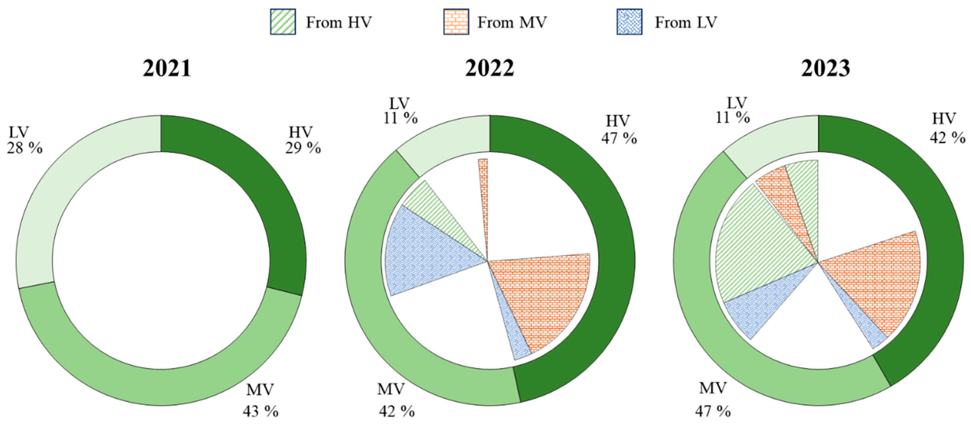
During the first year, the vigour reduction was almost zero, while 36% of plants showed an increase in vigour. Between the second and third year, despite pruning, during the 2023 growing season, the plants responded with intense vegetative growth, which allowed them to maintain the percentage distribution of vigour levels from the previous year. Overall, from July 2021 to July 2023, there was an increase in the number of HV plants and a decrease in LV plants, while the percentage of MV plants remained around 45% (Figure 14).
The ANOVA and Tukey’s test performed with a pvalue of 0.001 (Table 2) showed statistically significant differences in NDVI values between the first and third year of the experiment in the high and low vigour classes, while MV plants between the first and third years, on the other hand, did not show differences. Concerning the geometric conditions of vegetation, CA values for LV plants showed statistically significant differences across all the years, with higher values observed in the third year. In contrast, MV and HV plant groups in the second year of growth showed an increase in CA, while between the beginning and end of the two-year cycle (i.e., between 2021 and 2023), there were no statistically significant differences.
4. Discussion
The vegetative activity of trees can be modified through the agronomic management of various factors based on the vigour conditions of an olive orchard [37]. Therefore, the accurate assessment of the actual growth conditions is an essential element of appropriate, site-specific management. The assessment of olive trees’ geometric and spectral characteristics by processing images captured through multispectral cameras mounted on UAV platforms is feasible. This technology enables the high-resolution monitoring of plant health at various levels of detail and is an efficient alternative to laborious and expensive manual ground measurements [38]. In this experiment, NDVI showed a robust correlation with plant vigour, making it a valuable tool for assessing vegetation status. Consequently, any agronomic practice capable of modifying plant vigour can significantly impact the spectral response.
This study allowed us to evaluate the monitoring capability of an UAV with a multispectral camera in an intensive olive orchard subjected to biennial pruning. The correlation between the canopy area and volume measurements of individual plants and those estimated by UAV revealed the effectiveness of this technology, which is consistent with the findings of other studies [12,35,38]. Indeed, the correlations between the estimated and observed volumes were lower compared to those observed between the estimated and observed CAs (Figure 8). This discrepancy is caused by the inaccuracy of field measurements, especially in determining the average height of the canopy [26], as observed in other studies [12,38].
Furthermore, we observed that a smaller canopy size resulted in greater difficulty in estimating the geometric parameters. Therefore, larger and denser canopies allow for greater estimation accuracy with new survey technologies, including both algorithms and processing. This result emphasises the need for further studies to improve 3D model reconstructions in sparse canopies.
Biennial pruning can be the key to maintaining the vegetative and productive balance of plants [21]. Therefore, it should be calibrated based on the observed variability and requirements. In general, since, on average, more than 30% of the biomass was removed, the intervention carried out for the purposes of this experiment can be defined as intensive, as defined in Jiménez-Brenes et al. (2017) [21]. During the experiment, it was observed that plants underwent pruning based on their vigour level. Indeed, post- and pre-pruning volumes were correlated (Figure 11a) and the removed biomass statistically differed among the three vigour levels (Figure 10a). Furthermore, the removed biomass had a statistically different density depending on the vigour level. This effect can be explained by the different percentage ratio between leaves, the previous year’s branches and older branches. In fact, pruning density had statistically different values between high- and low-vigour trees (Figure 12), with higher values for high-vigour plants. This result, observed by Albarracín et al. (2017) [39] as well, highlights that the biomass removed from HV plants consisted of a higher percentage of old branches compared to leaves.
In general, pruning led to a reduction in the heterogeneity of the field, standardising the canopies in terms of their geometric (CA and CV) and consequently their spectral characteristics (Table 1). Therefore, biennial pruning was able to even out the geometric characteristics of the plants, allowing for the formation of vegetative and productive branches in the next year. This effect is favoured by the high plasticity of olive trees in responding to different levels of pruning, as observed by Rodrigues et al. (2018) [40], although the best response would be obtained with moderate intensities in the year after the intervention. If the plants were pruned with different intensities, and thus not according to their level of vigour, there would be an increase in spatial variability, making annual pruning necessary, as also observed by Farinelli et al. (2010) and Jiménez-Brenes et al. (2017) [21,41].
The 3D multi-temporal analysis of the olive grove models revealed the effect of pruning intensity on the annual growth of and spectral changes in the canopies. The years 2021 and 2022 allowed the plants to grow, resulting in an increase in size at all vigour levels. This allowed only 11.2% of the plants to be classified as low-vigour, according to the thresholds determined in the previous year. The increase in NDVI and CA values underlines the close association between these two parameters and plant growth [11,28]. Between the second and third year, pruning maintained 88.6% of the plants in the medium- to high-vigour levels. In general, comparing the starting and final conditions, HV and MV plants seem to have preserved their canopy surface and NDVI characteristics. In contrast, LV plants, having been pruned less and left to vegetate, showed an increase in CA and NDVI compared to the starting values. Overall, the experiment resulted in greater uniformity among the plants in the plot.
This study can be used as a starting point to investigate other aspects of olive cultivation. Indeed, a reduction in volume has a considerable impact on light penetration and light interception by the canopy [42]. These effects could be used to improve the actual estimation of irrigation requirements [18,43] or implement new growth models [22,44] or cultivar-specific models [24]. In addition, the amount of biomass can affect the efficiency of mechanical harvesting [23,45] and allow for using fewer pesticides for disease and pest control [46,47], especially if combined with greater precision in the estimation of canopy volumes [35]. The accurate quantification of the amounts of biomass that can be extracted from pruning can be useful for estimating energy production and may aid in the design of biomass energy plants [25,48]. Furthermore, for biomass left in the field, an accurate estimate of organic matter input can be obtained. This estimation allows for more appropriate choices on fertiliser distribution [19,49] and for a reduction in environmental impact [50].
5. Conclusions
This study was carried out over three years to obtain a complete overview of the possible implications of biennial pruning. UAVs, multispectral cameras, and OBIA techniques proved capable of assessing the effects of biennial pruning on canopy growth and the maintenance of plant vigour conditions. Intensive and progressively volume-based biennial pruning reduced the percentage of low-vigour plants, while maintaining stability and reducing differences between medium- and high-vigour plants. Pruning can therefore be differentiated based on vigour maps to maintain the correct vegetative and productive balance of plants. In addition, the experiment showed that remote sensing images and the OBIA approach were able to estimate biophysical parameters with high accuracy even in conditions of sparsely or dense canopies, significantly reducing costs and increasing estimation accuracy compared to manual assessments.
The results obtained come from the first study carried out in Sicily and can be implemented in other olive-growing areas with different cultivars, planting systems and pedoclimatic conditions.
Author Contributions
Conceptualisation, P.C. and M.V.; methodology, E.R. and S.O.; validation, E.R. and S.O.; formal analysis, E.R. and P.C.; investigation, E.R. and S.O.; resources, P.C. and M.V.; data curation, E.R. and P.C.; writing—original draft preparation, E.R. and M.V; writing—review and editing, P.C., S.O. and M.V.; visualisation, E.R. and S.O.; supervision, P.C. and M.V.; project administration, P.C. All authors have read and agreed to the published version of the manuscript.
Funding
This research was funded by the European Union—NextGenerationEU through the Italian Ministry of University and Research under PNRR within the project “SiciliAn MicronanOTecH Research And Innovation CEnter “SAMOTHRACE” (MUR, PNRR-M4C2, ECS_00000022), spoke 3—Università degli Studi di Palermo “S2-COMMs—Micro and Nanotechnologies for Smart & Sustainable Communities”. The views and opinions expressed are those of the authors only and do not necessarily reflect those of the European Union or the European Commission. Neither the European Union nor the European Commission can be held responsible for them.
Data Availability Statement
Data are contained within the article.
Conflicts of Interest
The authors declare no conflicts of interest.
References
- Godfray, H.C.J.; Beddington, J.R.; Crute, I.R.; Haddad, L.; Lawrence, D.; Muir, J.F.; Pretty, J.; Robinson, S.; Thomas, S.M.; Toulmin, C. Food Security: The Challenge of Feeding 9 Billion People. Science 2010, 327, 812–818. [Google Scholar] [CrossRef] [PubMed]
- Tilman, D.; Balzer, C.; Hill, J.; Befort, B.L. Global Food Demand and the Sustainable Intensification of Agriculture. Proc. Natl. Acad. Sci. USA 2011, 108, 20260–20264. [Google Scholar] [CrossRef] [PubMed]
- Faostat, F. Statistics, Food and Agriculture Organization of the United Nations, Rome. 2022. Available online: https://www.fao.org/faostat (accessed on 12 March 2024).
- Connor, D.J.; Gómez-del-Campo, M.; Rousseaux, M.C.; Searles, P.S. Structure, Management and Productivity of Hedgerow Olive Orchards: A Review. Sci. Hortic. 2014, 169, 71–93. [Google Scholar] [CrossRef]
- De Gennaro, B.; Notarnicola, B.; Roselli, L.; Tassielli, G. Innovative Olive-Growing Models: An Environmental and Economic Assessment. J. Clean. Prod. 2012, 28, 70–80. [Google Scholar] [CrossRef]
- Noori, O.; Panda, S.S. Site-Specific Management of Common Olive: Remote Sensing, Geospatial, and Advanced Image Processing Applications. Comput. Electron. Agric. 2016, 127, 680–689. [Google Scholar] [CrossRef]
- Perna, C.; Sarri, D.; Pagliai, A.; Priori, S.; Vieri, M. Assessment of Soil and Vegetation Index Variability in a Traditional Olive Grove: A Case Study; Springer: Berlin/Heidelberg, Germany, 2022; pp. 835–842. [Google Scholar]
- Sola-Guirado, R.R.; Castillo-Ruiz, F.J.; Jiménez-Jiménez, F.; Blanco-Roldan, G.L.; Castro-Garcia, S.; Gil-Ribes, J.A. Olive Actual “on Year” Yield Forecast Tool Based on the Tree Canopy Geometry Using UAS Imagery. Sensors 2017, 17, 1743. [Google Scholar] [CrossRef] [PubMed]
- Perna, C.; Pagliai, A.; Lisci, R.; Pinhero Amantea, R.; Vieri, M.; Sarri, D.; Masella, P. Relationship between Height and Exposure in Multispectral Vegetation Index Response and Product Characteristics in a Traditional Olive Orchard. Sensors 2024, 24, 2557. [Google Scholar] [CrossRef] [PubMed]
- Agam, N.; Segal, E.; Peeters, A.; Levi, A.; Dag, A.; Yermiyahu, U.; Ben-Gal, A. Spatial Distribution of Water Status in Irrigated Olive Orchards by Thermal Imaging. Precis. Agric. 2014, 15, 346–359. [Google Scholar] [CrossRef]
- Caruso, G.; Zarco-Tejada, P.J.; González-Dugo, V.; Moriondo, M.; Tozzini, L.; Palai, G.; Rallo, G.; Hornero, A.; Primicerio, J.; Gucci, R. High-Resolution Imagery Acquired from an Unmanned Platform to Estimate Biophysical and Geometrical Parameters of Olive Trees under Different Irrigation Regimes. PLoS ONE 2019, 14, e0210804. [Google Scholar] [CrossRef]
- Catania, P.; Roma, E.; Orlando, S.; Vallone, M. Evaluation of Multispectral Data Acquired from UAV Platform in Olive Orchard. Horticulturae 2023, 9, 133. [Google Scholar] [CrossRef]
- Díaz-Varela, R.A.; De la Rosa, R.; León, L.; Zarco-Tejada, P.J. High-Resolution Airborne UAV Imagery to Assess Olive Tree Crown Parameters Using 3D Photo Reconstruction: Application in Breeding Trials. Remote Sens. 2015, 7, 4213–4232. [Google Scholar] [CrossRef]
- Xie, Q.; Huang, W.; Liang, D.; Chen, P.; Wu, C.; Yang, G.; Zhang, J.; Huang, L.; Zhang, D. Leaf Area Index Estimation Using Vegetation Indices Derived from Airborne Hyperspectral Images in Winter Wheat. IEEE J. Sel. Top. Appl. Earth Obs. Remote Sens. 2014, 7, 3586–3594. [Google Scholar] [CrossRef]
- Xue, J.; Su, B. Significant Remote Sensing Vegetation Indices: A Review of Developments and Applications. J. Sens. 2017, 2017, 1353691. [Google Scholar] [CrossRef]
- Rouse, J.W.; Haas, R.H.; Schell, J.A.; Deering, D.W.; Harlan, J.C. Monitoring the Vernal Advancement and Retrogradation (Green Wave Effect) of Natural Vegetation. NASA/GSFC Type III Final. Rep. Greenbelt Md 1974, 371. Available online: https://ntrs.nasa.gov/citations/19740022555 (accessed on 12 March 2024).
- Carlson, T.N.; Ripley, D.A. On the Relation between NDVI, Fractional Vegetation Cover, and Leaf Area Index. Remote Sens. Environ. 1997, 62, 241–252. [Google Scholar] [CrossRef]
- Ben-Gal, A.; Agam, N.; Alchanatis, V.; Cohen, Y.; Yermiyahu, U.; Zipori, I.; Presnov, E.; Sprintsin, M.; Dag, A. Evaluating Water Stress in Irrigated Olives: Correlation of Soil Water Status, Tree Water Status, and Thermal Imagery. Irrig. Sci. 2009, 27, 367–376. [Google Scholar] [CrossRef]
- Roma, E.; Laudicina, V.A.; Vallone, M.; Catania, P. Application of Precision Agriculture for the Sustainable Management of Fertilization in Olive Groves. Agronomy 2023, 13, 324. [Google Scholar] [CrossRef]
- Martinez-Guanter, J.; Agüera, P.; Agüera, J.; Pérez-Ruiz, M. Spray and Economics Assessment of a UAV-Based Ultra-Low-Volume Application in Olive and Citrus Orchards. Precis. Agric. 2020, 21, 226–243. [Google Scholar] [CrossRef]
- Jiménez-Brenes, F.M.; López-Granados, F.; De Castro, A.; Torres-Sánchez, J.; Serrano, N.; Peña, J. Quantifying Pruning Impacts on Olive Tree Architecture and Annual Canopy Growth by Using UAV-Based 3D Modelling. Plant Methods 2017, 13, 55. [Google Scholar] [CrossRef]
- Villalobos, F.; Testi, L.; Hidalgo, J.; Pastor, M.; Orgaz, F. Modelling Potential Growth and Yield of Olive (Olea Europaea L.) Canopies. Eur. J. Agron. 2006, 24, 296–303. [Google Scholar] [CrossRef]
- Ferguson, L.; Glozer, K.; Crisosto, C.; Rosa, U.; Castro-Garcia, S.; Fichtner, E.; Guinard, J.; Lee, S.; Krueger, W.; Miles, J. Improving Canopy Contact Olive Harvester Efficiency with Mechanical Pruning. In Proceedings of the I International Symposium on Mechanical Harvesting and Handling Systems of Fruits and Nuts, Lake Alfred, FL, USA, 1–4 April 2012; pp. 83–87. [Google Scholar]
- Caruso, G.; Palai, G.; Marra, F.P.; Caruso, T. High-Resolution UAV Imagery for Field Olive (Olea Europaea L.) Phenotyping. Horticulturae 2021, 7, 258. [Google Scholar] [CrossRef]
- Velázquez-Martí, B.; Fernández-González, E.; López-Cortés, I.; Salazar-Hernández, D.M. Quantification of the Residual Biomass Obtained from Pruning of Trees in Mediterranean Olive Groves. Biomass Bioenergy 2011, 35, 3208–3217. [Google Scholar] [CrossRef]
- Miranda-Fuentes, A.; Llorens, J.; Gamarra-Diezma, J.L.; Gil-Ribes, J.A.; Gil, E. Towards an Optimized Method of Olive Tree Crown Volume Measurement. Sensors 2015, 15, 3671–3687. [Google Scholar] [CrossRef] [PubMed]
- Rosell, J.; Sanz, R. A Review of Methods and Applications of the Geometric Characterization of Tree Crops in Agricultural Activities. Comput. Electron. Agric. 2012, 81, 124–141. [Google Scholar] [CrossRef]
- Jurado, J.M.; Ortega, L.; Cubillas, J.J.; Feito, F. Multispectral Mapping on 3D Models and Multi-Temporal Monitoring for Individual Characterization of Olive Trees. Remote Sens. 2020, 12, 1106. [Google Scholar] [CrossRef]
- Kottek, M.; Grieser, J.; Beck, C.; Rudolf, B.; Rubel, F. World Map of the Köppen-Geiger Climate Classification Updated. Meteorol. Z. 2006, 15, 259–263. [Google Scholar] [CrossRef]
- Roma, E.; Catania, P.; Vallone, M.; Orlando, S. Unmanned Aerial Vehicle and Proximal Sensing of Vegetation Indices in Olive Tree (Olea Europaea). J. Agric. Eng. 2023, 54. [Google Scholar] [CrossRef]
- Catania, P.; Comparetti, A.; Febo, P.; Morello, G.; Orlando, S.; Roma, E.; Vallone, M. Positioning Accuracy Comparison of GNSS Receivers Used for Mapping and Guidance of Agricultural Machines. Agronomy 2020, 10, 924. [Google Scholar] [CrossRef]
- QGIS. Geographic Information System. 2022. Available online: https://www.qgis.org/it/site/ (accessed on 1 January 2022).
- Blaschke, T. Object Based Image Analysis for Remote Sensing. ISPRS J. Photogramm. Remote Sens. 2010, 65, 2–16. [Google Scholar] [CrossRef]
- RStudio Team. RStudio: Integrated Development Environment for R; RStudio Team: Boston, MA, USA, 2015. [Google Scholar]
- Anifantis, A.S.; Camposeo, S.; Vivaldi, G.A.; Santoro, F.; Pascuzzi, S. Comparison of UAV Photogrammetry and 3D Modeling Techniques with Other Currently Used Methods for Estimation of the Tree Row Volume of a Super-High-Density Olive Orchard. Agriculture 2019, 9, 233. [Google Scholar] [CrossRef]
- Zarco-Tejada, P.J.; Diaz-Varela, R.; Angileri, V.; Loudjani, P. Tree Height Quantification Using Very High Resolution Imagery Acquired from an Unmanned Aerial Vehicle (UAV) and Automatic 3D Photo-Reconstruction Methods. Eur. J. Agron. 2014, 55, 89–99. [Google Scholar] [CrossRef]
- Barranco-Navero, D.; Fernandez Escobar, R.; Rallo Romero, L. El Cultivo Del Olivo, 7th ed.; Mundi-Prensa Libros: Madrid, Spain, 2017; ISBN 84-8476-714-0. [Google Scholar]
- Torres-Sánchez, J.; López-Granados, F.; Serrano, N.; Arquero, O.; Peña, J.M. High-Throughput 3-D Monitoring of Agricultural-Tree Plantations with Unmanned Aerial Vehicle (UAV) Technology. PLoS ONE 2015, 10, e0130479. [Google Scholar] [CrossRef] [PubMed]
- Albarracín, V.; Hall, A.J.; Searles, P.S.; Rousseaux, M.C. Responses of Vegetative Growth and Fruit Yield to Winter and Summer Mechanical Pruning in Olive Trees. Sci. Hortic. 2017, 225, 185–194. [Google Scholar] [CrossRef]
- Rodrigues, M.Â.; Lopes, J.I.; Ferreira, I.Q.; Arrobas, M. Olive Tree Response to the Severity of Pruning. Turk. J. Agric. For. 2018, 42, 103–113. [Google Scholar] [CrossRef]
- Farinelli, D.; Onorati, L.; Ruffolo, M.; Tombesi, A. Mechanical Pruning of Adult Olive Trees and Influence on Yield and on Efficiency of Mechanical Harvesting. In Proceedings of the XXVIII International Horticultural Congress on Science and Horticulture for People (IHC2010): Olive Trends Symposium, Lisbon, Portugal, 22 August 2010; pp. 203–209. [Google Scholar]
- Castillo-Ruiz, F.J.; Castro-Garcia, S.; Blanco-Roldan, G.L.; Sola-Guirado, R.R.; Gil-Ribes, J.A. Olive Crown Porosity Measurement Based on Radiation Transmittance: An Assessment of Pruning Effect. Sensors 2016, 16, 723. [Google Scholar] [CrossRef]
- Lo Bianco, R.; Carella, A.; Massenti, R. Testing Effects of Vapor Pressure Deficit on Fruit Growth: A Comparative Approach Using Peach, Mango, Olive, Orange, and Loquat. Front. Plant Sci. 2023, 14, 1294195. [Google Scholar]
- Allen, W.A.; Richardson, A.J. Interaction of Light with a Plant Canopy. JOSA 1968, 58, 1023–1028. [Google Scholar] [CrossRef]
- Tombesi, A.; Boco, M.; Pilli, M.; Farinelli, D. Influence of Canopy Density on Efficiency of Trunk Shaker on Olive Mechanical Harvesting. In Proceedings of the IV International Symposium on Olive Growing, Valenzano, Italy, 25–30 September 2000; pp. 291–294. [Google Scholar]
- Miranda-Fuentes, A.; Llorens, J.; Rodríguez-Lizana, A.; Cuenca, A.; Gil, E.; Blanco-Roldán, G.; Gil-Ribes, J. Assessing the Optimal Liquid Volume to Be Sprayed on Isolated Olive Trees According to Their Canopy Volumes. Sci. Total Environ. 2016, 568, 296–305. [Google Scholar] [CrossRef]
- Planas, S.; Román, C.; Sanz, R.; Rosell-Polo, J.R. Bases for Pesticide Dose Expression and Adjustment in 3D Crops and Comparison of Decision Support Systems. Sci. Total Environ. 2022, 806, 150357. [Google Scholar] [CrossRef]
- Orlando, S.; Greco, C.; Tuttolomondo, T.; Leto, C.; Cammalleri, I.; La Bella, S. Identification of Energy Hubs for the Exploitation of Residual Biomass in an Area of Western Sicily. In Proceedings of the EUBCE 2017 Online Conference Proceedings, Stockholm, Sweden, 12–15 June 2017; pp. 64–69. [Google Scholar]
- Fernández-Escobar, R.; Marín, L. Nitrogen Fertilization in Olive Orchards. In Proceedings of the III International Symposium on Olive Growing, Chania, Crete, Greece, 22–26 September 1997; pp. 333–336. [Google Scholar]
- Van Evert, F.K.; Gaitán-Cremaschi, D.; Fountas, S.; Kempenaar, C. Can Precision Agriculture Increase the Profitability and Sustainability of the Production of Potatoes and Olives? Sustainability 2017, 9, 1863. [Google Scholar] [CrossRef]
Figure 1.
Experimental site location in the Mediterranean area and on the island of Sicily, Italy. Mean olive oil production calculated using FAOSTAT (2022) [3] data from 2018 to 2022.
Figure 1.
Experimental site location in the Mediterranean area and on the island of Sicily, Italy. Mean olive oil production calculated using FAOSTAT (2022) [3] data from 2018 to 2022.
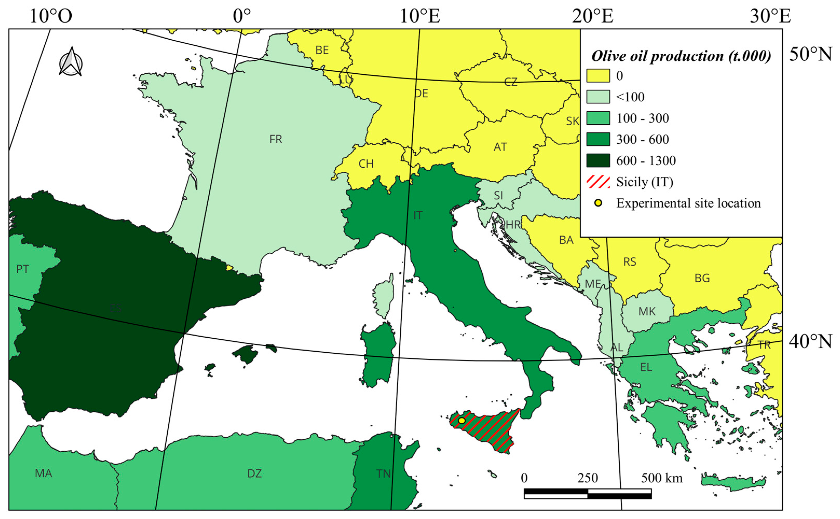
Figure 2.
Schedule of flights based on the BBCH stage of olive trees during this experimental study.
Figure 2.
Schedule of flights based on the BBCH stage of olive trees during this experimental study.

Figure 3.
Ground Control Points (GCP) in the experimental plot.
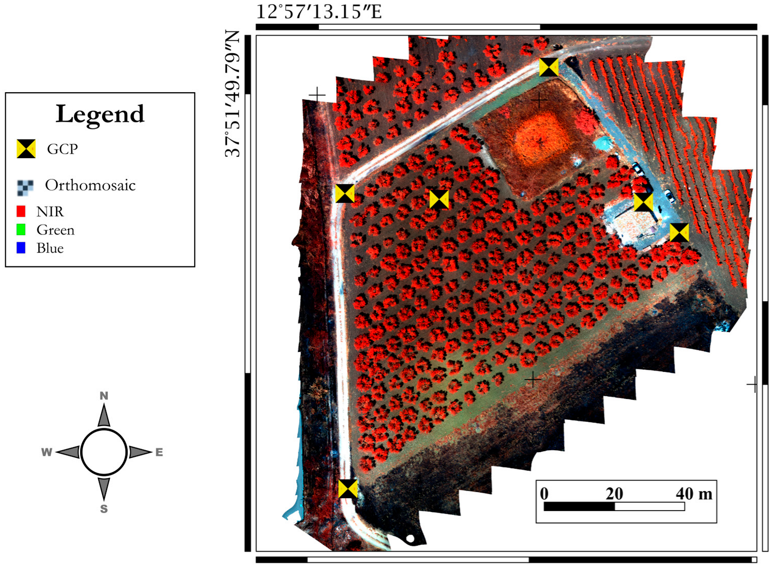
Figure 4.
Workflow of photogrammetry data processing.
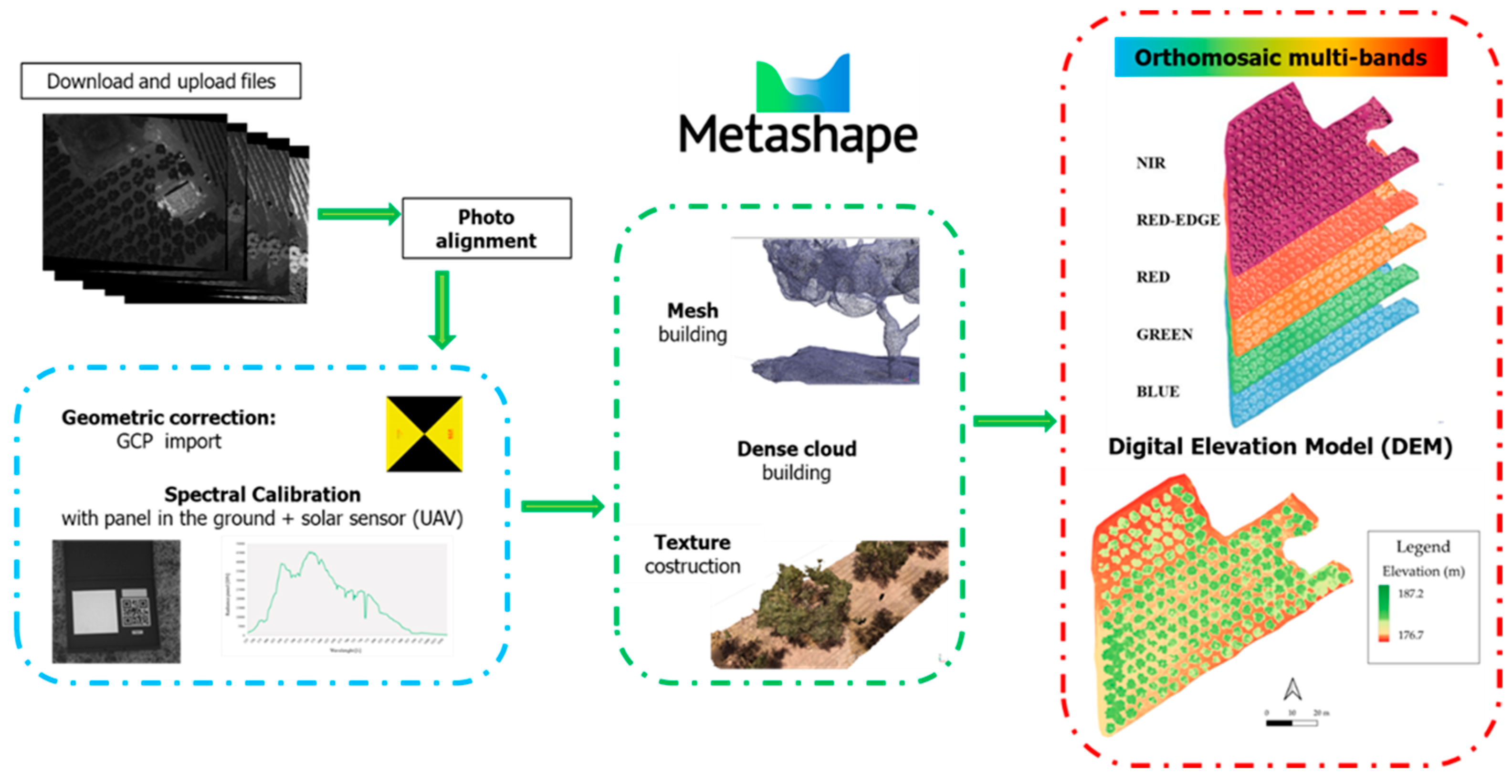
Figure 5.
Schematic representation of data processing input and output.
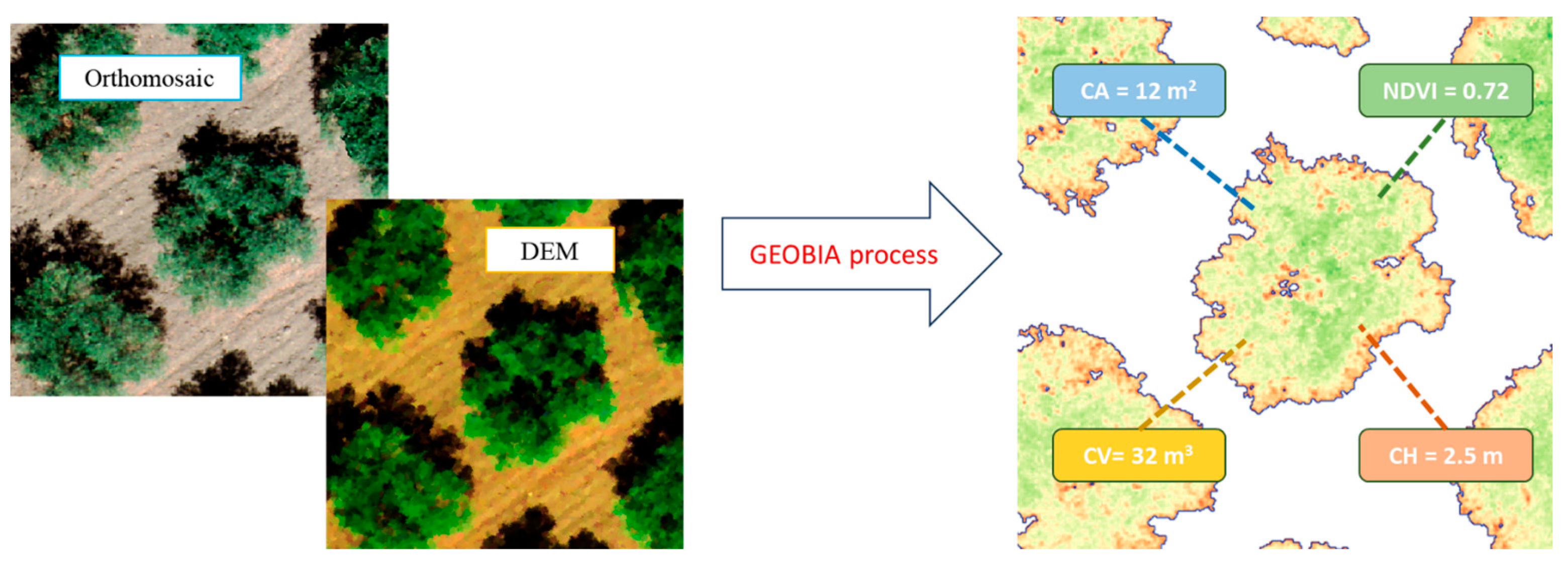
Figure 6.
Representation of canopies in RGB visualisation for the three vigour groups.
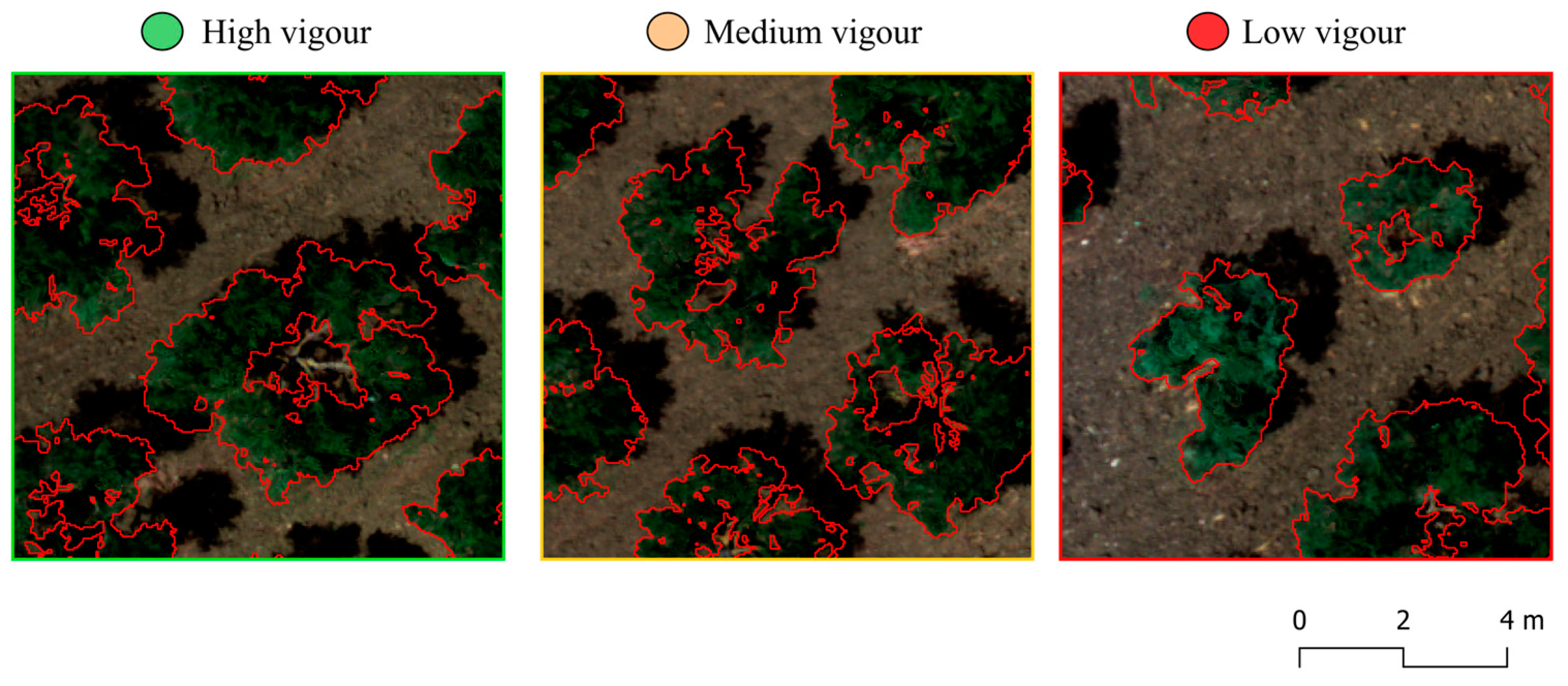
Figure 7.
Canopy height (CH) measurement on the sample plants and indication of the two main axes of the canopy (green and yellow colour represent vegetation and axes, respectively).
Figure 7.
Canopy height (CH) measurement on the sample plants and indication of the two main axes of the canopy (green and yellow colour represent vegetation and axes, respectively).
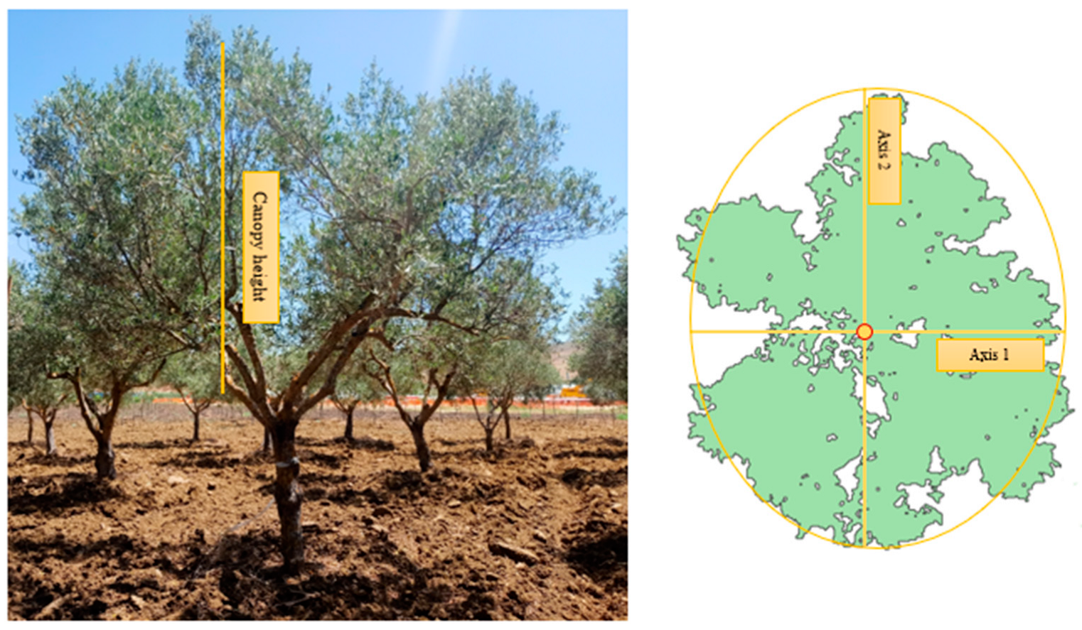
Figure 8.
Comparison between the observed and predicted values of canopy area (CA, m2) before (a) and after (b) pruning, canopy volume (CV, m3) before (c) and after (d) pruning and canopy height (CH, m) before (e) and after (f) pruning. The red line is the line interpolating the data. Green and yellow triangles represent the values obtained during the pre and post-pruning operation respectively for each plant.

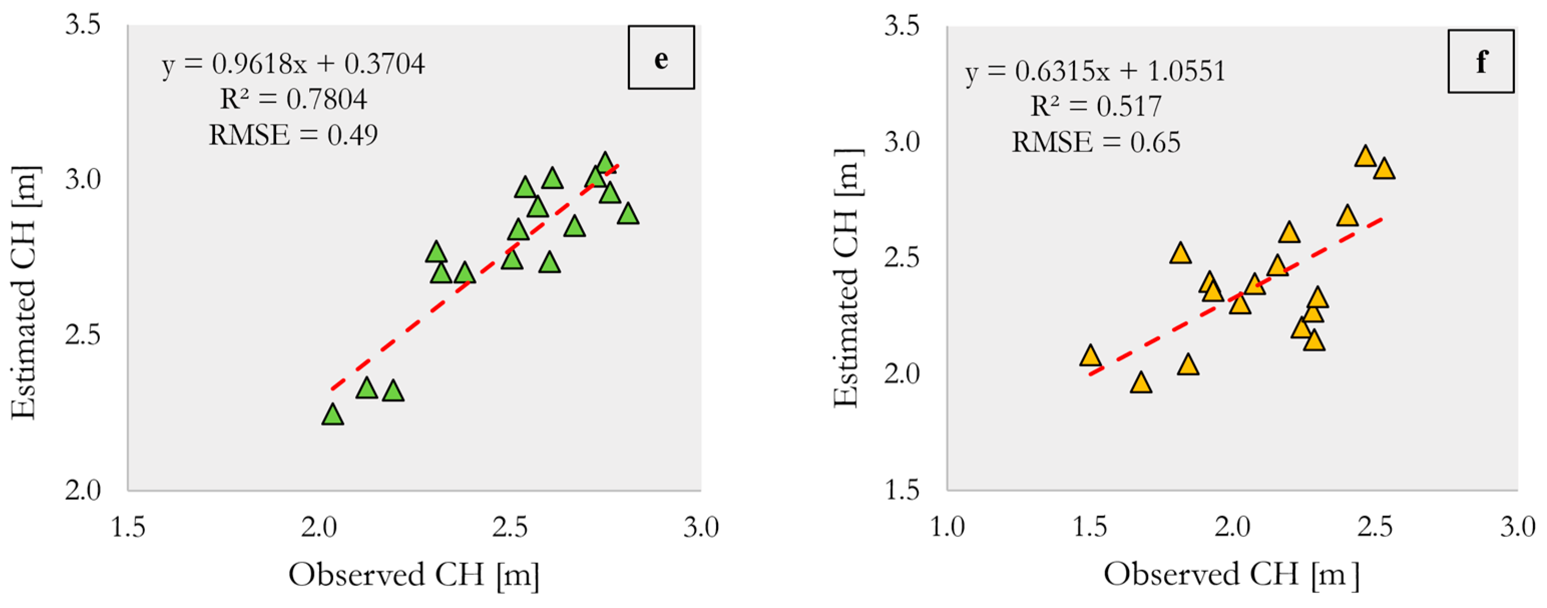
Figure 9.
Geometric variation of the canopy plant of a sample tree due to pruning in 3D and 2D view.
Figure 9.
Geometric variation of the canopy plant of a sample tree due to pruning in 3D and 2D view.
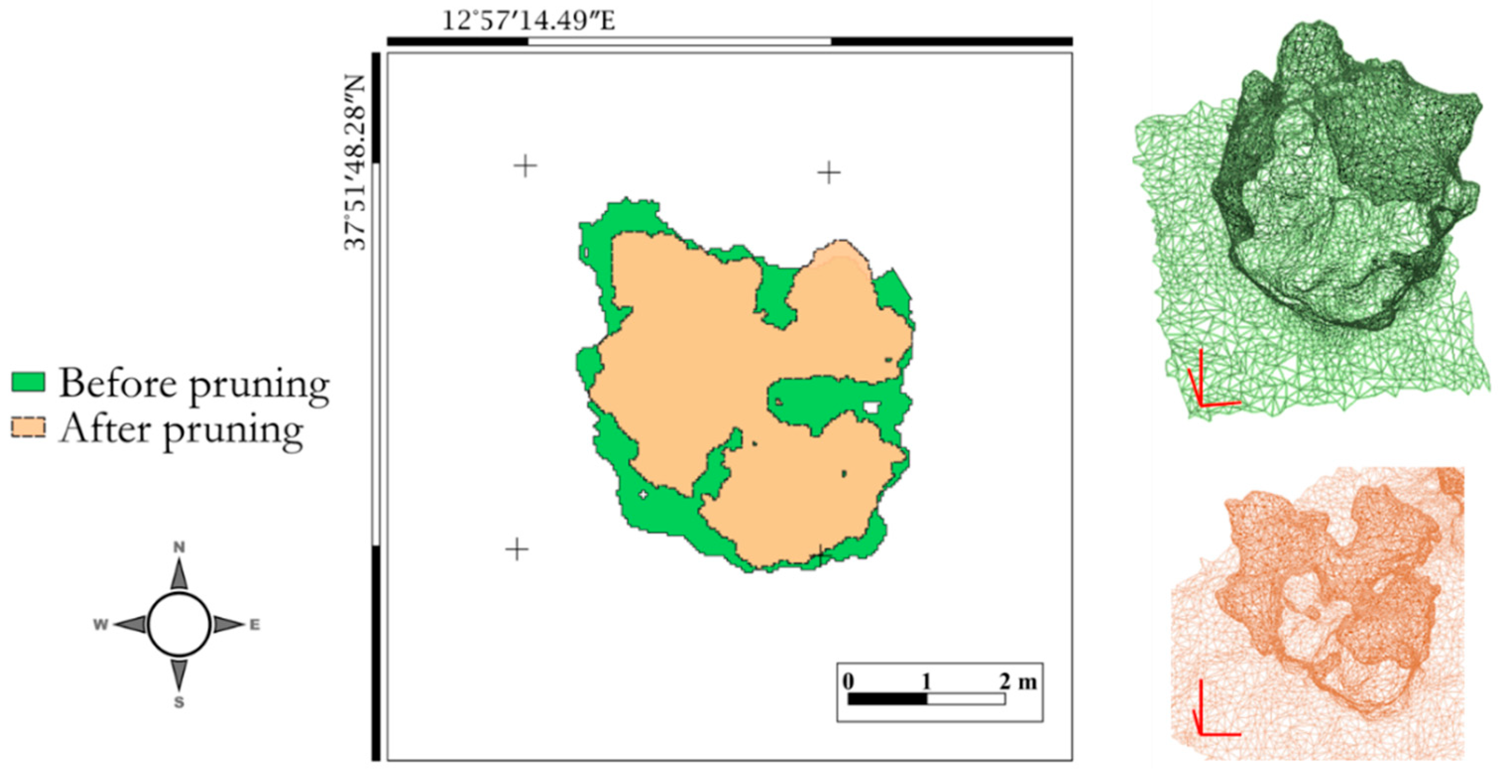
Figure 10.
(a) Biomass removed with pruning in the three vigour levels. (b) Correlation between volume and canopy area variation. The different bars colours represent the three vigour levels of the plants. Letters ‘a’, ‘b’, and ‘c’ indicate statistically significant differences among the groups, while red line is the line interpolating the data.
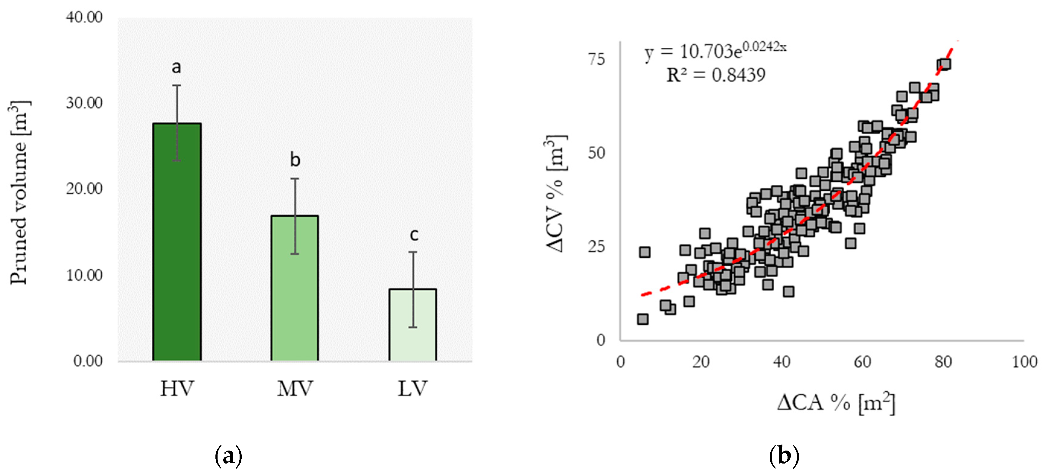
Figure 11.
(a) Correlation between volume before and after pruning in the 17 selected plants. (b) Correlation between ΔCV and pruning weight (kg). The red line is the line interpolating the data.
Figure 11.
(a) Correlation between volume before and after pruning in the 17 selected plants. (b) Correlation between ΔCV and pruning weight (kg). The red line is the line interpolating the data.
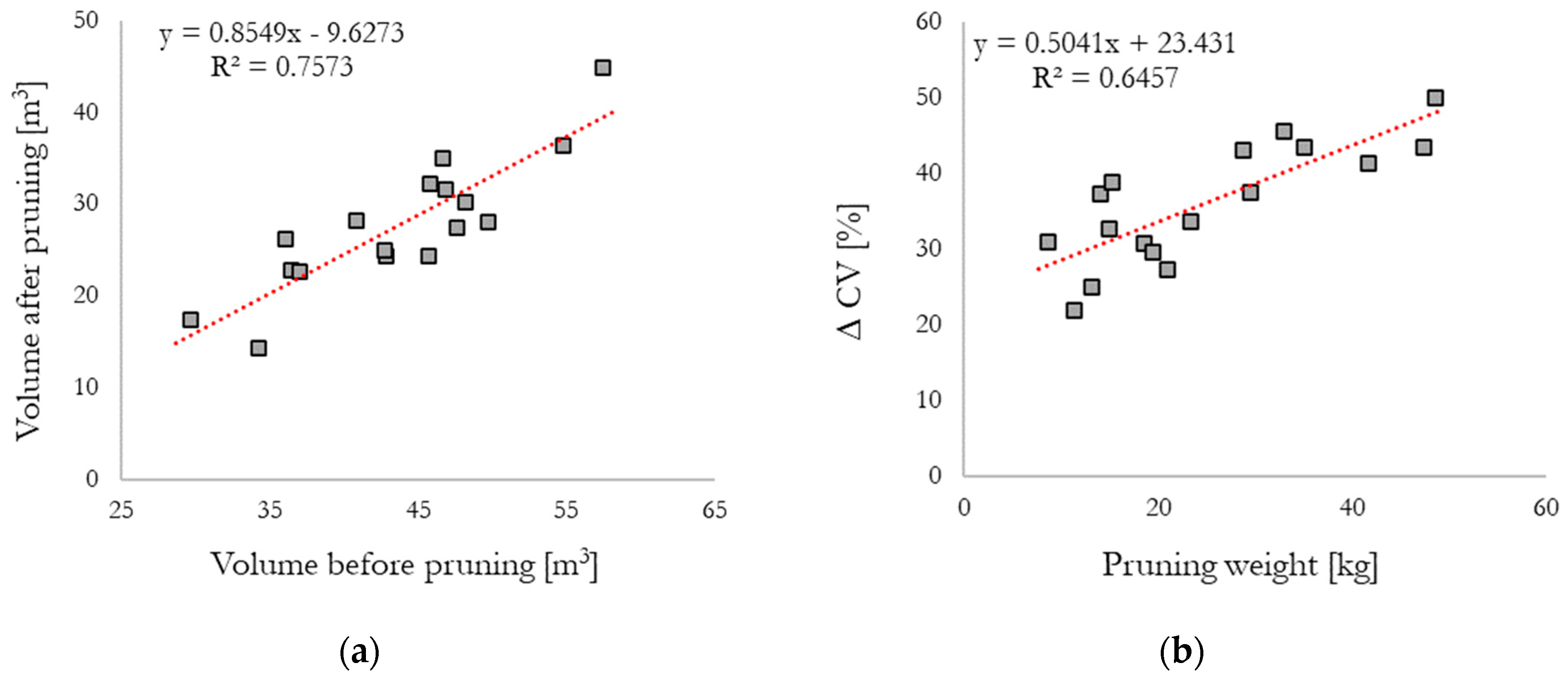
Figure 12.
(a) Biomass pruning density removed in the three vigour levels. (b) Correlation between pruning biomass and pruning density in the 17 selected plants. The different colours of the triangles and bars represent the three vigour levels of the plants. Letters ‘a’, ‘b’, and ‘c’ indicate statistically significant differences among the groups, while the red line is the line interpolating the data.
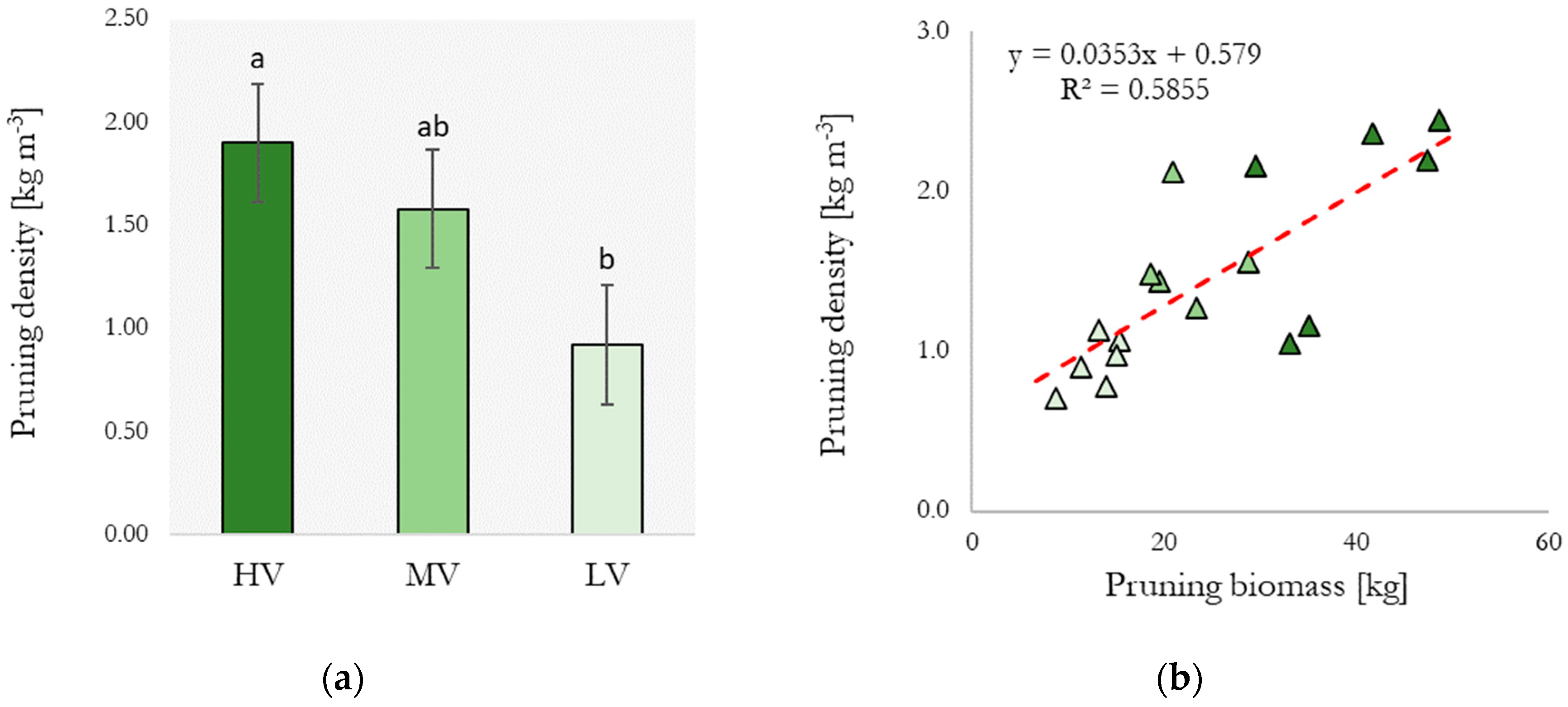
Figure 13.
Distribution of all plants in the three levels of vigour over the three-year experimental period, evaluated at the BBCH74 phenological stage.
Figure 13.
Distribution of all plants in the three levels of vigour over the three-year experimental period, evaluated at the BBCH74 phenological stage.

Figure 14.
Vigour levels percentage distribution observed over the three years (HV, MV, LV). Internal pie charts show percentage changes between one level of vigour and the others.
Figure 14.
Vigour levels percentage distribution observed over the three years (HV, MV, LV). Internal pie charts show percentage changes between one level of vigour and the others.

Table 1.
Results of ANOVA and Tukey’s test performed among the three vigour levels before and after pruning in terms of NDVI, CA and CV values (pvalue = 0.001). Letters ‘a’, ‘b’, and ‘c’ indicate statistically significant differences among the three groups HV, MV and LV.
Table 1.
Results of ANOVA and Tukey’s test performed among the three vigour levels before and after pruning in terms of NDVI, CA and CV values (pvalue = 0.001). Letters ‘a’, ‘b’, and ‘c’ indicate statistically significant differences among the three groups HV, MV and LV.
| Before | After | ||||
|---|---|---|---|---|---|
| Mean ± sd | Range | Mean ± sd | Range | ||
| NDVI | HV | 0.84 ± 0.02 a | 0.73–0.91 | 0.73 ± 0.04 a | 0.59–0.81 |
| MV | 0.81 ± 0.01 b | 0.75–0.83 | 0.74 ± 0.03 a | 0.62–0.81 | |
| LV | 0.78 ± 0.02 c | 0.72–0.82 | 0.71 ± 0.04 b | 0.64–0.79 | |
| CA | HV | 18.43 ± 2.3 a | 15.6–23.3 | 10.97 ± 2.7 a | 4.2–19.2 |
| [m2] | MV | 13.74 ± 1.0 b | 11.7–15.5 | 9.4 ± 1.8 ab | 4.9–13.1 |
| LV | 9.53 ± 2.3 c | 3.6–12 | 6.62 ± 1.9 b | 2.5–9.7 | |
| CV | HV | 54.10 ± 7.8 a | 54.1–72.3 | 26.38 ± 8.1 a | 10.0–34.9 |
| [m3] | MV | 38.3 ± 4.1 b | 30.6–45.1 | 21.10 ± 6.0 ab | 7.7–30.2 |
| LV | 23.94 ± 7.1 c | 12.0–31.1 | 15.55 ± 6.0 b | 5.1–27.9 | |
Table 2.
Results of ANOVA and Tukey’s test among the three years for NDVI and CA for each vigour level (p = 0.01). Letters ‘a’, ‘b’, and ‘c’ indicate statistically significant differences among the three groups HV, MV and LV.
Table 2.
Results of ANOVA and Tukey’s test among the three years for NDVI and CA for each vigour level (p = 0.01). Letters ‘a’, ‘b’, and ‘c’ indicate statistically significant differences among the three groups HV, MV and LV.
| HV | MV | LV | ||||
|---|---|---|---|---|---|---|
| NDVI | mean ± sd | Range | mean ± sd | Range | mean ± sd | Range |
| 2021 | 0.63 ± 0.02 b | 0.62–0.64 | 0.60 ± 0.03 b | 0.59–0.61 | 0.58 ± 0.03 c | 0.57–0.59 |
| 2022 | 0.67 ± 0.03 a | 0.66–0.68 | 0.65 ± 0.03 a | 0.64–0.65 | 0.63 ± 0.04 a | 0.62–0.64 |
| 2023 | 0.61 ± 0.03 c | 0.60–0.62 | 0.61 ± 0.03 b | 0.60–0.61 | 0.61 ± 0.03 b | 0.60–0.62 |
| CA | mean ± sd | Range | mean ± sd | Range | mean ± sd | Range |
| 2021 | 12.88 ± 2.1 b | 12.0–13.8 | 9.97 ± 0.86 b | 9.6–10.4 | 6.49 ± 1.60 c | 5.6–7.4 |
| 2022 | 14.92 ± 3.1 a | 14.0–15.8 | 12.28 ± 1.95 a | 11.9–12.7 | 9.04 ± 2.63 b | 8.1–9.9 |
| 2023 | 12.39 ± 2.8 b | 11.5–13.2 | 11.72 ± 0.48 ab | 9.7–13.7 | 11.70 ± 3.53 a | 10.8–12.6 |
Disclaimer/Publisher’s Note: The statements, opinions and data contained in all publications are solely those of the individual author(s) and contributor(s) and not of MDPI and/or the editor(s). MDPI and/or the editor(s) disclaim responsibility for any injury to people or property resulting from any ideas, methods, instructions or products referred to in the content. |
© 2024 by the authors. Licensee MDPI, Basel, Switzerland. This article is an open access article distributed under the terms and conditions of the Creative Commons Attribution (CC BY) license (https://creativecommons.org/licenses/by/4.0/).
Share and Cite
MDPI and ACS Style
Roma, E.; Catania, P.; Vallone, M.; Orlando, S. Assessing the Effectiveness of Pruning in an Olive Orchard Using a Drone and a Multispectral Camera: A Three-Year Study. Agronomy 2024, 14, 1023. https://doi.org/10.3390/agronomy14051023
AMA Style
Roma E, Catania P, Vallone M, Orlando S. Assessing the Effectiveness of Pruning in an Olive Orchard Using a Drone and a Multispectral Camera: A Three-Year Study. Agronomy. 2024; 14(5):1023. https://doi.org/10.3390/agronomy14051023
Chicago/Turabian StyleRoma, Eliseo, Pietro Catania, Mariangela Vallone, and Santo Orlando. 2024. "Assessing the Effectiveness of Pruning in an Olive Orchard Using a Drone and a Multispectral Camera: A Three-Year Study" Agronomy 14, no. 5: 1023. https://doi.org/10.3390/agronomy14051023
Note that from the first issue of 2016, this journal uses article numbers instead of page numbers. See further details here.