
Temporal and Spatial Assessment of Soil Salinity Post-Flood Irrigation: A Guide to Optimal Cotton Sowing Timing

1
Institute of Hydrogeology and Environmental Geology, Chinese Academy of Geological Sciences, Zhonghua Street 268, Shijiazhuang 050061, China
2
Key Laboratory of Groundwater Sciences and Engineering, Ministry of Natural Resources, Shijiazhuang 050061, China
3
Key Laboratory of Agricultural Soil and Water Engineering in Arid and Semiarid Areas, Ministry of Education, Northwest A&F University, Yangling 712100, China
4
State Key Laboratory of Biogeology and Environmental Geology & School of Environmental Studies, China University of Geosciences, Wuhan 430074, China
*
Author to whom correspondence should be addressed.
Agronomy 2023, 13(9), 2246; https://doi.org/10.3390/agronomy13092246
Submission received: 19 July 2023
/
Revised: 22 August 2023
/
Accepted: 24 August 2023
/
Published: 27 August 2023
(This article belongs to the Special Issue Improving Functioning of Soil–Plant Systems Using the Application of Sustainable and Intelligent Methods)
Abstract
:Flood irrigation is often applied in the arid regions of Northwest China to facilitate the leaching of salts accumulated in the soil during cotton growth in the previous season. This will, in turn, affect the temporal and spatial patterns of soil salinity, and thus cotton germination. To reveal the salinity of the two soil layers (0–20 cm and 20–60 cm), so as to determine the optimal cotton sowing timing, an electronic ground conductivity meter (EM38-MK2) was employed to measure the soil apparent electrical-conductivity (ECa) on different days: 4 days prior to flood irrigation, and, respectively, 6, 10, 15, 20, and 45 days after flood irrigation. Moreover, geostatistical analysis and block kriging interpolation were employed to analyze the spatial-temporal variations of soil salinity introduced by flood irrigation. Our results indicate that: (1) soil salinity in the two layers on different days can be well inverted from binary first-order equations of ECa at two coils (i.e., ECa1.0 and ECa0.5), demonstrating the feasibility of applying EM38-MK2 to estimate soil salinity in the field; and (2) soil salinity in the 0–20 cm layer significantly decreased during the first 15 days after flood irrigation with the greatest leaching rate of 88.37%, but tended to increase afterwards. However, the salinity in the 20–60 cm layer was persistently high before and after flood irrigation, with merely a brief decrease during the first 10 days after flood irrigation at the highest leaching rate of 40.74%. (3) The optimal semi-variance models illustrate that, after flood irrigation, the sill value (C0 + C) in the 0–20 cm layer decreased sharply, but the 20–60 cm Range of the layer significantly increased, suggesting that flood irrigation not only reduces the spatial variability of surface soil salinity, but also enhances spatial dependence in the 20–60 cm layer. (4) The correlation of the soil salinity between the two soil layers was very poor before flood irrigation, but gradually enhanced during the first 15 days after flood irrigation. Overall, for the study year, the first 15 days after flood irrigation was an optimal timing for cotton sowing when the leaching effects during flood irrigation were most efficient, and overrode the effects of evaporation and microtopography. Although not directly applicable to other years or regions, the electromagnetic induction surveys and spatiotemporal analysis of soil salinity can provide a rapid and viable guide to help determine optimal cotton sowing timing.
1. Introduction
Soil salinization caused by unsuitable irrigation seriously restricts the sustainable development of agriculture in arid and semi-arid areas [1]. For the areas short in freshwater resources, low-quality water (e.g., brackish water and reclaimed water) is often applied as irrigation water, which unfavorably introduces additional salt input [2,3]. For example, when brackish water (with salinity of 2–5 g L−1) was used under mulched drip irrigation in arid areas, salt accumulated in non-mulched belts due to limited infiltration depth and strong evaporation [3,4]. To amend localized soil salinization, flood irrigation is often applied between the two growth periods to leach salt out of the soil profile, preparing a low-salinity condition for the next growth period [5]. However, flood irrigation is highly susceptible to microtopography-induced variations, with lower terrains being more sufficiently leached than higher terrains. Therefore, apart from the benefits of leaching soil salt accumulated during previous growth period, it is equally critical to identify the additional spatial variations of soil salinity introduced by flood irrigation.
The spatial distribution of soil salinity is constantly evolving with specific conditions, such as soil texture and composition, precipitation and evaporation rate, groundwater level changes, and the duration of salt leaching after flood irrigation [6,7,8,9]. Therefore, accurately capturing the temporal and spatial patterns of soil salinity in the field is critically important when attempting to identify the best timing point for sowing. Considering that seed germination and emergence are particularly sensitive to top-soil salinity, the spatial patterns of localized salinization in the field can have long-lasting impacts on crop emergence and, later, the spatial distribution of the canopy. For instance, the tolerance threshold of cotton, one of the most common crops in the arid regions, to soil salinity (EC1:5) is 0.69 dS m−1 at seedling stage, and 1.02 dS m−1 at the flowering and bolling stage [10]. Therefore, to ensure crop emergence rate and the final crop yield, it is critically important to identify how intensively and persistently flood irrigation can affect the spatial variations of soil salinity before sowing [11].
Substantial studies have dedicated to investigating the spatial variations of soil salinity in the field, but they mostly relied on large number of sampling points, and exhaustive records on their temporal changes to evaluate the dynamics of soil salinization [12]. This often requires costly manpower, materials and time, if attempting to effectively capture the spatial variations of soil salinity in the field [13]. In recent years, non-contact remote sensing using satellites and drones have demonstrated significant advantages in salt risk assessment [14,15,16]. When integrated with geographic information technology, these methods enable rapid inversion of the spatiotemporal variations of salinity over a large scale, which can be employed to guide regional salinity management [17]. At the small-scale field, the non-contact electromagnetic induction investigation means, such as EM38, can efficiently complete the investigation of soil apparent conductivity (ECa) with more detailed soil information over a much shorter time [18,19,20]. Multiple linear regression, empirical coefficient, and other methods were used to convert ECa to soil salinity [18]. By calibrating ECa with a small number of measured soil salt contents at different depths, it can reveal the spatial distribution of soil salinity within each soil layer, as well as across different layers [21,22]. Consequently, compared to large-scale remote sensing methods, electromagnetic induction techniques exhibit advantages in terms of higher resolution, accuracy, and greater inversion depth when applied to the small-scale field.
In this study, we employed a ground conductivity meter (EM38-MK2) to capture and compare the spatial and temporal changes of oil salinity during non-growing period after flood irrigation. By geostatistical analysis of soil salinity variation and block kriging interpolation in the field, we attempted to prove the following hypotheses: (1) real-time calibrations were required for the field electromagnetic induction survey to effectively capture soil salinity on different days before and after flood irrigation; (2) flood irrigation can reconstruct the spatial pattern of soil salinity across the field, but spatial variability of soil salinity in different layers may not be synchronized; and (3) optimal timing for cotton sowing was dependent on the spatial and temporal variations of soil salinity over time.
2. Materials and Methods
2.1. Study Site
The study site (86°10′ E, 35°41′ N; 900 m a.s.l.) was located on an alluvial plain (900 m a.s.l.) of the Peacock River in the Tarim Basin in southern Xinjiang [23,24]. The region was characterized by low average annual precipitation (58.6 mm) and high annual evaporation rates (maximum potential evaporation is 2788 mm). Annual average temperature was 11.5 °C, ranging from −30.9 to 42.2 °C [24]. The experimental field was cropped with cotton. Soil type was loam soil, containing 46.81% sand, 45.96% silt and 7.23% clay. The average soil bulk density was 1.63 g cm−3. During the cotton growth period, brackish groundwater with a total dissolved solids (TDS) content of 2.4 g L−1 h used for mulched drip irrigation since 2008. Before cotton sowing, the field was often flooded with fresh surface water from reservoirs to help leach the salt that accumulated during the previous growth period. The groundwater table was approximately 5.8 m below the surface in 2016, thus having only limited impacts on salinity in the soil layer deep to 60 cm.
2.2. Experimental Design
From 29–30 April 2016 (before the growing season), the experimental field was flood-irrigated by 300 mm fresh water with a TDS content of 0.6 g L−1, following local irrigation practices (ranging between 225 mm and 315 mm) [25]. The experiment field was 10 m × 15 m, bordered by 25 cm high ridges (Figure 1). During the flood irrigation period, the daily average potential evaporation increased from 3.0 mm in April, to 3.8 mm in May, and to 5.8 mm in June, resulting in a cumulative evaporation of 386.2 mm. Meanwhile, the cumulative precipitation was merely 31.7 mm with a single maximum precipitation of 13.1 mm. The great ratio of evaporation–precipitation (i.e., 12.2), suggests high risks of evaporation-induced resalinization, but has limited effects by the way of precipitation-induced salt leaching. Thus, it is a typical field where the soil salinity and cotton sowing timing are dominantly regulated by irrigation practices, rather than natural precipitation. All the meteorological data were collected by Davis Vantage Pro 2 (Davis Instruments, Hayward, CA, USA).
A ground conductivity meter (EM38-MK2, Geonics Ltd., Mississauga, ON, Canada) was employed to measure ECa on different days: 4 days prior to flood irrigation (B-4), and 6, 10, 15, 20, and 45 days after flood irrigation (hereafter, respectively termed as A-6, A-10, A-15, A-20, and A-45). A total of 30 sampling points were evenly distributed across the experimental field (Figure 1). At each sampling point, soil samples were collected from two layers, 0–20 cm and 20–60 cm, and then were measured to determine the actual soil salinity, so as to establish inversion models with the ECa. Then, the inverted soil salinity was fitted to semi-variance functions to determine the effects of structural and random factors in the spatial variations of soil salinity [26,27]. Afterwards, to obtain the spatial distribution of soil salinity over the entire experimental field, the block kriging method was cross-validated and then applied using GS+ software (version 10.0.) to interpolate soil salinity values at locations that were not sampled by EM38-MK2 [28].
The 0–20 cm soil layer represented the key layer influencing cotton germination, whilst the 20–60 cm soil layer reflected the potential effects of cotton growth and root expansion at the post-seedling stage. The upper 60 cm was also the soil layer that was mostly affected by drip irrigation during the precedent growth period, where the wetting front often extended no deeper than 60 cm [11]. Since this study was to identify the optimal timing for cotton sowing based on the spatial and temporal variations of soil salinity after flood irrigation, no crops were planted for this season.
2.3. Electromagnetic Induction Survey
The EM38-MK2 used in this study can reach a depth of 1.5 m and a width of 1.0 m. It was equipped with two different coils, each of 0.5 and 1 m, which can simultaneously survey ECa0.5 and ECa1.0 in the vertical dipole mode. During each measurement day, the EM38-MK2 was lifted to cover the experimental field following predetermined routes, with 0.75 m space among individual survey lines (Figure 1c), each run completing approximately 3069~3441 times of data collection.
To verify the relationship between ECa and the soil salinity, 30 soil samples were collected on each measurement day. At each sampling point, the soil samples were collected at 0–20 cm and 20–60 cm using a soil borer. The collected soil samples were dried, milled, then mixed into suspension with the soil sample; a water ratio at 1:5 to measure electrical conductivity (EC1:5, mS cm−1) using a DDS-307 conductivity meter (Shanghai Yoke Instrument Co. Ltd., Shanghai, China) was used. In addition, 60 soil samples were randomly selected to measure soil salinity content (SSC, g kg−1), and then used to establish the relationship between SSC and EC1:5.
2.4. Geostatistical Analysis
Three types of semi-variance function models were applied to analyze the spatial variability of the soil salinity revealed from the EM38-MK2: spherical, Gaussian, and exponential model. The specific equations were as follows [29]:
Spherical Model:
Gaussian Model:
Exponential Model:
where γ(h) is the semi-variance for interval distance class h; h is the lag interval; C0 is the nugget variance (≥0); C is the structural variance (≥C0); a is the range for the spherical model (for Gaussian and exponential models, the ranges are and 3a, respectively).
The sill value (C0 + C) represents the variation caused by non-human regional factors (spatial autocorrelation part), which is the maximum variation of regionalized variables. Higher C0 + C means greater total spatial variation (Jiang, 2012) [30]. C0/(C0 + C) represents the relative contribution of random factor-induced spatial heterogeneity to the total spatial heterogeneity [11]. If C0/(C0 + C) < 25%, the variables have strong spatial dependence; if the ratio is between 25% and 75%, the spatial dependence of the variables is moderate; and if the ratio is >75%, the spatial dependence of the variables is weak [31,32]. The Range value reflects the influence range of regionalized variables: for a certain spatial interval, if the lag distance is shorter than the Range value, the variables are spatially dependent. When the lag distance (h) is greater than the Range value, the variables are independent of each other and then are then considered to spontaneous [29]. The GS+ software was employed to perform optimal semi-variogram fitting for soil salinity at different days and two layers.
The estimation of unknown locations is commonly achieved using kriging interpolation methods, with the fundamental equation as follows [33]:
where is the value to be estimated at the unknown location ; is the estimated value at the location, and is the unknown weight for the measured value at the location.
In this study, we employed the block kriging (with a local grid of 2 × 2) to interpolate the unknown locations, as the interpolation results of block kriging are smoother and provide better overall trends compared to ordinary kriging.
2.5. Soil Salinity Classification
Following the soil salinity classes of <2, 2–4, 4–6, 6–20, and >20 g kg−1, the inverted soil salinity was classified into 5 groups: non-salinized soil, slightly salinized soil, moderately salinized soil, heavy salinized soil, and saline soil [34]. The soil salinity data were transformed into isoline files and saved as the Surfer Grid (.grd) format. They were then imported into Surfer software (version 18.0), where the grid file was set as the upper surface, and the 5 salinity classes were, respectively, set as the lower surfaces. The assessment of soil salinization risks was conducted by determining the proportions (%) of different salinity classification areas relative to the total area of the field.
3. Results
3.1. Regressions between Soil Electrical Conductivity and Soil Salinity
The EC1:5 and SSC of the 60 selected soil samples were segment fitted (Figure 2); when EC1:5 ≤ 1 mS cm−1, the SSC were linearly correlated with the EC1:5 but the slope aspect was merely 2.94; when EC1:5 ≥ 1 mS cm−1, the SSC were also linearly correlated with the EC1:5 and the slope aspect was great at 9.04. The R2 and RMSE in both segments indicate that the linear correlations between EC1:5 and SSC were robust (Figure 2). Following the segment fittings between EC1:5 and SSC, the SSC of all the collected soil samples were obtained from their EC1:5 values.
Linear inversion models between the ECa (independent variable) and SSC (dependent variable) were established for the two soil layers on different measurement days (Table 1). For almost all the layers on different days, the correlations between the SSC and ECa were significant (p < 0.05), except for the 0–20 cm layer, 6 days after flood irrigation, which might be attributed to the pronounced heterogeneity in surface soil salinity, resulting from flood irrigation (Table 1). In addition, the interpretation accuracy of the 0–20 cm layers was lower than that of the 20–60 cm layers (Table 1). Furthermore, all the inversion models were functions of both ECa1.0 and ECa0.5, except for the 0–20 layer at 10 and 15 days after flood irrigation (Table 1). Therefore, the inversion model between the ECa and SSC can be generalized as:
where SSC is the soil salinity content (g kg−1); ECa1.0 and ECa0.5 are the soil apparent electrical conductivity corresponding to the 1.0 m and 0.5 m coil, respectively (mS cm−1); and a, b, and c are fitted coefficients or constants.
SSC = a ECa1.0 + b ECa0.5 + c
3.2. Optimal Semi-Variance Function Models of Soil Salinity
The coefficients of determination (R2), Residual Sum of Squares (RSS) and key parameters of the optimal semi-variance models for soil salinity in each layer on different days are listed in Table 2. The R2 values were above 0.95 for all the cases. The exponential model was the optimal semi-variance model for both layers before flood irrigation. The spherical model was most suitable for each surface layer (0–20 cm) after flood irrigation, except for A-20, where an exponential model fitted the best. Meanwhile, a Gaussian model fitted the best for all the deep layers (20–60 cm) after flood irrigation.
Specifically, for the 0–20 cm soil layer, the C0 + C declined sharply from 0.612 before flood irrigation to <0.011 after flood irrigation (Table 2). The C0/(C0 + C) for each layer was less than the spatial dependence threshold (25%), except for a slightly higher 25.38% in the 0–20 cm layer on A-20. The variations of C0/(C0 + C) suggest a relatively strong correlation in soil salinity, and structural factors predominated the spatial heterogeneity rather than the random factors. For the correlation length (Range), it varied between 8.28 m and 19.09 m in the 0–20 cm layer with no distinguished patterns before and after irrigation. However, in the 20–60 cm layer, the Range was 3.51 m before flood irrigation, and was consistently >10 m after flood irrigation (Table 2).
3.3. Spatial and Temporal Variations of Soil Salinity
The parameters of cross-validation of soil salinity distribution, following the optimal semi-variance models, are listed in Table 3. The determination coefficient R2 was greater than 0.8 (except for the 0–20 cm on A-20), and the SE was <0.01, suggesting that the spatial variability of soil salinity described by the optimal semi-variance models can be interpolated with high precision from the block kriging method. Moreover, compared to the 0–20 cm layer, the R2 of 20–60 cm was greater, and the SE was lower (Table 3).
After interpolation following the block kriging method, the soil salinity was unevenly distributed across the study plot between the two layers, and over different days (Figure 3). More specifically, the soil salinity of the two layers (0–20 cm and 20–60 cm) before irrigation was relatively high, then effectively leached by flood irrigation, and tended to increase afterwards. Local areas with lower terrain (i.e., the ponding area in Figure 1b) showed better leaching effects, and thus featured with relatively lower soil salinity after flood irrigation.
A statistical summary of the inverted soil salinity of the entire experimental plot is shown in Figure 4. In general, the soil salinity in the 0–20 cm layer was much less than that of the 20–60 cm layer, both of which decreased after flood irrigation and then increased with time. Specifically, for the 0–20 cm layer, the average soil salinity decreased sharply from 4.3 g kg−1 on B-4 to about 0.5 g kg−1 on A-6 (Figure 4a), illustrating a high desalination rate of 88.37%. The low soil salinity was preserved well afterwards and was steadily approaching 1.0 g kg−1 on A-45.
For the 20–60 cm layer, the average soil salinity before irrigation was about 27 g kg−1, and decreased significantly to about 16 g kg−1 on A-6 (Figure 4b), with an overall desalination rate of 40.74%. However, since A-15, the soil salt content tended to increase again, where the average soil salinity remained stable around 28 g kg−1 until A-45. In addition, compared to the 20–60 cm layer, the salt leaching of flood irrigation was much more effective in the 0–20 cm layer, resulting in much more stable and less varied soil salinity after irrigation (Figure 4a). In contrast, the soil salinity of the 20–60 layer showed strong spatial variability, which had even enlarged significantly since A-15 (Figure 4b).
3.4. Classification of Soil Salinity
Classified soil salt distributions [35] on different days are listed in Table 4, where the two soil layers distinctly differed from each other. For the 0–20 cm layer, 31.60% of the area was classified as slightly salinized soil, and 67.91% as moderately salinized soil before flood irrigation (B-4) (Table 4). After flood irrigation, all the soil in the 0–20 cm layer was leached to non-saline soil (100%), and such pattern lasted until A-45. This indicates that flood irrigation could achieve relatively uniform leaching of the topsoil in small-scale field plots, maintaining a low salt level for an extended period post-irrigation. Such an improvement in soil salinity was advantageous for ensuring a low-salinity soil environment, conducive to cotton germination.
For the 20–60 cm layer, 96.30% of the area was classified as saline soil before flood irrigation, but 91.17% was changed to heavily salinized soil after flood irrigation. This indicates that flood irrigation also had a significant leaching effect on soil salinity in the deeper layer. However, since A-15, most soil in the 20–60 cm layer was back to saline soil (91.24%), and was maintained until A-45 (82.57%) (Table 4). Notably, irrespective of before or after flood irrigation, the soil salinity in the 20–60 cm layer of the small-scale field plots remained consistently above the threshold for heavily salinized soil (Table 4). In contrast, the upper 0–20 cm layer did not exceed the threshold for moderately salinized soil (Table 4). Such persistent layer-specific patterns of soil salinity point to a pronounced trend of salt accumulation at the deeper layer (20–60 cm), which resulted from prolonged drip irrigation with brackish water during the growing season; this could not be overturned even after flood irrigation.
4. Discussion
4.1. Salinity Inversion Model Needs Real-Time Calibration
Soil salinity in the two layers on different days can be well inverted from binary first-order equations of apparent electrical conductivity ECa1.0 and ECa0.5, demonstrating the feasibility of applying EM38-MK2 to estimate soil salinity in the field. However, the specific parameters of the inversion models were different between the two soil layers, as well as among different measurement days, suggesting that all the inversion models must be calibrated with the actual SSC on each measurement day to ensure the accuracy. This was mostly because soil moisture changes can affect the apparent conductivity of EM38 [36,37], especially when infiltration and evaporation rates drastically changed before and after irrigation, as in this study. We acknowledge that other than soil salinity and moisture, the soil apparent conductivity can also capture and thus be interfered by the changes of other soil properties, such as texture [38], and compaction [39]. However, specifically for this study, soil texture and compaction were intrinsic properties with limited changes. Therefore, a real-time calibration during each survey could effectively eliminate the potential influences from soil moisture on the accuracy of soil salinity inversion. For different seasons in the same field, or in other fields with different soil texture or moisture content, real-time calibrations are always required. Overall, field investigations of soil salinity can be efficiently improved by combining the non-contact electromagnetic induction survey with a small number of calibrated samples, and thus have a greater potential to be widely applied in different regions [40].
4.2. Flood Irrigation Redistributed Soil Salinity across the Field
The optimal semi-variance models illustrate that, after flood irrigation, C0 + C in the 0–20 cm layer decreased sharply (Table 1), indicating that flood irrigation could reduce the intensity of spatial variability of surface soil salinity. As the salt leached from the surface soil entered in the 20–60 cm layer, the Range of 20–60 cm significantly increased (Table 2), suggesting a higher spatial dependence of soil salinity. Meanwhile, the soil salinity isolines, based on block kriging interpolation, tended to expand along the x-axis (e.g., south to north, Figure 3), which were consistent with the layout of the drip lines at the growth stage, as salt tends to accumulate at the edge of wet bodies [23,41]. This suggests that even flood irrigation with efficient leaching could not completely eliminate the salt distribution patterns shaped by the repeated drip irrigation during the previous growth period. Therefore, flood irrigation reshaped the distribution of soil salinity between the adjacent upper and lower layers, yet its impacts were also superimposed by the spatial variation of soil salinity formed during previous the growth period.
Furthermore, the significantly reduced soil salinity in the two layers (Figure 3 and Figure 4, and Table 4) clearly demonstrate the effectiveness of flood irrigation in terms of leaching soil salt and reducing soil salinity. However, such leaching effects were not uniform across the field; for the lower-lying terrain (the ponding part in Figure 1b), the soil salinity was significantly reduced by flood irrigation, and was persistently low until A-45 (Figure 3). For the higher lying terrain, the water depth was relatively small, resulting in insufficient salt leaching [11,12], and thus, more salt accumulation after evaporation. This further amplified the role of microtopography on soil salinity variation. Therefore, for salinized plots in arid areas, land levelling not only means easier farming, equal irrigation depth and water saving [42], but also, it is crucial to ensure comparable salt leaching, namely less nutrient loss by excessive leaching in lower-lying terrain, while less salt accumulation, by insufficient leaching and evaporation in higher lying terrain. Moreover, uneven salt leaching can be improved by irrigation modes. For example, drip irrigation may be adopted in non-growing period to help alleviate the effects of micro-topography on soil salinity variations with deformable pipelines, smaller water discharge, and thus better salt leaching effects [43].
4.3. Salinity Correlation between Surface and Deeper Layer Changed over Time
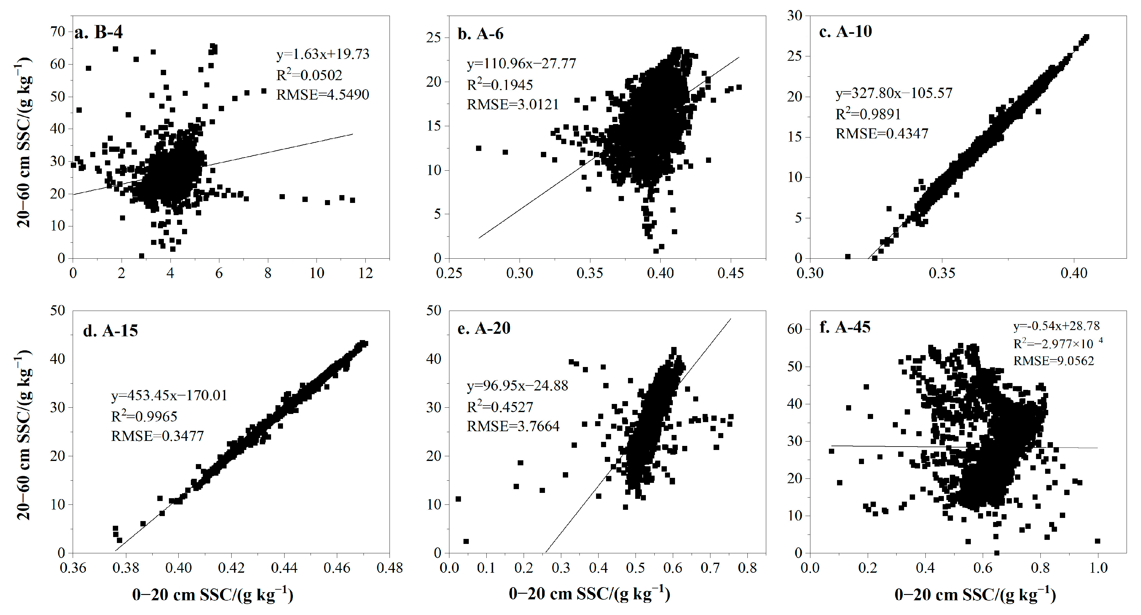
As a result of long-term mulched drip irrigation with brackish water, the soil salinity in the 20–60 cm layer was always much higher than that in the 0–20 cm (Figure 3, Figure 4 and Figure 5, Table 4). Since the drip irrigation depth during the growing season usually would not exceed 60 cm, and the salt tended to accumulate along the edges of the wetting bodies below the drippers [23], the 20~60 cm then became an area receiving the salt leached from the upper 0~20 cm. Meanwhile, the soil salinity in the 0–20 cm and 20–60 cm layer at the same survey point of EM-38 also appeared to correlate with each other (Figure 5). However, their correlation intensity changed strongly over time: before flood irrigation (i.e., before the growing season), the soil salinity in the two adjacent layers was poorly correlated (R2 = 0.05, Figure 5a), as soil evaporation and microtopography governed the soil salinity distribution [44,45]. After flood irrigation, the leaching effects synchronized the soil salinity in the two adjacent layers, strengthened their correlation, and the R2 of the linear relationship reached 0.99 on A-15 (Figure 5d). Afterwards, the effect of flood irrigation became weaker over time, while the effects of soil evaporation and microtopography became increasingly prominent. Hence, the spatial correlation became weaker until no linear correlation was observed on A-45 (Figure 5f).
4.4. Recommendation for Optimal Sowing Timing
Before flood irrigation, 97.3% area of the top 0–20 cm soil layer had soil salinity > 3 g kg−1, the threshold salinity for seedling emergence [46]. After flood irrigation, the soil salinity of all the top 0–20 cm soil layer was reduced to <2 g kg−1 on A-6, and such a low soil salinity class was maintained until A-45 (Table 4). However, it should be noted that, although classified as non-saline soil (Table 4), the soil salinity started to show resalinization since A-15 (Figure 3 and Figure 4). Meanwhile, the high salinity of 20–60 cm layer (6–20 g kg−1, Table 4) would also have a great potential influence on cotton growth, as the cotton roots gradually extended to the deep layer [3]. Therefore, the low soil salinity in 0–20 cm after flood irrigation, and its good synchronization with 20–60 cm from A-10 to A-15 (Figure 5), jointly recommend that cotton sowing should be not later than A-15. From the perspective of soil salinity, before A-15 was an optimal timing for cotton sowing, as the leaching effects during flood irrigation were most efficient by then, overriding the effects of evaporation and microtopography, hence ensured stably low soil salinity conditions for seeding. For other years or regions, with the help of the electromagnetic induction surveys and real-time calibrations, spatiotemporal analysis can be conducted rapidly and also viably. On applied side, other environmental factors, such as meteorology (temperature, precipitation, etc.) [47], groundwater quality [48] and evaporation [49], soil moisture [50], and farmers’ practices, should also be accounted for when choosing sowing timing. In particular, future studies should also consider the spatial variation and changes of precedent soil moisture [51]. For instance, when soil moisture falls back to the appropriate content after flood irrigation, mechanical tillage can be carried out first to destroy the capillary transport of water. Then, the dry soil layer formed on the surface layer can effectively prevent evaporation [52], hence reducing the secondary salinization otherwise caused by strong evaporation.
5. Conclusions
A ground conductivity meter was employed to survey the soil apparent electrical conductivity before and on different days after flood irrigation in a cotton field in a typical oasis in Northwest China. Soil salinity in the two layers (0–20 cm and 20–60 cm) was significantly reduced after flood irrigation by leaching, and their temporal variations over different days were well captured and inverted using real-time calibrated EM38-MK2. After analysis with semi-variance models and interpolation with the block kriging method, it was observed that flood irrigation not only reduces the spatial variability of surface soil salinity, but also enhances spatial dependence in the 20–60 cm layer. Meanwhile, the soil salinity isolines appeared to be consistent with the drip lines layout, further suggesting that flood irrigation cannot completely erase the salt distribution patterns shaped by the repeated drip irrigation during the previous growth period. Furthermore, the soil salinity in the two adjacent layers was poorly correlated before flood irrigation, but was significantly strengthened after flood irrigation, especially on the first 10 to 15 days after flood irrigation. It was collectively recommended that, if attempting to make a good use of soil conditions with reasonably low soil salinity, sowing should be conducted no later than the first 15 days after flood irrigation. The findings of this study not only confirm the feasibility of electromagnetic induction surveys and the spatiotemporal analysis of soil salinity, but also help to determine the optimal cotton sowing timing for the arid regions susceptible to salinization. However, we acknowledged that the spatial-temporal variations of soil salinity observed in the small-scale plot over one year cannot be directly extrapolated to a larger field or other years, where the interactions of soil water and salinity with soil texture and topography are far more complicated. Future studies should further investigate the potential impacts of land levelling, irrigation practices (e.g., drip irrigation during non-growing periods), soil texture, soil moisture, and their interactions in shaping the spatiotemporal variations of soil salinity and crop growth.
Author Contributions
Writing—original draft preparation, Y.H.; Methodology and investigation, X.L.; Supervision, M.J. All authors have read and agreed to the published version of the manuscript.
Funding
This research was funded by the National Natural Science Foundation of China, grant number 42272306 and 41502225; and the Fundamental Research Funds for the Central Universities, grant number 2452017191.
Data Availability Statement
Data of this research are available upon request to the corresponding author.
Conflicts of Interest
The authors declare no conflict of interest. The funders had no role in the design of the study; in the collection, analyses, or interpretation of data; in the writing of the manuscript; or in the decision to publish the results.
References
- Singh, A. Soil salinization management for sustainable development: A review. J. Environ. Manag. 2021, 277, 111383. [Google Scholar] [CrossRef]
- Liu, B.; Wang, S.; Kong, X.; Liu, X.; Sun, H. Modeling and assessing feasibility of long-term brackish water irriga-tion in vertically homogeneous and heterogeneous cultivated lowland in the North China Plain. Agric. Water Manag. 2019, 211, 98–110. [Google Scholar] [CrossRef]
- Chen, W.; Jin, M.; Ferré, T.P.A.; Liu, Y.; Xian, Y.; Shan, T.; Ping, X. Spatial distribution of soil moisture, soil salinity, and root density beneath a cotton field under mulched drip irrigation with brackish and fresh water. Field Crop. Res. 2018, 215, 207–221. [Google Scholar] [CrossRef]
- Li, X.; Jin, M.; Zhou, N.; Jiang, S.; Hu, Y. Inter-dripper variation of soil water and salt in a mulched drip irrigated cotton field: Advantages of 3-D modelling. Soil Tillage Res. 2018, 184, 186–194. [Google Scholar] [CrossRef]
- Wang, Z.; Jin, M.; Šimůnek, J.; Genuchten, M.T.V. Evaluation of mulched drip irrigation for cotton in arid Northwest China. Irrig. Sci. 2014, 32, 15–27. [Google Scholar] [CrossRef]
- Selim, T.; Bouksila, F.; Berndtsson, R.; Persson, M. Soil Water and Salinity Distribution under Different Treatments of Drip Irrigation. Soil Sci. Soc. Am. J. 2013, 77, 1144–1156. [Google Scholar] [CrossRef]
- Ortiz, A.C.; Jin, L. Chemical and hydrological controls on salt accumulation in irrigated soils of southwestern U.S. Geoderma 2021, 391, 114976. [Google Scholar] [CrossRef]
- Shokri-Kuehni, S.M.S.; Raaijmakers, B.; Kurz, T.; Or, D.; Helmig, R.; Shokri, N. Water table depth and soil salinization: From pore-scale processes to field-scale responses. Water Resour. Res. 2020, 56, e2019WR026707. [Google Scholar]
- Liu, Q.; Mou, X.; Cui, B.; Ping, F. Regulation of drainage canals on the groundwater level in a typical coastal wet-lands. J. Hydrol. 2017, 555, 463–478. [Google Scholar] [CrossRef]
- Che, Z.; Wang, J.; Li, J. Determination of threshold soil salinity with consideration of salinity stress alleviation by applying nitrogen in the arid region. Irrig Sci. 2022, 40, 283–296. [Google Scholar] [CrossRef]
- Zheng, Z.; Zhang, F.; Ma, F.; Chai, X.; Zhu, Z.; Shi, J.; Zhang, S. Spatiotemporal changes in soil salinity in a drip-irrigated field. Geoderma 2009, 149, 243–248. [Google Scholar] [CrossRef]
- Ren, D.; Wei, B.; Xu, X.; Engel, B.; Li, G.; Huang, Q.; Xiong, Y.; Huang, G. Analyzing spatiotemporal characteristics of soil salinity in arid irrigated agro-ecosystems using integrated approaches. Geoderma 2019, 356, 113935. [Google Scholar] [CrossRef]
- Akramkhanov, A.; Martius, C.; Park, S.J.; Hendrickx, J.M.H. Environmental factors of spatial distribution of soil salinity on flat irrigated terrain. Geoderma 2011, 163, 55–62. [Google Scholar] [CrossRef]
- Mukhamediev, R.; Amirgaliyev, Y.; Kuchin, Y.; Aubakirov, M.; Terekhov, A.; Merembayev, T.; Yelis, M.; Zaitseva, E.; Levashenko, V.; Popova, Y.; et al. Operational Mapping of Salinization Areas in Agricultural Fields Using Machine Learning Models Based on Low-Altitude Multispectral Images. Drones 2023, 7, 357. [Google Scholar] [CrossRef]
- Chen, Y.; Du, Y.; Yin, H.; Wang, H.; Chen, H.; Li, X.; Zhang, Z.; Chen, J. Radar remote sensing-based inversion model of soil salt content at different depths under vegetation. PeerJ 2022, 10, e13306. [Google Scholar] [CrossRef]
- Du, R.; Chen, J.; Zhang, Z.; Chen, Y.; He, Y.; Yin, H. Simultaneous estimation of surface soil moisture and salinity during irrigation with the moisture-salinity-dependent spectral response model. Agric. Water Manag. 2022, 265, 107538. [Google Scholar]
- Gerardo, R.; de Lima, I.P. Sentinel-2 Satellite Imagery-Based Assessment of Soil Salinity in Irrigated Rice Fields in Portugal. Agriculture 2022, 12, 1490. [Google Scholar] [CrossRef]
- Gu, S.; Jiang, S.; Li, X.; Zheng, N.; Xia, X. Soil salinity simulation based on electromagnetic induction and deep learning. Soil Tillage Res. 2023, 230, 105706. [Google Scholar] [CrossRef]
- Semiz, G.D.; Suarez, D.L.; Lesch, S.M. Electromagnetic sensing and infiltration measurements to evaluate turfgrass salinity and reclamation. Sci. Rep. 2022, 12, 5115. [Google Scholar] [CrossRef]
- Khongnawang, T.; Zare, E.; Srihabun, P.; Triantafilis, J. Comparing electromagnetic induction instruments to map soil salinity in two-dimensional cross-sections along the Kham-rean Canal using EM inversion software. Geoderma 2020, 377, 114611. [Google Scholar] [CrossRef]
- Yao, R.; Yang, J. Quantitative evaluation of soil salinity and its spatial distribution using electromagnetic induc-tion method. Agric. Water Manag. 2010, 97, 1961–1970. [Google Scholar] [CrossRef]
- Akça, E.; Aydin, M.; Kapur, S.; Kume, T.; Nagano, T.; Watanabe, T.; Çilek, A.; Zorlu, K. Long-term monitoring of soil salinity in a semi-arid environment of Turkey. Catena 2020, 193, 104614. [Google Scholar] [CrossRef]
- Li, X.; Jin, M.; Huang, J.; Yuan, J. The soil–water flow system beneath a cotton field in arid north-west China, ser-viced by mulched drip irrigation using brackish water. Hydrogeol. J. 2015, 23, 35–46. [Google Scholar] [CrossRef]
- Li, X.; Jin, M.; Zhou, N.; Huang, J.; Jiang, S.; Telesphore, H. Evaluation of evapotranspiration and deep percolation under mulched drip irrigation in an oasis of Tarim basin, China. J. Hydrol. 2016, 538, 677–688. [Google Scholar] [CrossRef]
- Liu, H.; Wu, B.; Zhang, J.; Bai, Y.; Li, X.; Zhang, B. Influence of Interlayer Soil on the Water Infiltration Characteristics of Heavy Saline–Alkali Soil in Southern Xinjiang. Agronomy 2023, 13, 1912. [Google Scholar] [CrossRef]
- Sila, A.; Pokhariyal, G.; Shepherd, K. Evaluating regression-kriging for mid-infrared spectroscopy prediction of soil properties in western Kenya. Geoderma Reg. 2017, 10, 39–47. [Google Scholar] [CrossRef]
- Zhang, G.; Liu, F.; Song, X. Recent progress and future prospect of digital soil mapping: A review. J. Integr. Agr. 2017, 16, 2871–2885. [Google Scholar]
- Shaqour, F.; Taany, R.; Rimawi, O.; Saffarini, G. Quantifying specific capacity and salinity variability in Amman Zarqa Basin, Central Jordan, using empirical statistical and geostatistical techniques. Environ. Monit. Assess. 2016, 188, 46. [Google Scholar] [CrossRef]
- Yang, Z. Tutorial on Geo-Data Analysis; Science Press: Beijing, China, 2008. (In Chinese) [Google Scholar]
- Jiang, G. Spatial Variability of Soil Salinity across Different Scale and Its Uncertainty Analysis. Master’s Thesis, China University of Geoscience, Wuhan, China, 2012. (In Chinses). [Google Scholar]
- Guo, Y.; Zhou, Y.; Zhou, L.; Liu, T.; Wang, L.; Cheng, Y.; He, J.; Zheng, G. Using proximal sensor data for soil salin-ity management and mapping. J. Integr. Agr. 2019, 18, 340–349. [Google Scholar] [CrossRef]
- Usowicz, B.; Lipiec, J.; Lukowski, M. Evaluation of soil moisture variability in poland from SMOS satellite obser-vations. Remote Sens. 2019, 11, 1280. [Google Scholar] [CrossRef]
- Sahbeni, G.; Székely, B. Spatial modeling of soil salinity using kriging interpolation techniques: A study case in the Great Hungarian Plain. Eurasian J. Soil Sci. 2022, 11, 102–112. [Google Scholar] [CrossRef]
- Li, X.; Jin, M.; Yuan, J.; Huang, J. Evaluation of soil salts leaching in cotton field after mulched drip irrigation with brackish water by freshwater flooding. J Hydraul. Eng. 2014, 45, 1091–1098+1105, (In Chinese with English Abstract). [Google Scholar]
- Wang, Z. Saline Soil in China; Science Press: Beijing, China, 1993. (In Chinese) [Google Scholar]
- Misra, R.K.; Padhi, J. Assessing field-scale soil water distribution with electromagnetic induction method. J. Hydrol. 2014, 516, 200–209. [Google Scholar] [CrossRef]
- Sudduth, K.A.; Kitchen, N.R.; Wiebold, W.J.; Batchelor, W.D.; Bollero, G.A.; Bullock, D.G.; Clay, D.E.; Palm, H.L.; Pierce, F.J.; Schuler, R.T.; et al. Relating apparent electrical conductivity to soil properties across the north-central USA. Comput. Electron. Agric. 2005, 46, 263–283. [Google Scholar] [CrossRef]
- Heil, K.; Schmidhalter, U. Comparison of the EM38 and EM38-MK2 electromagnetic induction-based sensors for spatial soil analysis at field scale. Comput. Electron. Agric. 2015, 110, 267–280. [Google Scholar] [CrossRef]
- Islam, M.M.; Meerschman, E.; Saey, T.; De Smedt, P.; Van De Vijver, E.; Delefortrie, S.; Van Meirvenne, M. Charac-terizing Compaction Variability with an Electromagnetic Induction Sensor in a Puddled Paddy Rice Field. Soil Sci. Soc. Am. J. 2014, 78, 579–588. [Google Scholar] [CrossRef]
- Heil, K.; Schmidhalter, U. Theory and Guidelines for the Application of the Geophysical Sensor EM38. Sensors 2019, 19, 4293. [Google Scholar] [CrossRef] [PubMed]
- Chen, L.; Feng, Q.; Li, F.; Li, C. A bidirectional model for simulating soil water flow and salt transport un-der mulched drip irrigation with saline water. Agric. Water Manag. 2014, 146, 24–33. [Google Scholar] [CrossRef]
- Ali, A.; Hussain, I.; Rahut, D.B.; Erenstein, O. Laser-land leveling adoption and its impact on water use, crop yields and household income: Empirical evidence from the rice-wheat system of Pakistan Punjab. Food Policy 2018, 77, 19–32. [Google Scholar] [CrossRef]
- Srivastava, R.C.; Upadhayaya, A. Study on feasibility of drip irrigation in shallow ground water zones of eastern India. Agric. Water Manag. 1998, 36, 71–83. [Google Scholar] [CrossRef]
- Hu, S.; Shen, Y.; Chen, X.; Gan, Y.; Wang, X. Effects of saline water drip irrigation on soil salinity and cotton growth in an Oasis Field. Ecohydrology 2013, 6, 1021–1030. [Google Scholar] [CrossRef]
- Dong, W.; Wen, C.; Zhang, P.; Su, X.; Yang, F. Soil Water and Salt Transport and its Influence on Groundwater Quality: A Case Study in the Kongque River Region of China. Pol. J. Environ. Stud. 2019, 2, 1637–1650. [Google Scholar] [CrossRef]
- Wang, C.; Wang, Q.; Liu, J.; Su, L.; Shan, Y.; Zhuang, L. Effects of mineralization of irrigation water and soil salinity on cotton emergence rate in Southern Xinjiang Uygur Autonomous Region of China. Trans. CSAE 2010, 26, 28–33, (In Chinese with English abstract). [Google Scholar]
- Choi, Y.; Gim, H.; Ho, C.; Jeong, S.; Park, S.; Hayes, M. Climatic influence on corn sowing date in the Midwestern United States: Climatic influence on corn sowing date. Int. J. Climatol. 2017, 37, 1595–1602. [Google Scholar] [CrossRef]
- Zhou, L.; Cheng, Z.; Duan, L.; Wang, W. Distribution of groundwater salinity and formation mechanism of fresh groundwater in an arid desert transition zone. J. Groundw. Sci. Eng. 2015, 3, 268–279. [Google Scholar] [CrossRef]
- Hao, Q.; Shao, J.; Cui, Y.; Zhang, Q. Development of a new method for efficiently calculating of evaporation from the phreatic aquifer in variably saturated flow modeling. J. Groundw. Sci. Eng. 2016, 4, 26–34. [Google Scholar] [CrossRef]
- Obour, P.B.; Keller, T.; Jensen, J.L.; Edwards, G.; Lamandé, M.; Watts, C.W.; Sørensen, C.G.; Munkholm, L.J. Soil water contents for tillage: A comparison of approaches and consequences for the number of workable days. Soil Tillage Res. 2019, 195, 104384. [Google Scholar] [CrossRef]
- Yang, M.; Wang, G.; Lazin, R.; Shen, X.; Anagnostou, E. Impact of planting time soil moisture on cereal crop yield in the Upper Blue Nile Basin: A novel insight towards agricultural water management. Agric. Water Manag. 2021, 243, 106430. [Google Scholar] [CrossRef]
- Balugani, E.; Lubczynski, M.W.; van der Tol, C.; Metselaar, K. Testing three approaches to estimate soil evapora-tion through a dry soil layer in a semi-arid area. J. Hydrol. 2018, 567, 405–419. [Google Scholar] [CrossRef]
Figure 1.
Experimental design. (a) during flood irrigation, (b) after irrigation, and (c) the survey routes of EM 38-MK2, and the soil sampling points.
Figure 1.
Experimental design. (a) during flood irrigation, (b) after irrigation, and (c) the survey routes of EM 38-MK2, and the soil sampling points.

Figure 2.
Segment fitting of EC1:5 and soil salinity content (SSC).
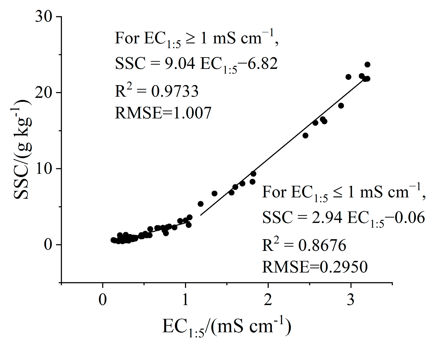
Figure 3.
Spatial distribution of interpolated soil salinity inverted from ECa in the two layers (0–20 cm and 20–60 cm) on different days. Please be notified the inconsistent legend classes used in the two layers over different days.
Figure 3.
Spatial distribution of interpolated soil salinity inverted from ECa in the two layers (0–20 cm and 20–60 cm) on different days. Please be notified the inconsistent legend classes used in the two layers over different days.
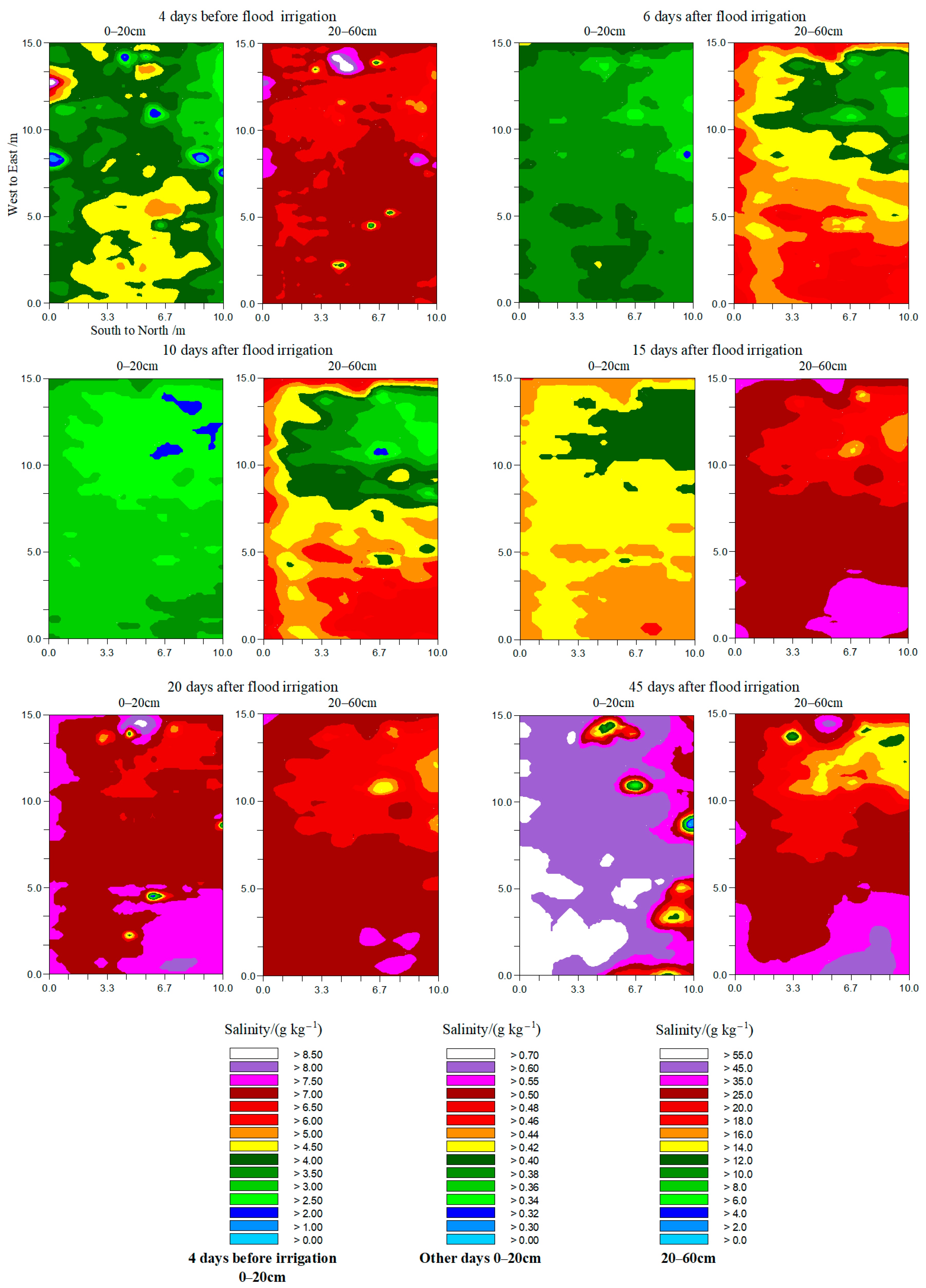
Figure 4.
Temporal variations of soil salt content (SSC) at different layers ((a) 0–20 cm; (b) 20–60 cm) before and after irrigation. B-4, A-6, A-10, A-15, A-20, and A-45, respectively represent 4 days prior to flood irrigation, and 6, 10, 15, 20, and 45 days after flood irrigation.
Figure 4.
Temporal variations of soil salt content (SSC) at different layers ((a) 0–20 cm; (b) 20–60 cm) before and after irrigation. B-4, A-6, A-10, A-15, A-20, and A-45, respectively represent 4 days prior to flood irrigation, and 6, 10, 15, 20, and 45 days after flood irrigation.
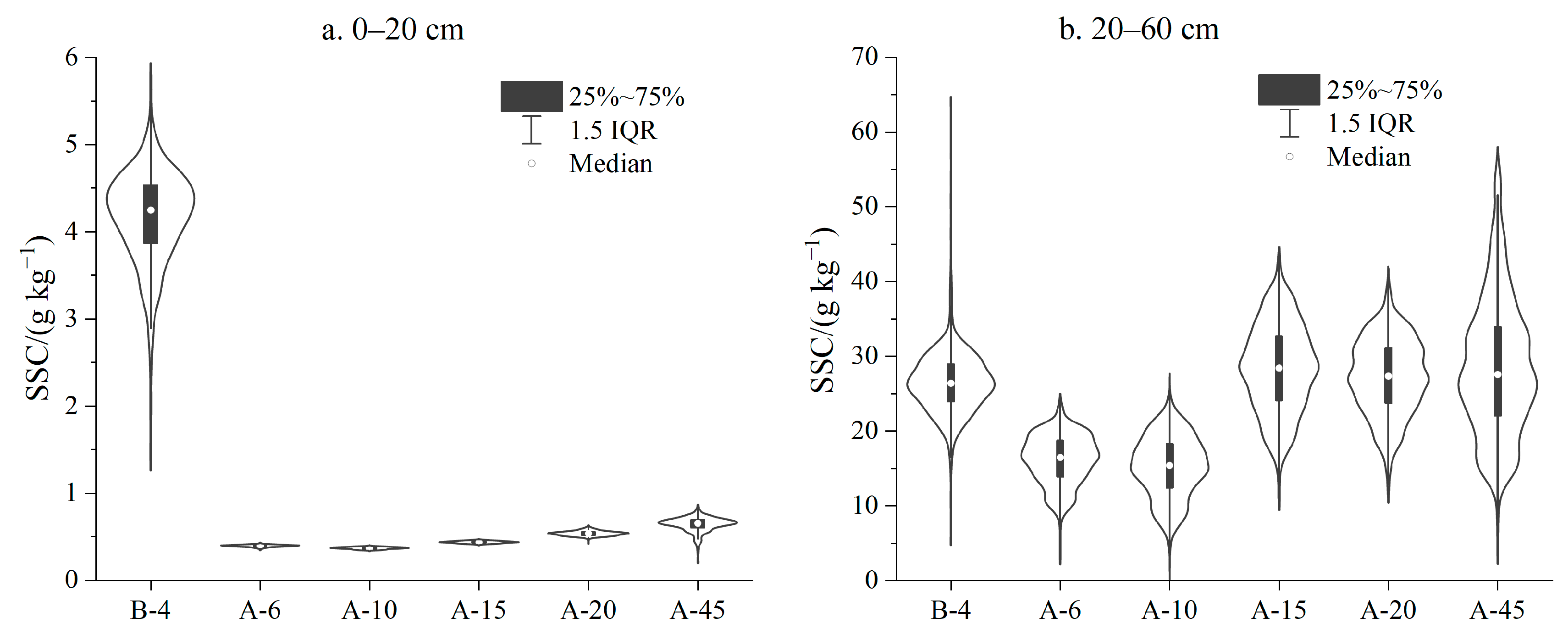
Figure 5.
Correlation of soil salinity between 0–20 cm and 20–60 cm layers on different days before and after irrigation. B-4, A-6, A-10, A-15, A-20, and A-45, respectively represent 4 days prior to flood irrigation, and 6, 10, 15, 20, and 45 days after flood irrigation. Note the unequal ranges of x- and y-axis in different subfigures.

Table 1.
Inversion models between soil salinity and ECa1.0 and ECa0.5 at soil layers on different measurement days.
Table 1.
Inversion models between soil salinity and ECa1.0 and ECa0.5 at soil layers on different measurement days.
| Date | Layer (cm) | Inversion Model | R | Sig. |
|---|---|---|---|---|
| B-4 | 0–20 | SSC = 0.356ECa1.0 − 0.134ECa0.5 − 1.668 | 0.694 | 0.000 |
| 20–60 | SSC = 0.863ECa1.0 + 1.218ECa0.5 − 21.386 | 0.760 | 0.000 | |
| A-6 | 0–20 | SSC = 0.006ECa1.0 − 0.003ECa0.5 + 0.253 | 0.462 | 0.103 |
| 20–60 | SSC = 1.072ECa1.0 − 0.085ECa0.5 − 21.807 | 0.909 | 0.000 | |
| A-10 | 0–20 | SSC = 0.004ECa1.0 + 0.235 | 0.702 | 0.012 |
| 20–60 | SSC = 1.445ECa1.0 − 0.157ECa0.5 − 29.629 | 0.922 | 0.000 | |
| A-15 | 0–20 | SSC = 0.004ECa0.5 + 0.303 | 0.697 | 0.005 |
| 20–60 | SSC = 1.951ECa1.0 − 0.146ECa0.5 − 33.905 | 0.809 | 0.000 | |
| A-20 | 0–20 | SSC = 0.003ECa1.0 + 0.007ECa0.5 + 0.276 | 0.508 | 0.032 |
| 20–60 | SSC = 2.073ECa1.0 − 0.502ECa0.5 − 26.135 | 0.789 | 0.000 | |
| A-45 | 0–20 | SSC = 0.036ECa1.0 − 0.031ECa0.5 + 0.033 | 0.435 | 0.031 |
| 20–60 | SSC = 1.150ECa1.0 + 1.231ECa0.5 − 14.096 | 0.701 | 0.002 |
Note: SSC is soil salinity contents, g kg−1; ECa1.0 and ECa0.5 are soil apparent conductivity corresponding to 1.0 m and 0.5 m coil, respectively, mS cm−1; R is correlation coefficient; B-4, A-6, A-10, A-15, A-20, and A-45, respectively represent 4 days prior to flood irrigation, and 6, 10, 15, 20, and 45 days after flood irrigation. The significance level was p < 0.05.
Table 2.
Best fitting semi-variance models and parameters of soil salinity in two layers on different days.
Table 2.
Best fitting semi-variance models and parameters of soil salinity in two layers on different days.
| Date | Layer (cm) | Model | C0 | C | C0 + C | Range(m) | C0/C0 + C (%) | R2 | RSS |
|---|---|---|---|---|---|---|---|---|---|
| B-4 | 0–20 | Exponential | 0.132 | 0.48 | 0.612 | 18.93 | 21.57 | 0.967 | 0.005 |
| 20–60 | Exponential | 1.550 | 19.91 | 21.46 | 3.51 | 7.22 | 0.967 | 7.8 | |
| A-6 | 0–20 | Spherical | 0.00006 | 0.000204 | 0.000264 | 14.36 | 22.73 | 0.972 | 0.000 |
| 20–60 | Gaussian | 3.19 | 17.47 | 20.66 | 14.62 | 15.44 | 0.984 | 3.54 | |
| A-10 | 0–20 | Spherical | 0.00002 | 0.000278 | 0.0003 | 18.76 | 7.33 | 0.985 | 0.000 |
| 20–60 | Gaussian | 4.05 | 24.04 | 28.09 | 13.04 | 14.42 | 0.984 | 8.95 | |
| A-15 | 0–20 | Spherical | 0.00002 | 0.00031 | 0.000329 | 19.09 | 5.78 | 0.988 | 0.000 |
| 20–60 | Gaussian | 7.50 | 48.5 | 56.00 | 12.64 | 13.39 | 0.985 | 36.4 | |
| A-20 | 0–20 | Exponential | 0.00033 | 0.00097 | 0.0013 | 8.28 | 25.38 | 0.952 | 0.000 |
| 20–60 | Gaussian | 5.50 | 40.83 | 46.33 | 13.94 | 11.87 | 0.988 | 17 | |
| A-45 | 0–20 | Spherical | 0.00193 | 0.00813 | 0.01006 | 12.75 | 19.18 | 0.955 | 0.000 |
| 20–60 | Gaussian | 12.2 | 137 | 149.2 | 15.31 | 8.18 | 0.990 | 124 |
Note: C0 is nugget; C is structure variance; C0 + C is sill; R2 is determination coefficient; RSS is the Residual Sum of Squares; B-4, A-6, A-10, A-15, A-20, and A-45, respectively represent 4 days prior to flood irrigation, and 6, 10, 15, 20, and 45 days after flood irrigation.
Table 3.
Spatial cross-validation of soil salinity in the two layers on different days.
| Date | Layer (cm) | Fitting Model | R2 | SE (g kg−1) | N |
|---|---|---|---|---|---|
| B-4 | 0–20 | y = 0.892x + 0.45 | 0.885 | 0.007 | 3441 |
| 20–60 | y = 0.924x + 2.50 | 0.950 | 0.004 | 3441 | |
| A-6 | 0–20 | y = 0.921x + 0.03 | 0.805 | 0.01 | 3074 |
| 20–60 | y = 0.957x + 0.70 | 0.881 | 0.007 | 3074 | |
| A-10 | 0–20 | y = 0.956x + 0.02 | 0.903 | 0.006 | 3069 |
| 20–60 | y = 0.963x + 0.55 | 0.914 | 0.006 | 3069 | |
| A-15 | 0–20 | y = 0.959x + 0.02 | 0.913 | 0.006 | 3123 |
| 20–60 | y = 0.967x + 0.95 | 0.917 | 0.006 | 3123 | |
| A-20 | 0–20 | y = 0.933x + 0.04 | 0.764 | 0.011 | 3168 |
| 20–60 | y = 0.966x + 0.93 | 0.913 | 0.006 | 3168 | |
| A-45 | 0–20 | y = 0.929x + 0.05 | 0.893 | 0.007 | 3084 |
| 20–60 | y = 0.984x + 0.46 | 0.945 | 0.004 | 3084 |
Note: y is the estimated value of soil salinity content, g kg−1; x is the observed value, g kg−1; R2 is determination coefficient; SE is the standard error, g kg−1; N is the sampling number; B-4, A-6, A-10, A-15, A-20, and A-45, respectively represent 4 days prior to flood irrigation, and 6, 10, 15, 20, and 45 days after flood irrigation.
Table 4.
Classified soil salinity distribution in two soil layers on different days.
| Date | Layer (cm) | Non-Salinized | Slightly Salinized | Moderately Salinized | Heavily Salinized | Saline |
|---|---|---|---|---|---|---|
| (<2 g kg−1) % | (2–4 g kg−1) % | (4–6 g kg−1) % | (6–20 g kg−1) % | (>20 g kg−1) % | ||
| B-4 | 0–20 | 0.05 | 31.60 | 67.91 | 0.45 | 0.00 |
| 20–60 | 0.00 | 0.00 | 0.00 | 3.70 | 96.30 | |
| A-6 | 0–20 | 100.00 | 0.00 | 0.00 | 0.00 | 0.00 |
| 20–60 | 0.00 | 0.00 | 0.00 | 91.17 | 8.83 | |
| A-10 | 0–20 | 100.00 | 0.00 | 0.00 | 0.00 | 0.00 |
| 20–60 | 0.00 | 0.00 | 0.08 | 89.89 | 10.03 | |
| A-15 | 0–20 | 100.00 | 0.00 | 0.00 | 0.00 | 0.00 |
| 20–60 | 0.00 | 0.00 | 0.00 | 8.76 | 91.24 | |
| A-20 | 0–20 | 100.00 | 0.00 | 0.00 | 0.00 | 0.00 |
| 20–60 | 0.00 | 0.00 | 0.00 | 8.27 | 91.73 | |
| A-45 | 0–20 | 100.00 | 0.00 | 0.00 | 0.00 | 0.00 |
| 20–60 | 0.00 | 0.00 | 0.00 | 17.43 | 82.57 |
Note: B-4, A-6, A-10, A-15, A-20, and A-45, respectively represent 4 days prior to flood irrigation, and 6, 10, 15, 20, and 45 days after flood irrigation. Salinization classification was referenced form [35].
Disclaimer/Publisher’s Note: The statements, opinions and data contained in all publications are solely those of the individual author(s) and contributor(s) and not of MDPI and/or the editor(s). MDPI and/or the editor(s) disclaim responsibility for any injury to people or property resulting from any ideas, methods, instructions or products referred to in the content. |
© 2023 by the authors. Licensee MDPI, Basel, Switzerland. This article is an open access article distributed under the terms and conditions of the Creative Commons Attribution (CC BY) license (https://creativecommons.org/licenses/by/4.0/).
Share and Cite
MDPI and ACS Style
He, Y.; Li, X.; Jin, M. Temporal and Spatial Assessment of Soil Salinity Post-Flood Irrigation: A Guide to Optimal Cotton Sowing Timing. Agronomy 2023, 13, 2246. https://doi.org/10.3390/agronomy13092246
AMA Style
He Y, Li X, Jin M. Temporal and Spatial Assessment of Soil Salinity Post-Flood Irrigation: A Guide to Optimal Cotton Sowing Timing. Agronomy. 2023; 13(9):2246. https://doi.org/10.3390/agronomy13092246
Chicago/Turabian StyleHe, Yujiang, Xianwen Li, and Menggui Jin. 2023. "Temporal and Spatial Assessment of Soil Salinity Post-Flood Irrigation: A Guide to Optimal Cotton Sowing Timing" Agronomy 13, no. 9: 2246. https://doi.org/10.3390/agronomy13092246
Note that from the first issue of 2016, this journal uses article numbers instead of page numbers. See further details here.