
Combination of Limited Meteorological Data for Predicting Reference Crop Evapotranspiration Using Artificial Neural Network Method

 ,
,  ,
,  , , , , , ,
Abstract
:1. Introduction
2. Materials and Methods
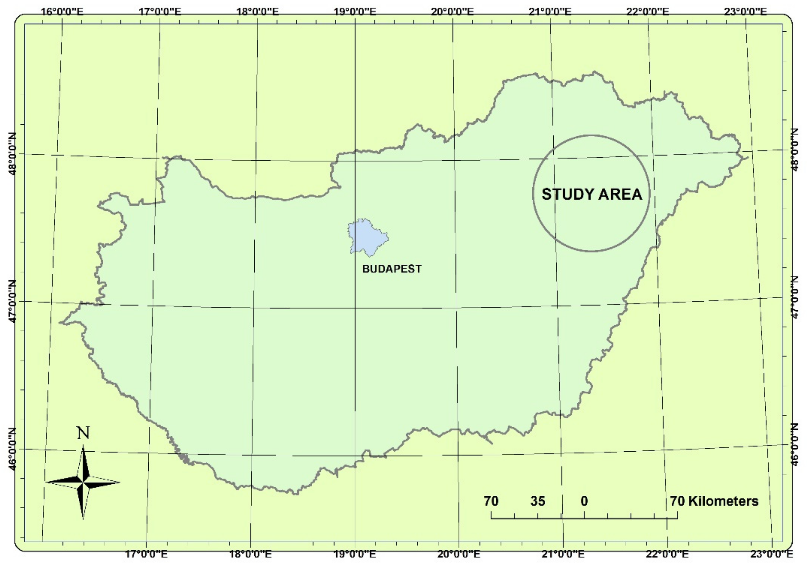
2.1. Study Site
2.2. Data Sources
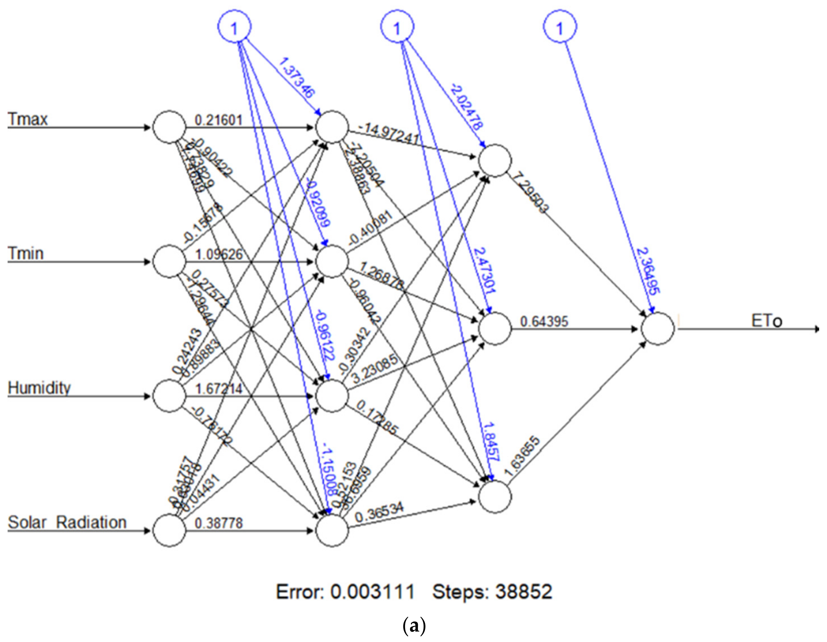
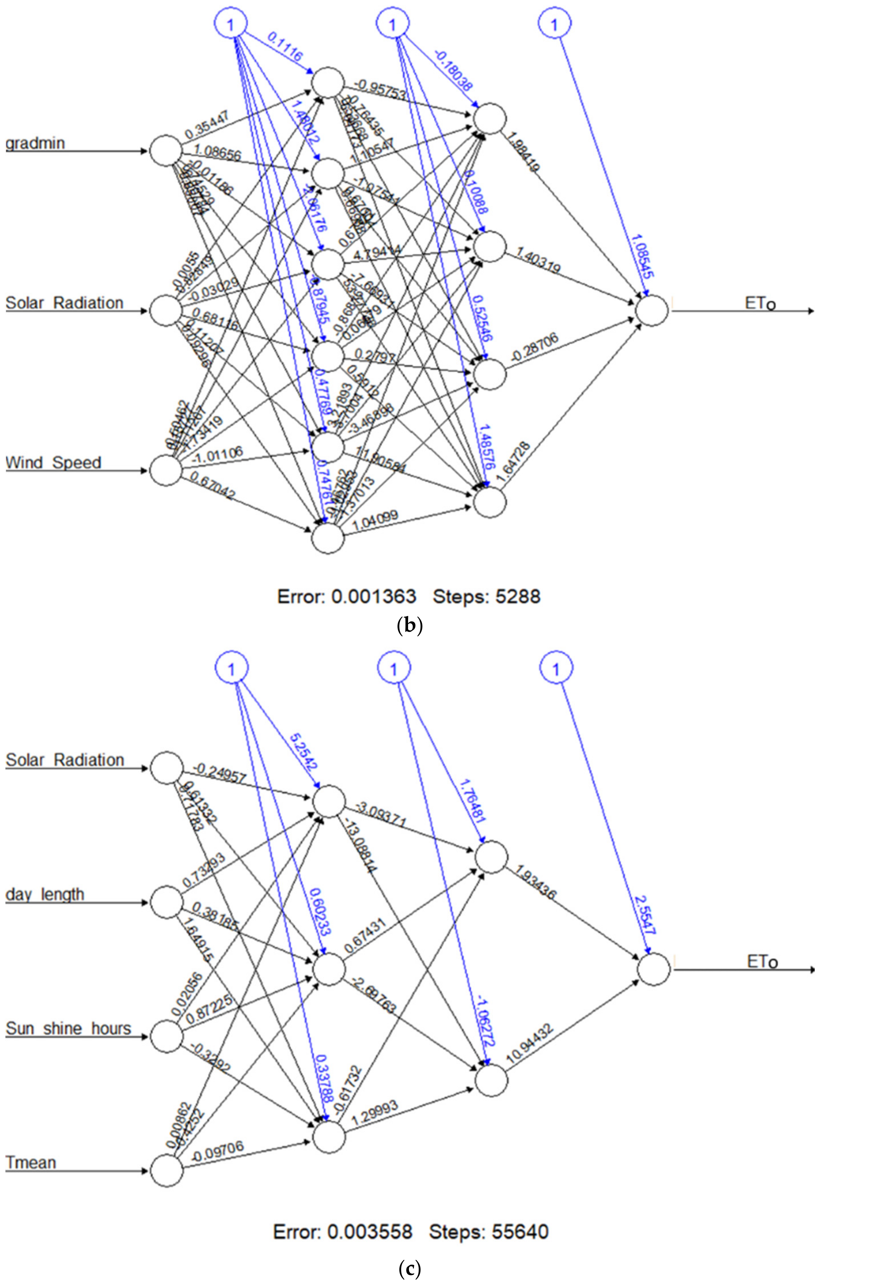
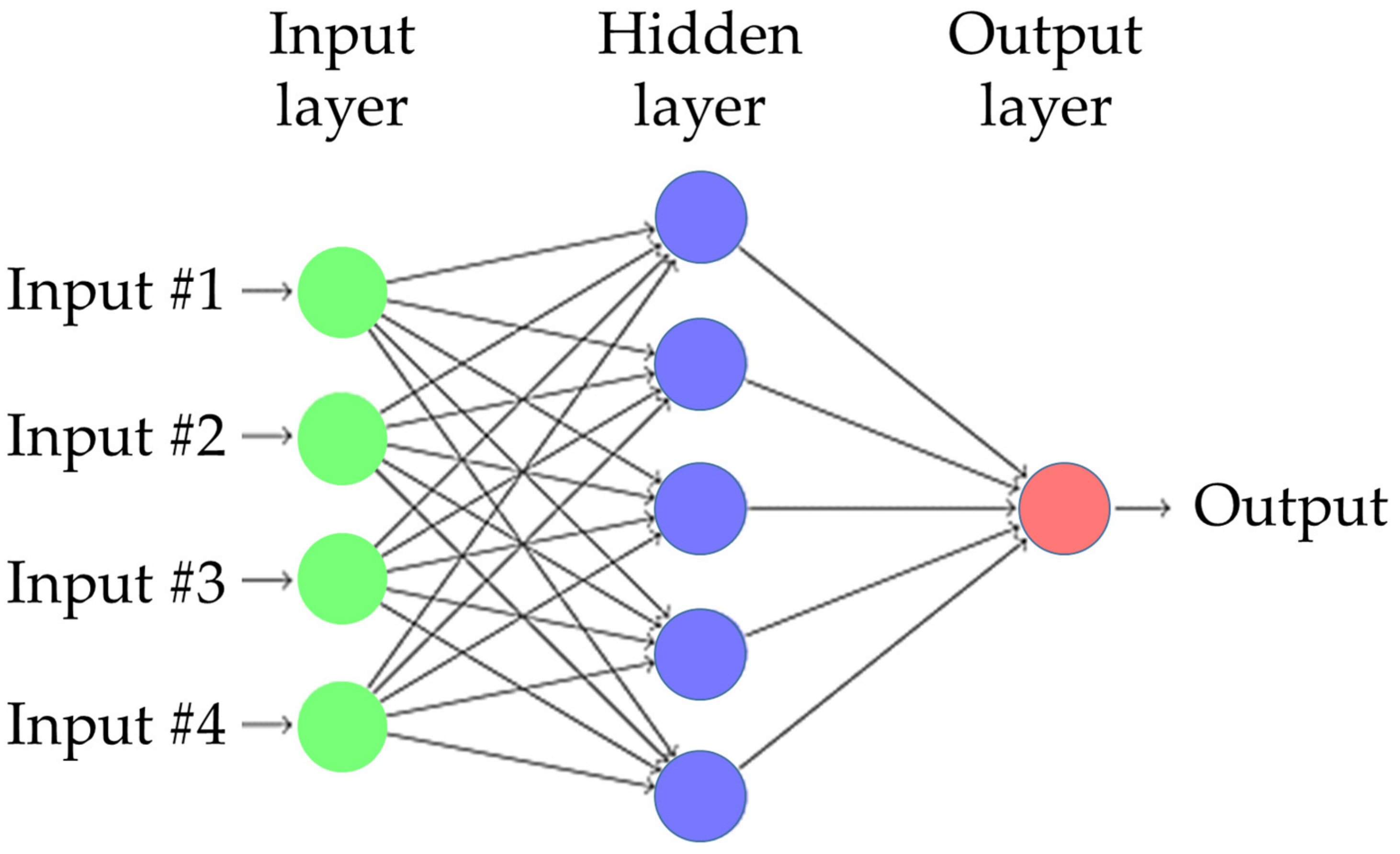
2.3. Application of the Artificial Neural Network method (ANN)
2.4. Performance Evaluation
3. Results
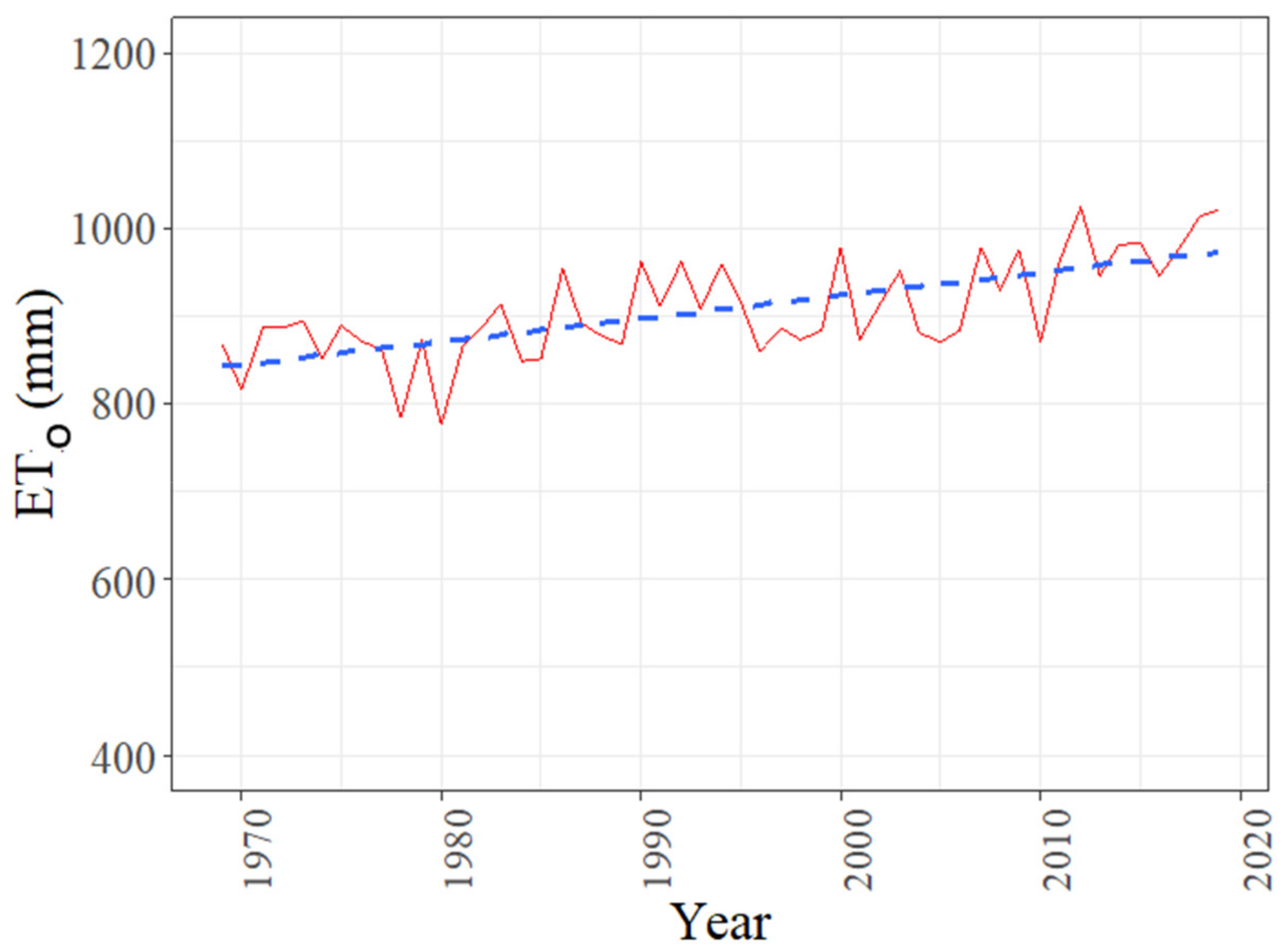
3.1. Calculated ETo
3.2. Data Fusion of Climatic Factors for Modelling the ETo
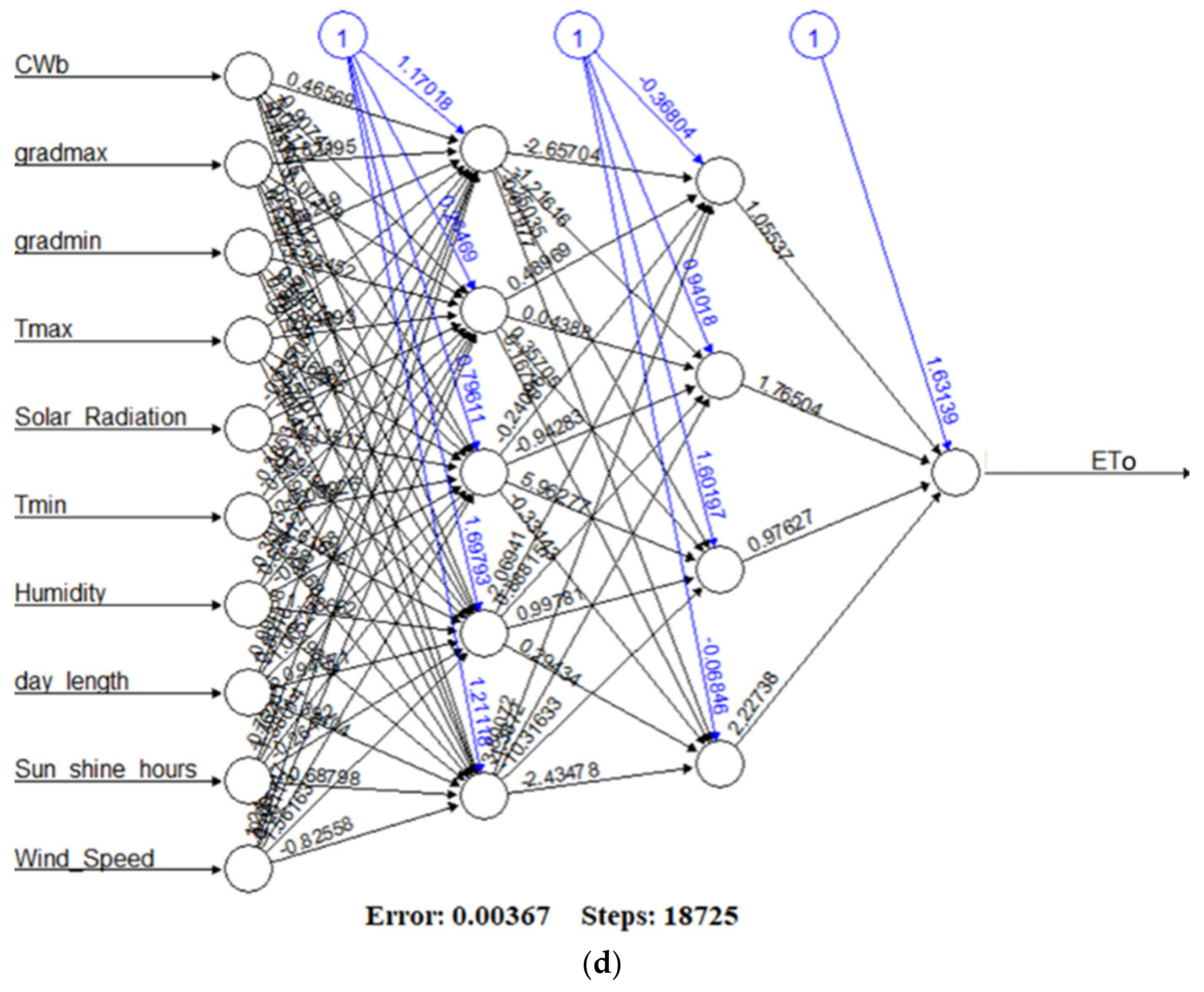
3.3. Structural Network Design of the Superior Models
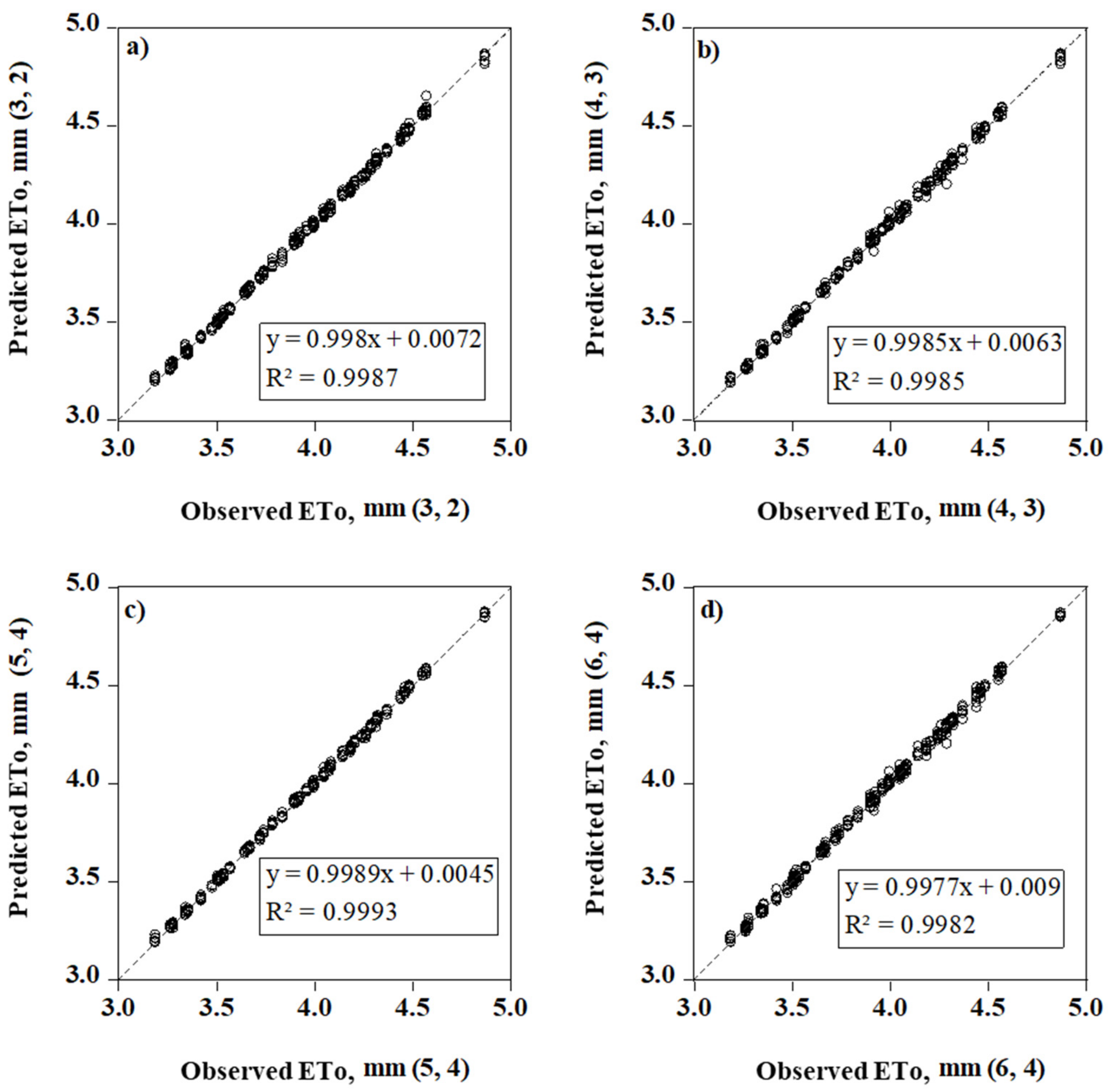
3.4. ETo Prediction and Validation for Superlative ANN Models
4. Discussion
5. Conclusions
Author Contributions
Funding
Data Availability Statement
Acknowledgments
Conflicts of Interest
References
- Bhat, S.A.; Pandit, B.A.; Khan, J.N.; Kumar, R.; Jan, R. Water requirements and irrigation scheduling of maize crop using CROPWAT model. Int. J. Curr. Microbiol. Appl. Sci. 2017, 6, 1662–1670. [Google Scholar] [CrossRef]
- Bhat, S.A.; Pandit, B.; Dar, M.U.D.; Jan, R.; Khan, S.; Mehraj, K. Statistical Comparison of Reference Evapotranspiration Methods: A Case Study from Srinagar in J&K, India. Int. J. Curr. Microbiol. App. Sci. 2017, 6, 3731–3737. [Google Scholar] [CrossRef]
- Elbeltagi, A.; Zhang, L.; Deng, J.; Juma, A.; Wang, K. Modeling monthly crop coefficients of maize based on limited meteorological data: A case study in Nile Delta, Egypt. Comput. Electron. Agric. 2020, 173, 105368. [Google Scholar] [CrossRef]
- Allen, R.G.; Pereira, L.S.; Howell, T.A.; Jensen, M.E. Evapotranspiration information reporting: I. Factors governing measurement accuracy. Agric. Water Manag. 2011, 98, 899–920. [Google Scholar] [CrossRef] [Green Version]
- Allen, R.G.; Pereira, L.S.; Raes, D.; Smith, M. Crop Evapotranspiration-Guidelines for Computing Crop Water Requirements-FAO Irrigation and Drainage Paper 56; FAO: Rome, Italy, 1998; Volume 300, p. D05109. [Google Scholar]
- Elbeltagi, A.; Rizwan, M.; Mokhtar, A.; Deb, P.; Abdullahi, G.; Kushwaha, N.L.; Peroni, L.; Malik, A.; Kumar, N.; Deng, J. Spatial and temporal variability analysis of green and blue evapotranspiration of wheat in the Egyptian Nile Delta from 1997 to 2017. J. Hydrol. 2020, 594, 125662. [Google Scholar] [CrossRef]
- Jerin, J.N.; Islam, H.M.T.; Islam, T.; Shahid, S.; Zhenghua, H.; Mehnaz, B.; Ronghao, C.; Ahmed, E. Spatiotemporal trends in reference evapotranspiration and its driving factors in Bangladesh. Theor. Appl. Climatol. 2021, 144, 793–808. [Google Scholar] [CrossRef]
- Bhat, S.A.; Pandit, B.; Dar, M.U.D.; Rouhullah, S.A.; Jan, R.; Khan, S. Comparative study of different methods of evapotranspiration estimation in Kashmir Valley. J. Agrometeorol. 2017, 19, 383–384. [Google Scholar]
- Mahdi, D.; Sanaz, J.; Samad, E. Climate change impacts on spatial-temporal variations of reference evapotranspiration in Iran. Water Harvest. Res. 2017, 2, 13–23. [Google Scholar] [CrossRef]
- Li, M.; Chu, R.; Shen, S.; Islam, A.R.M.T. Dynamic analysis of pan evaporation variations in the Huai River Basin, a climate transition zone in eastern China. Sci. Total Environ. 2018, 625, 496–509. [Google Scholar] [CrossRef]
- Chu, R.; Li, M.; Islam, A.R.M.T.; Fei, D.; Shen, S. Attribution analysis of actual and potential evapotranspiration changes based on the complementary relationship theory in the Huai River Basin of eastern China. Int. J. Clim. 2019, 39, 4072–4090. [Google Scholar] [CrossRef]
- Pour, S.H.; Wahab, A.K.A.; Shahid, S.; Ismail, Z.B. Changes in reference evapotranspiration and its driving factors in peninsular Malaysia. Atmos. Res. 2020, 246, 105096. [Google Scholar] [CrossRef]
- Guo, D.; Westra, S.; Maier, H.R. Sensitivity of potential evapotranspiration to changes in climate variables for different Australian climatic zones. Hydrol. Earth Syst. Sci. 2017, 21, 2107–2126. [Google Scholar] [CrossRef] [Green Version]
- Pan, S.; Tian, H.; Dangal, S.R.S.; Yang, Q.; Yang, J.; Lu, C.; Tao, B.; Ren, W.; Ouyang, Z. Responses of global terrestrial evapotranspiration to climate change and increasing atmospheric CO2 in the 21st century. Earth’s Future 2015, 3, 15–35. [Google Scholar] [CrossRef]
- Wang, W.; Li, C.; Xing, W.; Fu, J. Projecting the potential evapotranspiration by coupling different formulations and input data reliabilities: The possible uncertainty source for climate change impacts on hydrological regime. J. Hydrol. 2017, 555, 298–313. [Google Scholar] [CrossRef]
- Lu, Y.; Ma, D.; Chen, X.; Zhang, J. A simple method for estimating field crop evapotranspiration from pot experiments. Water 2018, 10, 1823. [Google Scholar] [CrossRef] [Green Version]
- Ünlü, M.; Kanber, R.; Kapur, B. Comparison of soybean evapotranspirations measured by weighing lysimeter and Bowen ratio-energy balance methods. Afr. J. Biotechnol. 2010, 9, 4700–4713. [Google Scholar] [CrossRef]
- Başağaoğlu, H.; Chakraborty, D.; Winterle, J. Reliable evapotranspiration predictions with a probabilistic machine learning framework. Water 2021, 13, 557. [Google Scholar] [CrossRef]
- Dimitriadou, S.; Nikolakopoulos, K.G. Reference Evapotranspiration (ETo) Methods Implemented as ArcMap Models with Remote-Sensed and Ground-Based Inputs, Examined along with MODIS ET, for Peloponnese, Greece. ISPRS Int. J. Geo-Inf. 2021, 10, 390. [Google Scholar] [CrossRef]
- Milly, P.C.D.; Dunne, K.A. Potential evapotranspiration and continental drying. Nat. Clim. Chang. 2016, 6, 946–949. [Google Scholar] [CrossRef]
- Wang, H.; Li, X.; Tan, J. Interannual variations of evapotranspiration and water use efficiency over an oasis cropland in arid regions of North-Western China. Water 2020, 12, 1239. [Google Scholar] [CrossRef]
- McMahon, T.A.; Peel, M.C.; Lowe, L.; Srikanthan, R.; McVicar, T.R. Estimating actual, potential, reference crop and pan evaporation using standard meteorological data: A pragmatic synthesis. Hydrol. Earth Syst. Sci. 2013, 17, 1331–1363. [Google Scholar] [CrossRef] [Green Version]
- Bai, P.; Liu, X.; Yang, T.; Li, F.; Liang, K.; Hu, S.; Liu, C. Assessment of the influences of different potential evapotranspiration inputs on the performance of monthly hydrological models under different climatic conditions. J. Hydrometeorol. 2016, 17, 2259–2274. [Google Scholar] [CrossRef]
- Zhao, L.; Xia, J.; Xu, C.; Wang, Z.; Sobkowiak, L.; Long, C. Evapotranspiration estimation methods in hydrological models. J. Geogr. Sci. 2013, 23, 359–369. [Google Scholar] [CrossRef]
- Jing, W.; Yaseen, Z.M.; Shahid, S.; Saggi, M.K.; Tao, H.; Kisi, O.; Salih, S.Q.; Al-Ansari, N.; Chau, K.W. Implementation of evolutionary computing models for reference evapotranspiration modeling: Short review, assessment and possible future research directions. Eng. Appl. Comput. Fluid Mech. 2019, 13, 811–823. [Google Scholar] [CrossRef] [Green Version]
- Ren, X.; Qu, Z.; Martins, D.S.; Paredes, P.; Pereira, L.S. Daily reference evapotranspiration for hyper-arid to moist sub-humid climates in inner mongolia, China: I. Assessing temperature methods and spatial variability. Water Resour. Manag. 2016, 30, 3769–3791. [Google Scholar] [CrossRef]
- Kisi, O.; Shiri, J.; Karimi, S.; Adnan, R.M. Three different adaptive neuro fuzzy computing techniques for forecasting long-period daily streamflows. In Big Data in Engineering Applications; Roy, S.S., Samui, P., Deo, R., Ntalampiras, S., Eds.; Springer: Singapore, 2018; pp. 303–321. [Google Scholar]
- Khosravinia, P.; Nikpour, M.R.; Kisi, O.; Yaseen, Z.M. Application of novel data mining algorithms in prediction of discharge and end depth in trapezoidal sections. Comput. Electron. Agric. 2020, 170, 105283. [Google Scholar] [CrossRef]
- Torres, A.F.; Walker, W.R.; McKee, M. Forecasting daily potential evapotranspiration using machine learning and limited climatic data. Agric. Water Manag. 2011, 98, 553–562. [Google Scholar] [CrossRef]
- Mehdizadeh, S. Estimation of daily reference evapotranspiration (ETo) using artificial intelligence methods: Offering a new approach for lagged ETo data-based modeling. J. Hydrol. 2018, 559, 794–812. [Google Scholar] [CrossRef]
- Gorka, L.; Amais, O.B.; Jose, J.L. Comparison of artificial neural network models and empirical and semi-empirical equations for daily reference evapotranspiration estimation in the Basque Country (Northern Spain). Agric. Water Manag. 2008, 95, 553–565. [Google Scholar] [CrossRef]
- Haykin, S. Neural Networks. A Comprehensive Foundation; Prentice Hall International Inc.: Hoboken, NJ, USA, 1999; p. 823. [Google Scholar]
- Alizamir, M.; Kisi, O.; Muhammad Adnan, R.; Kuriqi, A. Modelling reference evapotranspiration by combining neuro-fuzzy and evolutionary strategies. Acta Geophys. 2020, 68, 1113–1126. [Google Scholar] [CrossRef]
- Zhu, B.; Feng, Y.; Gong, D.; Jiang, S.; Zhao, L.; Cui, N. Hybrid particle swarm optimization with extreme learning machine for daily reference evapotranspiration prediction from limited climatic data. Comput. Electron. Agric. 2020, 173, 105430. [Google Scholar] [CrossRef]
- Elragal, H.M. Improving neural networks prediction accuracy using particle swarm optimization combiner. Int. J. Neural Syst. 2009, 19, 387–393. [Google Scholar] [CrossRef] [PubMed]
- Pidaparti, R.M.; Jayanti, S.; Palakal, M.J. Residual Strength and Corrosion Rate Predictions of Aging Aircraft Panels: Neural Network Study. J. Aircr. 2002, 39, 175–180. [Google Scholar] [CrossRef]
- Pidaparti, R. Aircraft structural integrity assessment through computational intelligence techniques. Struct. Durab. Health Monit. 2006, 2, 131–148. [Google Scholar] [CrossRef]
- Hijazi, A.; Al-Dahidi, S.; Altarazi, S. Residual Strength Prediction of Aluminum Panels with Multiple Site Damage Using Artificial Neural Networks. Materials 2020, 13, 5216. [Google Scholar] [CrossRef]
- Ince, R. Prediction of fracture parameters of concrete by Artificial Neural Networks. Eng. Fract. Mech. 2004, 71, 2143–2159. [Google Scholar] [CrossRef]
- De, S.; Debnath, A. Artificial neural network based prediction of maximum and minimum temperature in the summer monsoon months over India. Appl. Phys. Res. 2009, 1, 37. [Google Scholar] [CrossRef] [Green Version]
- Malik, H.; Singh, S. Application of artificial neural network for long term wind speed prediction. In Proceedings of the Conference on Advances in Signal Processing (CASP), Pune, India, 9–11 June 2016; Institute of Electrical and Electronics Engineers: New Jersey, NJ, USA, 2016; pp. 217–222. [Google Scholar] [CrossRef]
- Adisa, O.M.; Botai, J.O.; Adeola, A.M.; Hassen, A.; Botai, C.M.; Darkey, D.; Tesfamariam, E. Application of artificial neural network for predicting maize production in South Africa. Sustainability 2019, 11, 1145. [Google Scholar] [CrossRef] [Green Version]
- Moghaddam, M.G.; Ahmad, F.B.H.; Basri, M.; Rahman, M.B.A. Artificial neural network modeling studies to predict the yield of enzymatic synthesis of betulinic acid ester. Electron. J. Biotechnol. 2010, 13, 3–4. [Google Scholar] [CrossRef]
- Nema, M.K.; Khare, D.; Chandniha, S.K. Application of artificial intelligence to estimate the reference evapotranspiration in sub-humid Doon valley. Appl. Water Sci. 2017, 7, 3903–3910. [Google Scholar] [CrossRef] [Green Version]
- Adnan, R.M.; Chen, Z.; Yuan, X.; Kisi, O.; El-Shafie, A.; Kuriqi, A.; Ikram, M. Reference Evapotranspiration Modeling Using New Heuristic Methods. Entropy 2020, 22, 547. [Google Scholar] [CrossRef] [PubMed]
- Yin, Z.; Wen, X.; Feng, Q.; He, Z.; Zou, S.; Yang, L. Integrating genetic algorithm and support vector machine for modeling daily reference evapotranspiration in a semi-arid mountain area. Hydrol. Res. 2016, 48, 1177–1191. [Google Scholar] [CrossRef]
- Jovic, S.; Nedeljkovic, B.; Golubovic, Z.; Kostic, N. Evolutionary algorithm for reference evapotranspiration analysis. Comput. Electron. Agric. 2018, 150, 1–4. [Google Scholar] [CrossRef]
- Mohammed, S.; Alsafadi, K.; Daher, H.; Gombos, B.; Mahmood, S.; Harsányi, E. Precipitation pattern changes and response of vegetation to drought variability in the eastern Hungary. Bull. Natl. Res. Cent. 2020, 44, 55. [Google Scholar] [CrossRef] [Green Version]
- Takács, I.; Amiri, M.; Károly, K.; Mohammed, S. Assessing soil quality changes after 10 years of agricultural activities in eastern Hungary. Irrig. Drain. 2021, 70, 1116–1128. [Google Scholar] [CrossRef]
- Mohammed, S.; Mirzaei, M.; Pappné Törő, Á.; Anari, M.G.; Moghiseh, E.; Asadi, H.; Harsányi, E. Soil carbon dioxide emissions from maize (Zea mays L.) fields as influenced by tillage management and climate. Irrig. Drain. 2021, 71, 228–240. [Google Scholar] [CrossRef]
- Keskin, T.E.; Düğenci, M.; Kaçaroğlu, F. Prediction of water pollution sources using artificial neural networks in the study areas of Sivas, Karabuk and Bartın (Turkey). Environ. Earth Sci. 2015, 73, 5333–5347. [Google Scholar] [CrossRef]
- Elbeltagi, A.; Deng, J.; Wang, K.; Hong, Y. Crop Water footprint estimation and modeling using an arti fi cial neural network approach in the Nile Delta, Egypt. Agric. Water Manag. 2020, 235, 106080. [Google Scholar] [CrossRef]
- Elbeltagi, A.; Deng, J.; Wang, K.; Malik, A.; Maroufpoor, S. Modeling long-term dynamics of crop evapotranspiration using deep learning in a semi-arid environment. Agric. Water Manag. 2020, 241, 106334. [Google Scholar] [CrossRef]
- Juhász, C.; Gálya, B.; Kovács, E.; Nagy, A.; Tamás, J.; Huzsvai, L. Seasonal predictability of weather and crop yield in regions of Central European continental climate. Comput. Electron. Agric. 2020, 173, 105400. [Google Scholar] [CrossRef]
- Celik, S. The effects of climate change on human behaviors. In Environment, Climate, Plant and Vegetation Growth; Fahad, S., Hasanuzzaman, M., Alam, M., Ullah, H., Saeed, M., Khan, I.A., Adnan, M., Eds.; Springer: Cham, Switzerland, 2020; pp. 577–589. [Google Scholar]
- Mupedziswa, R.; Kubanga, K.P. Climate change, urban settlements and quality of life: The case of the Southern African Development Community region. Dev. S. Afr. 2017, 34, 196–209. [Google Scholar] [CrossRef]
- Pecl, G.T.; Araújo, M.B.; Bell, J.D.; Blanchard, J.; Bonebrake, T.C.; Chen, I.C.; Williams, S.E. Biodiversity redistribution under climate change: Impacts on ecosystems and human well-being. Science 2017, 355, eaai9214. [Google Scholar] [CrossRef] [PubMed]
- Cane, M.A.; Clement, A.C.; Kaplan, A.; Kushnir, Y.; Pozdnyakov, D.; Seager, R.; Murtugudde, R. Twentieth-century sea surface temperature trends. Science 1997, 275, 957–960. [Google Scholar] [CrossRef] [PubMed] [Green Version]
- Maček, U.; Bezak, N.; Šraj, M. Reference evapotranspiration changes in Slovenia, Europe. Agric. For. Meteorol. 2018, 260, 183–192. [Google Scholar] [CrossRef]
- Hari, V.; Rakovec, O.; Markonis, Y.; Hanel, M.; Kumar, R. Increased future occurrences of the exceptional 2018–2019 Central European drought under global warming. Sci. Rep. 2020, 10, 12207. [Google Scholar] [CrossRef] [PubMed]
- Hassan, W.H.; Nile, B.K. Climate change and predicting future temperature in Iraq using CanESM2 and HadCM3 modeling. Modeling Earth Syst. Environ. 2021, 7, 737–748. [Google Scholar] [CrossRef]
- McVicar, T.R.; Roderick, M.L.; Donohue, R.J.; Li, L.T.; Van Niel, T.G.; Thomas, A.; Dinpashoh, Y. Global review and synthesis of trends in observed terrestrial near-surface wind speeds: Implications for evaporation. J. Hydrol. 2012, 416, 182–205. [Google Scholar] [CrossRef]
- Wang, H.; Rogers, J.C.; Munroe, D.K. Commonly used drought indices as indicators of soil moisture in China. J. Hydrometeorol. 2015, 16, 1397–1408. [Google Scholar] [CrossRef]
- Sheffield, J.; Goteti, G.; Wen, F.; Wood, E.F. A simulated soil moisture based drought analysis for the United States. J. Geophys. Res. Atmos. 2004, 109, D24108. [Google Scholar] [CrossRef]
- Alsafadi, K.; Mohammed, S.; Ayugi, B.; Sharaf, M.; Harsányi, E. Spatial–temporal evolution of drought characteristics over Hungary between 1961 and 2010. Pure Appl. Geophys. 2020, 177, 3961–3978. [Google Scholar] [CrossRef] [Green Version]
- Matyasovszky, I.; Weidinger, T.; Bartholy, J.; Barcza, Z. Current regional climate 652 change studies in Hungary: A review. Geogr. Helv. 1999, 54, 138–146, 653. [Google Scholar] [CrossRef] [Green Version]
- Lockwood, M.; Owens, M.; Barnard, L.; Davis, C.; Thomas, S. Solar cycle 24: What is the Sun up to? Astron. Geophys. 2012, 53, 3.9–3.15. [Google Scholar] [CrossRef] [Green Version]
- Mares, I.; Dobrica, V.; Mares, C.; Demetrescu, C. Assessing the solar variability signature in climate variables by information theory and wavelet coherence. Sci. Rep. 2021, 11, 11337. [Google Scholar] [CrossRef] [PubMed]
- Bakucs, Z.; Fertő, I.; Vígh, E. Crop Productivity and Climatic Conditions: Evidence from Hungary. Agriculture 2020, 10, 421. [Google Scholar] [CrossRef]
- Nagy, A.; Tamás, J. Integrated airborne and field methods to characterize soil water regime. In Peer-Reviewed Contributions, Transport of Water, Chemicals and Energy in the Soil-Plant-Atmosphere System; Celkova, A., Ed.; Institute of Hydrology, Slovak Academy of Sciences: Bratislava, Slovakia, 2009; pp. 412–420. [Google Scholar]
- Szalmáné Csete, M.; Buzási, A. Hungarian regions and cities towards an adaptive future-analysis of climate change strategies on different spatial levels. Időjárás/Q. J. Hung. Meteorol. Serv. 2020, 124, 253–276. [Google Scholar] [CrossRef]
- Tamás, J.; Nagy, A.; Fehér, J. Agricultural biomass monitoring on watersheds based on remote sensed data. Water Sci. Technol. 2015, 72, 2212–2220. [Google Scholar] [CrossRef]


| Combinations | Variables | Hidden Neuron | RMSE (mm) | MAPE (%) | NRMSE (%) | ACC (%) | R2 |
|---|---|---|---|---|---|---|---|
| C1 | Tmean + Sunshine hours + CWB | 5, 4 | 0.071 | 0.005 | 0.032 | 0.995 | 0.98 |
| 4, 3 | 0.140 | 0.020 | 0.123 | 0.990 | 0.95 | ||
| 3, 2 | 0.257 | 0.072 | 0.425 | 0.986 | 0.85 | ||
| 6, 4 | 0.119 | 0.013 | 0.102 | 0.991 | 0.96 | ||
| 4, 2 | 0.159 | 0.025 | 0.281 | 0.997 | 0.94 | ||
| C2 | Tmax + Tmin + Humidity + Solar Radiation | 5, 4 | 0.011 | 0.0006 | 0.001 | 0.998 | 0.99 |
| 4, 3 | 0.008 | 0.0000 | 0.000 | 0.999 | 0.99 | ||
| 3, 2 | 0.012 | 0.0003 | 0.001 | 0.998 | 0.99 | ||
| 6, 4 | 0.015 | 0.0011 | 0.001 | 0.998 | 0.99 | ||
| 4, 2 | 0.019 | 0.0014 | 0.003 | 0.999 | 0.99 | ||
| C3 | Gradmax + Sunshine hours + Windspeed | 5, 4 | 0.549 | 0.316 | 1.945 | 0.996 | 0.31 |
| 4, 3 | 0.548 | 0.315 | 1.943 | 0.994 | 0.30 | ||
| 3, 2 | 0.548 | 0.318 | 2.038 | 0.995 | 0.31 | ||
| 6, 4 | 0.549 | 0.316 | 1.979 | 0.996 | 0.30 | ||
| 4, 2 | 0.548 | 0.315 | 1.976 | 0.996 | 0.31 | ||
| C4 | Gradmin + Solar Radiation + Windspeed | 5, 4 | 0.013 | 0.000 | 0.001 | 0.996 | 0.99 |
| 4, 3 | 0.011 | 0.000 | 0.001 | 0.999 | 0.99 | ||
| 3, 2 | 0.027 | 0.004 | 0.005 | 0.998 | 0.99 | ||
| 6, 4 | 0.010 | 0.000 | 0.001 | 0.999 | 0.99 | ||
| 4, 2 | 0.017 | 0.003 | 0.001 | 0.99 | 0.99 | ||
| C5 | CWB + Humidity + Windspeed | 5, 4 | 0.432 | 0.194 | 0.855 | 0.998 | 0.57 |
| 4, 3 | 0.433 | 0.193 | 0.701 | 0.998 | 0.57 | ||
| 3, 2 | 0.435 | 0.195 | 0.887 | 0.998 | 0.56 | ||
| 6, 4 | 0.427 | 0.187 | 0.879 | 0.998 | 0.57 | ||
| 4, 2 | 0.435 | 0.194 | 0.835 | 0.998 | 0.56 | ||
| C6 | Sunshine hours + Tmax + day length | 5, 4 | 0.155 | 0.022 | 0.087 | 0.997 | 0.94 |
| 4, 3 | 0.179 | 0.030 | 0.128 | 0.998 | 0.92 | ||
| 3, 2 | 0.372 | 0.140 | 0.690 | 0.994 | 0.68 | ||
| 6, 4 | 0.206 | 0.041 | 0.168 | 0.993 | 0.90 | ||
| 4, 2 | 0.371 | 0.140 | 0.552 | 0.998 | 0.68 | ||
| C7 | Solar Radiation + day length + Sunshine hours + Tmean | 5, 4 | 0.0234 | 0.0025 | 0.003 | 0.998 | 0.99 |
| 4, 3 | 0.0165 | 0.0012 | 0.001 | 0.999 | 0.99 | ||
| 3, 2 | 0.0147 | 0.0003 | 0.001 | 0.999 | 0.99 | ||
| 6, 4 | 0.0345 | 0.0007 | 0.004 | 0.997 | 0.99 | ||
| 4, 2 | 0.0307 | 0.0012 | 0.004 | 0.998 | 0.99 | ||
| C8 | CWB + Gradmax + Gradmin + Tmax + Solar Radiation + Tmin + Humidity + day length + Sunshine hours + Windspeed | 5, 4 | 0.0170 | 0.0006 | 0.001 | 0.999 | 0.99 |
| 4, 3 | 0.0282 | 0.0008 | 0.003 | 0.999 | 0.99 | ||
| 3, 2 | 0.0330 | 0.0006 | 0.004 | 0.999 | 0.99 | ||
| 6, 4 | 0.0204 | 0.0017 | 0.002 | 0.999 | 0.99 | ||
| 4, 2 | 0.0232 | 0.0019 | 0.003 | 0.999 | 0.99 |
| Combinations | Hidden Neuron | RMSE (mm) | MAPE (%) | NRMSE (%) | ACC (%) | R2 |
|---|---|---|---|---|---|---|
| C1 | 5, 4 | 0.071 | 0.005 | 0.032 | 0.995 | 0.98 |
| C2 | 4, 3 | 0.008 | 0.0000 | 0.000 | 0.999 | 0.99 |
| C3 | 4, 2 | 0.548 | 0.315 | 1.976 | 0.996 | 0.31 |
| C4 | 6, 4 | 0.010 | 0.000 | 0.001 | 0.999 | 0.99 |
| C5 | 6, 4 | 0.427 | 0.187 | 0.879 | 0.998 | 0.57 |
| C6 | 6, 4 | 0.206 | 0.041 | 0.168 | 0.993 | 0.90 |
| C7 | 3, 2 | 0.0147 | 0.0003 | 0.001 | 0.999 | 0.99 |
| C8 | 5, 4 | 0.017 | 0.0006 | 0.001 | 0.999 | 0.99 |
Publisher’s Note: MDPI stays neutral with regard to jurisdictional claims in published maps and institutional affiliations. |
© 2022 by the authors. Licensee MDPI, Basel, Switzerland. This article is an open access article distributed under the terms and conditions of the Creative Commons Attribution (CC BY) license (https://creativecommons.org/licenses/by/4.0/).
Share and Cite
Elbeltagi, A.; Nagy, A.; Mohammed, S.; Pande, C.B.; Kumar, M.; Bhat, S.A.; Zsembeli, J.; Huzsvai, L.; Tamás, J.; Kovács, E.; et al. Combination of Limited Meteorological Data for Predicting Reference Crop Evapotranspiration Using Artificial Neural Network Method. Agronomy 2022, 12, 516. https://doi.org/10.3390/agronomy12020516
Elbeltagi A, Nagy A, Mohammed S, Pande CB, Kumar M, Bhat SA, Zsembeli J, Huzsvai L, Tamás J, Kovács E, et al. Combination of Limited Meteorological Data for Predicting Reference Crop Evapotranspiration Using Artificial Neural Network Method. Agronomy. 2022; 12(2):516. https://doi.org/10.3390/agronomy12020516
Chicago/Turabian StyleElbeltagi, Ahmed, Attila Nagy, Safwan Mohammed, Chaitanya B. Pande, Manish Kumar, Shakeel Ahmad Bhat, József Zsembeli, László Huzsvai, János Tamás, Elza Kovács, and et al. 2022. "Combination of Limited Meteorological Data for Predicting Reference Crop Evapotranspiration Using Artificial Neural Network Method" Agronomy 12, no. 2: 516. https://doi.org/10.3390/agronomy12020516