Article

Simultaneous Calibration of Grapevine Phenology and Yield with a Soil–Plant–Atmosphere System Model Using the Frequentist Method

1
Centre for the Research and Technology of Agro-Environmental and Biological Sciences (CITAB), Institute for Innovation, Capacity Building and Sustainability of Agri-Food Production (Inov4Agro), University of Trás-os-Montes and Alto Douro (UTAD), 5000-801 Vila Real, Portugal
2
Potsdam Institute for Climate Impact Research, PIK, 14473 Potsdam, Germany
3
CoLAB VINES & WINES-National Collaborative Laboratory for the Portuguese Wine Sector, Associação para o Desenvolvimento da Viticultura Duriense (ADVID), Edifício Centro de Excelência da Vinha e do Vinho, Régia Douro Park, 5000-033 Vila Real, Portugal
*
Author to whom correspondence should be addressed.
Agronomy 2021, 11(8), 1659; https://doi.org/10.3390/agronomy11081659
Submission received: 8 July 2021 / Revised: 12 August 2021 / Accepted: 18 August 2021 / Published: 20 August 2021
(This article belongs to the Special Issue Predictive Modeling to Aid Agronomic Decision Making)

Abstract

:
Reliable estimations of parameter values and associated uncertainties are crucial for crop model applications in agro-environmental research. However, estimating many parameters simultaneously for different types of response variables is difficult. This becomes more complicated for grapevines with different phenotypes between varieties and training systems. Our study aims to evaluate how a standard least square approach can be used to calibrate a complex grapevine model for simulating both the phenology (flowering and harvest date) and yield of four different variety–training systems in the Douro Demarcated Region, northern Portugal. An objective function is defined to search for the best-fit parameters that result in the minimum value of the unweighted sum of the normalized Root Mean Squared Error (nRMSE) of the studied variables. Parameter uncertainties are estimated as how a given parameter value can determine the total prediction variability caused by variations in the other parameter combinations. The results indicate that the best-estimated parameters show a satisfactory predictive performance, with a mean bias of −2 to 4 days for phenology and −232 to 159 kg/ha for yield. The corresponding variance in the observed data was generally well reproduced, except for one occasion. These parameters are a good trade-off to achieve results close to the best possible fit of each response variable. No parameter combinations can achieve minimum errors simultaneously for phenology and yield, where the best fit to one variable can lead to a poor fit to another. The proposed parameter uncertainty analysis is particularly useful to select the best-fit parameter values when several choices with equal performance occur. A global sensitivity analysis is applied where the fruit-setting parameters are identified as key determinants for yield simulations. Overall, the approach (including uncertainty analysis) is relatively simple and straightforward without specific pre-conditions (e.g., model continuity), which can be easily applied for other models and crops. However, a challenge has been identified, which is associated with the appropriate assumption of the model errors, where a combination of various calibration approaches might be essential to have a more robust parameter estimation.

Graphical Abstract

1. Introduction

Process-based crop models have been frequently applied to simulate climate change impacts and the potential adaptation options of the cropping system [1,2,3]. They are important tools to support agricultural policy development in anticipation of global climate change. However, crop models have also been identified as an important source of uncertainties in projecting climate impacts, which may hinder robust projections and the identification of cause–effect relationships [3,4]. It is thus important to quantify, manage and reduce these uncertainties to improve the reliability of impact projections and better evaluate potential adaptation measures. One of the most important approaches, to considerably reduce the uncertainties, is through adequate model calibration [1,4]. Climate impact modelling studies should pay particular attention to how the model is calibrated, as the projected impacts can be significantly different when the model is differently calibrated [2,4,5].
Crop models are typically composed of various mathematical equations that are mainly derived from field experimentations to describe crop development and growth, taking into account complex interactions among genotype, management and environment [2]. The application of models to different environments often requires model calibration, by which some model parameters are adjusted to reflect the local conditions in order to adequately address a relevant research issue [6]. However, the estimated parameter values are largely affected by the approach used for the calibration. There is a large diversity of calibration approaches, with different approaches having their own calibration steps and statistical model of errors, thus resulting in different parameter values given the same data [5,7,8]. The fundamental choice in employing a calibration approach depends on whether we consider the simulated values as random variables or not [9,10,11]. A random assumption explicitly considers uncertainties in the predictors, namely, the model structure, parameters and input variables, and thereby their random variability becomes an important source of errors [9]. The random approach allows quantifying a specific source of uncertainty, e.g., estimate the contributions of the model structure and parameter uncertainties to the total prediction uncertainties [10]. Nonetheless, there are difficulties in estimating the plausible prior distribution of the model structures, parameter vectors and all relevant inputs, from which the appropriate sample sizes are drawn [10,11]. Treating the predictor as fixed implies errors of simulated values using the currently observed data and are indicative of the error distribution for future predictions [9,10]. It is often of interest to treat the predictor as fixed to evaluate how a specific model with specific parameters and known inputs performs [9,11].
To address the uncertainties, there are commonly two different approaches in statistics based on regression methods: Bayesian and frequentist approaches [12]. A Bayesian approach defines a prior distribution of parameters and estimates the posterior distribution of the parameters and the variance of the model errors [7,13]. The frequentist method is primarily based on the concept of repeated sampling. For the parameter estimations, it typically requires defining a mathematical form of an objective function to identify the parameters that can minimize some measures of errors between the observed and simulated values [7,10]. One advantage of the frequentist method is it can avoid specifying the detailed prior information of the parameters as subjective inputs [14], but is still constrained by the imposed parameter values (lower and upper bounds) in many cases [7]. Most modelling groups tend to define an objective function to minimize the Sum of Squared Errors (SSE) of the predictions [8]. The sum is commonly the unweighted sum across different response variables and prediction interests, which essentially corresponds to the ordinary least squares (OLS) criterion [7]. However, it is often not appropriate to combine the prediction errors from variables of a different nature, such as phenology and yield. In this case, the normalized Root Mean Squared Error (nRMSE) is appropriate as it not only integrates the Mean Squared Error (MSE) component but also uses a relative measure for the inter-comparison of the variables expressed in different units [15].
In practice, model calibration has been frequently undertaken using ad hoc or trial and error approaches, which provide little information on parameter uncertainties. As a result, there are currently no standard calibration protocols and a detailed calibration guideline is often separately developed for each model [5,7,8]. In this study, we aim to calibrate the soil–plant–atmosphere system model STICS, developed by INRAE, for simulating grapevine (Vitis vinifera L.) phenology and yield. STICS is a generic model and adapted for various plant species, including perennial plants, such as grapevine [16,17]. It has been previously applied to assess European-wide climate change impacts on grapevine phenology and yield, providing critical information to support development of adaptation strategies for European policymakers and viticulturists [18]. The Douro Demarcated Region (DDR), known as the Douro/Port Wine Region, located in Trás-os-Montes e Alto Douro province, northern Portugal, is one of the oldest winemaking regions in the world, known for its specialized production of Porto wines. The DDR has also been classified and included in the world heritage list by UNESCO for its unique and heterogeneous mountain vineyards [19]. It is a valley spanning over an area of ~250,000 ha along the Douro river, of which 18% are covered with steep hillside vineyards with a mean slope of 30% [20,21,22]. The distinctive terroir characteristics (climate, soil and landscape) of the DDR have not been previously considered in original parameterizations of STICS grapevine modules (mostly using data in France). Beyond that, grape yield is conventionally very low in the DDR due to frequent water and heat stresses over the ripening period [23,24]. Hence, it is necessary to examine to what extent the model can be extrapolated to new and different situations.
STICS has been previously calibrated for simulating grapevine phenology and yield using 2- and 3-year observed data in the DDR based on the trial-and-error approach [21], thereby not considering the underlying parameter uncertainties. In this study, we follow a frequentist method to combine prediction uncertainties from phenology (flowering and harvest date) and yield. A large number of parameter combinations is tested herein, using a new and different observational dataset (4 sites × 6 years). According to a recent survey conducted within the crop modelling community, most calibration studies have multiple calibration stages, which tended to firstly fit a model to the phenology data and then to the remaining response variables [8]. This approach may ignore the effects of the parameters estimated at each stage on the goodness-of-fit obtained in the preceding stages [8,25]. In contrast, estimating the model parameters simultaneously for different types of variables (e.g., phenology and yield) is generally very difficult. To our best knowledge, the present study may represent the first attempt to apply an OLS criterion to calibrate a complex process-based grapevine model.
In the present study, the objective function is defined as minimizing the unweighted sum of the nRMSE (%) across three response variables: flowering date, harvest date and yield at harvest. This objective function applies to four different variety–training system combinations, which are common for vineyards across the DDR. We assume a fixed predictor, with a focus on the prediction of a specific situation (e.g., a known variety–training system). Overall, we aim to achieve the following: (i) Assess whether the STICS grapevine model can properly simulate grapevine phenology and yield under distinctive terroir characteristics in the DDR using new datasets, after testing a large number of model parameter vectors/combinations (~700,000 per variety–training system). (ii) Search for the best-fitted parameter vector for each variety–training system according to the defined objective function and calibration data, also providing information on the parameter uncertainties. The uncertainty information is further utilized to define a stable or unstable parameter calibration. A variance-based sensitivity index is also calculated to evaluate the relative importance of each parameter. (iii) Evaluate the overall goodness-of-fit of the identified parameter vectors using various and different statistic metrics, as well as by using additional observed data. In particular, it is important to examine if there is at least one parameter vector per variety–training system that achieve the minimum predictions errors for phenology and yield simultaneously.

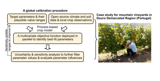
2. Materials and Methods

2.1. Observational Data

2.1.1. Field Measurements on Grapevine

The field data were collected in four experimental vineyard plots in the DDR by a viticulture observatory network, coordinated by the Association for the Development of Viticulture in the Douro Region (ADVID), Vila Real, Portugal. The geographical representation of these locations was already shown in Reis et al. [26]. In this study, there were 6-year consecutive measurements (2014–2019) available in each plot, relating to a particular combination of two local widespread used (autochthonous) varieties: Touriga Franca (TF) and Touriga Nacional (TN), arranged in two commonly applied training systems: single (unilateral) and double (bilateral) cordon, both with spurs pruned (Table 1). To account for the distinction between the training systems in the model, we have outlined several relevant model parameters (Table 1). Representative parameter values (mostly identical) were defined between single and double cordon according to a local expert’s technical knowledge (except planting density was via direct measurements). These values were also found to be consistent with the available published data (e.g., trunk height and inter-row distance) [23,27]. However, the initial plant growth status, in terms of carbon and nitrogen reserves, was estimated as a function of planting density and type of training system, according to the method developed by Bates et al. [28]. For the growth parameters (Table 1), the measurements were carried out over 20 randomly selected plants (replicates), for each plot and year (Table S1). Accordingly, the annual yield (kg/ha) at harvest was calculated as the median cluster number per vine × median cluster weight × planting density. Since the harvestable cluster number per vine happened to be a direct model input parameter (variety–training system specific), a locally representative value was defined by using additional plot measurements (Table S1). The representative value was fixed (median of all measurements) to describe the general characteristics for each variety–training system, e.g., the cluster number was generally lower in the single cordon than in the double cordon (Table S1). For the phenology data (Table 1), day of year (DOY) for flowering was recorded when 50% of the plant samples (5–10 vines) reached the flowering stage. A more detailed description of flowering data can be found in Reis et al. [26]. The harvest DOY was determined when most of the plants in the plots reached oenological maturations with the desired quality (balanced berry compounds). In particular, the berry sugar concentration was regularly measured between August and September to allow estimations of potential alcohol content (variability was discovered between years and sites), which shall not exceed 14° to ensure local vine characteristics. Other factors, such as pests and diseases, are regularly monitored. In case of occurrence, the necessary measures (e.g., fungicidal or insecticidal agents) were taken to minimize their influence.

2.1.2. Weather and Soil Inputs

The required weather and soil inputs for the vineyard sites were both extracted from gridded datasets, which were previously shown to be useful for reliable simulations of STICS at both the field and regional level [29,30,31,32]. Recent versions were used to reflect the data update and improvement. Specifically, the recent release of the E-OBS gridded dataset, v21.0 e [33], as well as the ERA5-Land hourly reanalysis dataset [34] were utilized to provide the required inputs of the meteorological variables at an enhanced spatial resolution (0.1° × 0.1°). The raw meteorological data were then processed into the model-required format following common agrometeorological approaches [35], which are described in detail in the Supplementary Material. The mean temperature and precipitation sum during the grapevine growing season (April–October) were plotted for the four sites for the period 2014–2019, showing a considerable inter-annual variability (including the anomaly warm and dry year 2017) (Figure S1). Therefore, the data were obtained under a broad range of weather conditions (very dry to wet). To account for complex local terrain conditions, a regional topography dataset at a resolution of ~25 m was introduced to supply site-specific information of the surface slope [36]. The use of gridded datasets for calibration, instead of in situ weather and soil measurements, was mainly due to the data scarcity. In particular, the employed E-OBS dataset represented a high-quality, openly accessible dataset, which was constructed using approximately 3700 and 9000 weather station data points for temperature and precipitation, respectively [33]. On the other hand, the advantage was to ensure consistency when the model was further implemented at a regional scale using gridded data inputs. For instance, the estimated parameters can be very different between a weather station and gridded weather data during calibration. However, using gridded datasets as inputs would implicitly assume an expectation of non-zero errors while trying to minimize the calibration errors. A multi-model study also applied gridded weather and soil datasets as inputs to optimize their calibration errors and obtained satisfactory results [37].

2.2. Brief Description of STICS Grapevine Modules

A brief description of the STICS (v9.1) modules concerning grapevine phenology and yield formation is presented here, whilst more comprehensive presentations of the model structure and formulations are available in Garcia de Cortazar Atauri [38] and Brisson et al. [16]. The phenology phase between dormancy and budburst was simulated using the BRIN model [39], whereas the subsequent stages, such as flowering, veraison and fruit maturity, were simulated using the classic growing degree day model with the base temperature of 10 °C [16]. Different temperature thresholds were also utilized for simulating frost damage and heat shocks in several critical stages (e.g., fruit setting) [16]. The harvest decision can be based on berry water content, which is mainly related to plant water status and the asynchronous nature of berry maturation, characterized by different berry phenology stages (fruit age classes) [40]. However, the simulation of berry water content can be influenced by potential berry shriveling with high-temperature episodes. The yield simulation also considered the asynchronous dynamic of fruit growth using a boxcar train technique, which was mainly temperature-driven and integrated the abiotic stress effects [16]. A more detailed description of the growth and yield formation modules is available in the Supplementary Material.

2.3. Calibration Setup

2.3.1. Identification of the Calibrated Parameters

The calibration was performed for the output variables of flowering, harvest dates and grapevine yield (kg/ha). We firstly specified a range for each parameter, according to expert experience and knowledge, which generally covered a wide range of local conditions, e.g., the potential dry berry weight parameter (Table 2). Secondly, the interval for each parameter range was specified, taking into account a trade-off between computation workloads and calibration demands. Here, we evenly sampled seven genotype-dependent and two plant-dependent parameters with 5 and 3 different values, respectively, with a total of 703,125 combinations tested for each site (Table 2). The selected genotype parameters already represent the large majority of available variety-specific parameters. The remaining ones (e.g., chilling requirement for dormancy break) were considered less relevant and fixed according to the previous analysis by Fraga et al. [21]. For generic parameters, fruit-age classes (nboite) ware chosen because it is closely related with parameters of fruit-setting duration (stdrpnou), fruit growth dynamics (dureefruit, pgrainmaxi) and fruit water dynamics (stdrpdes) [16], which are listed in Table 2. The threshold value of the source/sink ratio (spfrmin) (Table 2) represents the sensitivity (increased sensitivity with a higher value) of the fruit number formation to environmental stresses, indicating the limit below which the fruit-setting (sink growth) process was constrained, e.g., the source provision from photosynthesis assimilates did not satisfy the growth demand [16]. In the present study, harvest date was simulated assuming the berry water content reached 77%, which can be assimilated to a mean sugar concentration of ~21.0 °Brix (close to local wine characteristics) using equations established by García de Cortázar-Atauri et al. [40]. All parameters had either direct or indirect effects in simulating the yield and harvest date, whereas the flowering date was affected by only one parameter (stlevdrp) (Table 2).

2.3.2. Establishment of the Unit of Simulation (USM) and Objective Function

The USM notion in STICS represented the basic simulation unit, where one USM simulated a single crop growth cycle under a given soil, climate and management (i.e., single site–season–treatment combination) [6,16]. Altogether, we had 4 sites × 6 seasonal measurement combinations (24 USM), which was comparable to 27 combinations in a calibration study for rice [10].
The prediction uncertainty was generally defined as the distribution of prediction error around the observed value [11]. A convenient summary of the error distribution can be based on common statistical metrics, such as MSE. In this study, we adopted one of the frequentist methods, described in detail by Buis et al. [41] and Wallach et al. [25], with user-specified weights to combine the different response variables with a non-zero error expectation. However, modifications were made to the initial objective function by replacing the MSE component with nRMSE (%), which was written in Equation (1) as
θ ^ = argmin θ j ω j i , k [ Y i j k f j k ( X i ; θ ) ] 2 n i j × 100 Y j m e a n
where Y i j k is the observed value for a specific output variable j at the k-th measurement date for the i-th USM (herein only one measurement per season for each variable); f j k ( X i ; θ ) is the STICS model prediction, based on a given parameter vector θ out of the pre-defined 703,125 vectors; X i represents all the input variables for the i-th USM;
i , k [ Y i j k f j k ( X i ; θ ) ] 2 n i j × 100 Y j m e a n (nRMSE) summarizes the inter-annual variations in errors for a single response variable j; nij is the number of USM where the response variable j was measured (i.e., an equally 6-year measurement for both phenology and yield at each plot); Y j m e a n is the mean observation for the response variable j; and ω j is the user-defined weight for each response variable. The weight given to each variable determines the priority given to the prediction accuracy of that response variable, i.e., a higher weight for a higher priority [25]. We followed here an equal-weight approach ( ω j = 1), thus giving equal importance to phenology and yield.
As aforementioned, this was a multivariate objective function, enabling to combine prediction uncertainties on phenology and yield in the same dimension expressed as percentage errors (%) (lower value indicated less residue variance). The aim is to look for the parameter vector (among tested vectors) that minimized the sum of nRMSEflower + nRMSEharvest + nRMSEyield for each studied variety–training system. The normalization by the mean observation, rather than the range, is widely used in crop modelling communities [6,29,42], thus facilitating comparisons between studies. Furthermore, in standard regression analysis, the MSE of the prediction already integrated the effects of parameter uncertainties and variance in model error [10]. In this study, the total prediction variability was caused by parameter variability, where the total variability included a fixed contribution of the model error term. For a given subject (i.e., variety–training system), the fixed model error term (for every calculated nRMSE) included the uncertainties from the model structure (e.g., equations not exhaustively included all explanatory variables), input variables (limited accuracy in gridded datasets), and the measurement errors.

2.3.3. Assumption of Error Distributions

The defined objective function was analogous to the single-stage OLS parameter estimation [43]. The theory behind OLS is that all the model errors are independent with equal variance [43]. However, we assumed that the errors between the different response variables, measured at the same site in different years, could be correlated [10], along with unequal variance, as the inter-annual variability likely differed between phenology and yield. Yet the assumptions were unlikely constant, which can vary with the tested parameter vectors (see results). A data transformation might be required before summing nRMSE over different variables, e.g., by decomposition of the variance–covariance matrix of model errors to transform both the observed and simulated values [10]. To avoid such complexity and possibly high computation workloads, we also searched for parameters that separately minimized the nRMSE of each response variable, i.e., a univariate function. The purpose is to compare if the parameter vector that minimized the sum of the nRMSE can also minimize the nRMSE of each variable. In case not, it is of interest to see if they can produce a trade-off to achieve a prediction accuracy close to the best possible fit of each response variable.

2.3.4. Parameter Uncertainty and Sensitivity Analysis

For calibration, we have selected the most relevant parameters with pre-defined value ranges, and then searched for the best-fitted parameter vector with the defined objective function. This approach is generally consistent with the existing framework of model calibration [7]. Additionally, a simple and straightforward analysis was carried out to evaluate how individual parameter values can determine the total prediction variabilities. This was achieved by simply fixing a given parameter value and plotting the distribution of the nRMSE over the remaining parameter combinations (Figures S2–S5). From this distribution, the lowest possible nRMSE, achieved within values of a given parameter, as well as the corresponding nRMSE ranges (spread) can be assessed (Figures S2–S5). Subsequently, we investigated for each parameter if a particular value that resulted in the lowest nRMSE could simultaneously lead to the smallest uncertainty range (denoted as stable calibration), or lowest nRMSE but with the largest uncertainty range (denoted as unstable calibration). This approach provided information on the overall performance of a parameter value given the model, rather than only focusing on if it could minimize the errors. However, we still stick to the parameter values that can minimize the sum of the nRMSE, since we intended to minimize the prediction uncertainties for a specific situation (i.e., variety–training system). The unstable calibration (or stable calibration) just provided extra information on whether (or not) a calibrated parameter, obtained by minimizing the sum of nRMSE, was meanwhile susceptible to the influence from other parameters. This would be useful when there were multiple best-fit parameter values, where the stable calibrated values shall be preferentially selected.
A global sensitivity analysis was performed to evaluate the relative importance of each parameter in terms of its effect on the total variance of prediction uncertainty [44]. For each variety–training system, a variance-based sensitivity index was calculated based on the distribution of the nRMSE (among all tested parameter vectors), rather than the distribution of the direct simulation output. Thus, it reflected the parameter sensitivity to both environmental conditions and observational data. The index was calculated as the ratio of the variance in the expected nRMSE of a given parameter (i.e., the variance across the different mean nRMSE values obtained by a range of values within a given parameter) to total variance of the nRMSE due to variations in all parameters. The index corresponded to the main effect index of each parameter, as indicated by Sexton et al. [44], representing the expected reduction in total variance if a given parameter was known beforehand.

2.4. Evaluations of Calibrated Parameters

2.4.1. Goodness-Of-Fit of the Estimated Parameters

Since no single measure could comprehensively assess the model performance alone, it was essential to use additional statistic metrics, on top of the nRMSE, to better examine how well the calibrated model (with the best-selected parameters) can reproduce the observations [10]. The simulations were generally considered excellent, with an nRMSE below 10%; good when the nRMSE was between 10% and 20%; fair between 20% and 30%; and poor if it was greater than 30% [42]. However, these criteria can be applied for yield simulations but not for phenology. For instance, a 13% nRMSE in flowering date could correspond to a mean prediction bias of −18 days (see results), which indeed was a poor performance. Thus, three complementary statistical metrics were proposed: Mean Biased Errors (MBE), Mean Absolute Errors (MAE) and Ratio of Standard Deviations (Rsd). MBE measured the average bias (under- or overestimation) of the model, while MAE indicated the average magnitude of the absolute errors [15]; the Rsd (ratio of simulated to observed SD) allowed to estimate the model capacity to reproduce the observed data variability [6].

2.4.2. Evaluations Using Additional Published Data

Independent evaluations of the calibrated model were carried out using additional published data (both phenology and yield), which were assessed using the same goodness-of-fit metrics. The data was obtained from a vineyard plot within the DDR (different from the calibration sites), but comprising only the double-cordon training system between the two varieties and over a 2- or 3-year period [21]. Additionally, since these data were previously used for calibration of the same model but with a trial-and-error approach [21], it offered an opportunity to compare if the parameters resulting from a systematic calibration approach can lead to a better prediction performance or not. Therefore, the calibration procedures illustrated in Section 2.3 were repeated for the evaluation data to allow comparison with those from Fraga et al. [21].

2.5. Data Process and Software Environment

Both observed and simulated data were processed and analyzed in the Python (v3.8) environment, mainly based on the Numpy (v1.18.5) and Panda (v1.0.5) libraries. The boxplots for the distribution of the nRMSE and related bar plots, as well as the parallel coordinate plots were all produced using Matplotlib (v3.2.2). The iterations across all of the tested parameter vectors were developed and configured to run in parallel with multiple processors, according to the Message Passing Interface (MPI, v3.0.3) for the Python package. An individual iteration was made possible thanks to the convenient JavaStics (v1.4.1) command-line tool that enabled running a different USM per parameter vector. The parallel implementation was accomplished at the High-Performance Cluster at PIK (HPC@PIK) in a Linux environment.

3. Results and Discussion

3.1. General Assessment of Testing Parameters

3.1.1. Total Spread of Prediction Uncertainties

There is considerable spread of the nRMSE (21–315%) for the yield simulations among the tested parameter vectors (684,375) for different variety–training systems, whereas the spread for the phenology variables (1% to ~20%) is relatively small (Figure 1a). As a result, the variable combining phenology and yield (i.e., objective function) tends to have a large spread, mostly due to the yield variability (Figure 1a). However, the smaller spread for phenology can be mostly attributed to the inherently lower sensitivity of the nRMSE to phenology variations expressed in DOY (the denominator is a much larger value than the numerator). For phenology predictions, all the parameters result in an nRMSE below 20%, with median values varying from 4% to 8% (Figure 1b). In contrast, the median nRMSE for yield ranges from 51% to 106% (Figure 1a). Nonetheless, considering an nRMSE below 30%, not rated as a poor performance for yield simulations [42], there is still a reasonable amount of parameter vectors (330 to 5442) available for each variety–training system (Figure 1b). In this case, the median and min nRMSE is 28–29% and 21–25%, respectively, along with a smaller spread across the variety–training system (Figure 1b). Overall, these findings suggest the model can adapt to distinctive terroir characteristics in the DDR to simulate grapevine phenology and yield, despite most of the parameter combinations not having a good predictive skill for yield. Indeed, for process-based models such as STICS, one of the inherent limitations of yield simulation is the difficulty to adequately take into account the in-field variability [45]. Considerable spatial (in-plot) variability is observed for the measured cluster number/vine at harvest (Table S1), where we prescribe the model with a fixed representative value per variety–training system. As such, the discrepancy between the observed and simulated yield can be mostly explained by the fact that the former is based on the actual measured cluster number/vine (varied yearly). Nevertheless, this is essential for practical applications in future studies given the difficulty to measure this parameter, as the cluster number/vine not only depends on the variety–training system but is also affected by viticulture practices (e.g., pruning and cluster removal) and latent bud fertility [38]. The large in-field variability is associated with complex topography conditions in the DDR, where the steep vineyard slope can result in heterogeneous crop water availability [20,21]. Hence, to reduce model structure uncertainties, further improvements, e.g., via introducing an additional runoff process [46], may be needed to account for more detailed characteristics of the mountainous viticulture in the DDR.

3.1.2. Error Dependence and Homoscedasticity Test

There is generally a large variability in the error correlation (no to significant) between the variables among all the parameter vectors, while the error variance between flowering and harvest DOY also vary with the parameters (but an unequal variance is constantly found between phenology and yield) (Figure S6 with detailed descriptions). This suggests that a constant assumption of model errors, without considering possible parameter-induced variations, can be incorrect. Moreover, a common method to correct error correlation and heteroscedasticity is to do OLS only after a transformation to independent errors with homoscedasticity, which essentially corresponds to the generalized least squares (GLS) method [10]. However, Wallach et al. [10] also demonstrated the GLS method can result in larger parameter uncertainties than the OLS method. Liu et al. [14] simply use a one-stage OLS method to achieve a satisfactory parameter estimation despite having error dependence between sites.

3.2. Calibration Results

3.2.1. Calibrated Parameters and Associated Uncertainties

Based on the distribution of the nRMSE under each parameter value (Figures S2–S5), we presented its minimum (Figure 2) and range values (Figure 3) based on the objective function. Parameters minimizing the sum of the nRMSE show a slightly better performance for TN (31.0% and 29.5%) than for TF (33.9% and 38.2%) between the single- and double-cordon systems (Figure 2). These minimum values are identical throughout the parameters, serving as the criteria to choose the parameter values with the best possible fit. For instance, FF1500 is preferably chosen rather than FF900 for TN with the double-cordon system (Figure 2b). On the other hand, the overall prediction variability can be reduced if certain parameter values are used; e.g., FN0.5 rather than FN2.5 can reduce the spread of the nRMSE from 240% to 92% (Figure 3a). Comparatively, the total variability is smaller for TF with the single-cordon system (Figure 3c), also reflected in Figure 1a, which may be due to its relatively small variation in yield data (Table 1). The parameters can thus be selected to potentially have less dispersion (“noise”) in the predictions. However, in most cases, the parameter values that minimize the spread do not simultaneously minimize the nRMSE (Figure 2 and Figure 3).
A list of calibrated parameters for each variety–training system, along with the denoted stable or unstable calibration (Section 2.3.4), is presented in Table 3. Note that when a given parameter is neither stable nor unstable according to the proposed definitions, its uncertainty information can be directly referred to in Figure 3. A fairly common situation in crop model calibration is the difficulty to choose the optimal parameter combination when there are several choices with equally good performance [8]. Our study herein presents a new method to characterize the parameter uncertainty, e.g., different from the methods to quantify the uncertainties with standard deviation [10,14]. This approach can allow one to choose the best-fitted parameters when multiple choices with equal performance occur. For instance, all SS values simulate equally for TN with a single-cordon system, but SS0.75 (stable calibration) is preferably chosen for its role in reducing the spread of nRMSE caused by uncertainties in the other parameters (Table 3 and Figure 3a). The same applies to WD, where unstable calibrated values can be excluded (Table 3 and Figure 3b,c). Admittedly, this approach relies on the prior information of the parameters and sometimes it can be very vague [14]. We combined the expert knowledge of the model with information from local viticulturists to pre-define the parameter value range. Sexton et al. [44] defines the prior range of values for 10 parameters using the APSIM-Sugar model for a global sensitivity analysis. A more sophisticated method, such as the phenotyping of genotype-dependent parameter ranges, might be necessary to better represent the genotypic variability [47].

3.2.2. Sensitivity Analysis and Interpretation of Calibrated Parameters

Flowering date simulation, as explained before, is only determined by one testing parameter (RG) (Figure 4a), which is involved in the GDD model [16]. For harvest date, BN, FS, FF, RG and WD are generally the most sensitive parameters, despite different sensitive magnitudes between plots (Figure 4b). This is as expected, since BN defines the berry growth stages and WD initializes the fruit water dynamic, while the other three parameters directly relate to the thermal requirements from budburst to maturity (Table 2) [16]. For yield simulations, FS is generally the most sensitive parameter, followed by FN, FW or RG, respectively (Figure 4c). These parameters were known to play important roles in yield simulations, in which FS, identified as the most influential parameter, acted synchronously with FN, BN and the cluster number to determine total fruit number [16]. It hints toward the model tending to put more emphasis on fruit number rather than fruit weight (mostly controlled by FW) as the yield determinant in the DDR. For the combined variable, the relatively sensitive parameters are the same as those for yield (Figure 4d), since the sum of the nRMSE mostly come from yield simulations. Note that a very low sensitivity index (close to zero for VG and SS) does not indicate no effects for the parameter (Figure 4b,c), but rather a relatively low sensitivity [44]. For instance, harvest DOY and yield simulations are different between values of VG and SS (Figures S7–S10). VG mainly defines the length of the LAI growth period (stops after veraison). Under a similar Mediterranean environment, it was found that an inaccurate estimation of LAI before veraison in STICS might not significantly affect the final yield estimations [48]. The limited influence of SS is probably because the fruit-setting phase generally takes place in a less warm and dry period (middle-May to middle-June). Increased SS sensitivity is possible if higher RG values beyond the current range are tested, i.e., shift the fruit-setting stage into an unfavorable period. Sensitive parameters for phenology and yield can also be reflected from the calculated spread of the nRMSE for each variable (Figures S7–S10). Less sensitive parameters seem to have more uncertainties in estimating the best-fit values, as different values are prone to having the same results, e.g., VG, WD and SS in Table 3.
Calibration, found by simply fitting the model to field data, though adapting the model to a specific target population, can lead to estimated parameters that lack physiological meaning [47]. The fixed harvestable cluster number/vine with a representative value (Table S1), to some extent, is at the expense of meaningful values for other parameters in order to improve the model fit to the observed data. This can essentially explain the absence of a difference in the potential dry berry weight (0.5 g) between the two varieties. However, it is also possible, as the difference was only observed for fresh berry weight (dominated by water content) [49]. Besides, this parameter was previously set to 0.66 g for the Cabernet Sauvignon variety (higher productivity than current varieties) in a dry Mediterranean environment [48]. Yet, reasonable parameter values are still found for FN (Table 3), where it is recognized that variety TF displays a higher fruit growth potential than TN [21,49].
RG is calibrated to nearly the same values as those by Fraga et al. [21] in the DDR, and slightly lower values are obtained for VG. However, FS and FF are defined with higher values than the previous case [21], perhaps to compensate for the low FW values. The remaining parameters are mostly difficult to link to the observed data (WD, BN and SS), as is common for crop models [8]. Furthermore, there is a need to have more detailed seasonal measurements for other growth variables, e.g., LAI, aerial biomass and yield components, to enable studying the model processes individually where each process is associated with only a few participatory parameters to calibrate.

3.2.3. Comparison between Multivariate and Univariate Function

Once the parameters have been estimated, it is essential to evaluate the calibrated model performance using various goodness-of-fit measures. Firstly, the results consistently indicate that the parameters minimizing the nRMSE for phenology and yield are different (more details are available in Figures S7–S10). Thus, different parameters are identified between the multivariate and univariate function for all variety–training systems (Table 3). It is simply because there is no such a parameter vector θ that achieves the minimum prediction errors for phenology and yield simultaneously. This is indeed a common situation for a complex model such as STICS when the model does not fully describe the dependence on the explanatory variable and has a non-zero expectation of errors [25,41]. The evaluation results further indicate that the estimated parameters from the multivariate objective function generally perform much better than those from the univariate function (Table 4). The former results in a negligible MBE and good results for the MAE: the MBE is −2 to 4 days for phenology and −232 to 159 kg/ha for yield, while the MAE is 3 to 6 days (except 10, 12 days for harvest DOY under TF) and 1168 to 1417 kg/ha (Table 4). The variance in the observed data is generally well reproduced: the average Rsd is 0.99, varying from 0.6 to 1.5, except for TF with a single cordon (overestimate the inter-annual variability for flowering DOY and yield) (Table 4). Overall, the calibrated model achieves a satisfactory performance, while the performance is better for TN than for TF for the two training systems. The results are comparable to a STICS evaluation study (adapted for Cabernet Sauvignon and Aranel) carried out in similar Mediterranean climates (e.g., seasonal rainfall <350 mm): the bias for phenology is no more than 6 days and 500–2600 kg/ha for yield [48]. However, the difference is that the grapevine yield of the DDR is much lower (4–9 t/ha) than that of the study (10–17 t/ha) [48]. Therefore, our study contributes to demonstrate the model’s usefulness for simulating grapevine phenology and yield under a low production environment.
In contrast, parameters minimizing the prediction errors for yield have a significant bias for phenology (e.g., MBE for flowering DOY varies from −16 to −22), and vice versa (nRMSE for yield varies from 56% to 198%) (Table 4). Thus, we should not rely on the parameters identified from the univariate function unless the model is exclusively used for simulating a single response variable. On the other hand, the estimated parameters from the objective function achieve results close to the best possible fit of each response variable: near-minimum errors for harvest DOY and yield but with minimized errors for flowering DOY (Table 4). The difference from the obtained minimum nRMSE is 0–4% for harvest DOY and 3–6% for yield, while such a difference for MAE is 0–9 days and 122–188 kg/ha, respectively (Table 4). The difference from the best obtained Rsd is 0.1–0.5 for harvest DOY and 0–0.4 for yield (Table 4). These results are in line with Wallach et al. [25], which suggest that the best fit to one response variable can lead to a poor fit to the other variables, while a good compromise is to have the parameter-fitting simulations close to the optimum of each variable. Compared to previous studies, we have adopted a similar statistical model of errors, but a very different numeric method to implement [14,25,41]. For example, Liu et al. [14] apply the Gauss–Newton algorithm in a frequentist approach to search for the parameters that minimize the SSE over two phenology phases. Such a gradient-based minimization method, though with a stringent convergence test, requires the simulated values to be a continuous function of the estimated parameters, which is very difficult to apply to crop models with multiple discontinuities and non-linearities [8,25].
Overall, our method is relatively simple and straightforward without specific requirements (e.g., model continuity or multiple starting points for parameter estimations), which allow rapidly testing a large number of parameter combinations for different response variables (<24 h for 684,375 combinations), thanks to the parallel feature of the algorithm. However, it is important to highlight that the estimated parameter vector might not be the optimal choice given the data, but rather the best-fitted one from the pre-defined parameter value range (assumed to be a large parameter sample drawn from its population). A possible remedy is to repeat the same objective function with an updated range of parameter values with a smaller interval around the estimated values. This can be repeated several times to continuously reduce the errors until no improvements are observed. However, this should be done only if the goodness-of-fit results are not satisfactory. Herein, we only had one repeat for TF with the single-cordon system, which reduced the minimum sum of the nRSME from 34% to 30% (not shown).

3.3. Variations in the Best-Performing Parameters among Variety–Training Systems

It is crucial to check whether the model adapts substantially different from one variety–training system to another (e.g., the best-predicted parameters for one system show poor performance for others), as the identified parameters can simply be the result of a random choice. The analysis reveals that these best-fit parameter vectors (except for TF with the single-cordon system) (Table 3) tend to converge for the other variety–training systems, i.e., the prediction performance (nRMSE) generally falls within a common narrow range (Figure 5a). This can also be seen for predictions on flowering DOY, where the calibrated RG values are almost identical (either 300 or 250) across the variety–training system (Table 3). Moreover, apart from TF with a single cordon, the 5% best-performing parameter vectors (in terms of nRMSE) for one variety–training system are generally within the 15% best-performing vectors for another one (Figure 5b). This illustrates that the model’s potential adaptation skill is similar across variety–training systems, by which only a certain fraction of the parameter combinations is relevant for local phenology and yield simulations (from which the best-fit values are estimated). Regarding the exception of TF with a single-cordon system, we speculate it might be associated with the very different inter-annual variability in the observed yield (Table 1). This can be due to data measuring problems or special practices applied (e.g., supplemental irrigation in dry years), but without detailed records.

3.4. Evaluations Using Additional Data

The calibrated model shows particularly satisfactory performance for yield predictions using additional evaluation datasets (Table 5). The performance is better than that in the calibration datasets (but probably not comparable given different sample sizes) (Table 4 and Table 5), which is slightly better than in a previous study where STICS is differently calibrated [21]. This reveals the importance of establishing a searching algorithm that approximates the best-fit parameter values, particularly in situations where the majority of the parameter combinations do not predict well (Figure 1a). The adequate yield-predictive skills in the DDR can be explained by appropriate simulations of plant water-stress conditions during the warm and dry season [21]. STICS is especially good at simulating total soil water content with an nRMSE of 10% over a wide range of agro-environmental conditions [6]. However, the calibrated parameters do not simultaneously provide good simulations on phenology, particularly for harvest DOY (Table 5). A fixed harvest criterion of expected alcohol content at 12.5° (converted from Brix value) was used to model its actual variability (10–14°) in observations during calibration. It is advantageous to demonstrate its representativeness and avoid specific inputs each time. The simulation is overall fair for the calibration data (though modest errors for TF) (Table 4), whereas poor predictions for the evaluation data can be possibly explained by limitations in simulating the measured berry alcohol content [21]. Indeed, using one specific criterion to model the harvest date is insufficient as it is determined by many quality parameters (e.g., sugar, acid, phenolic and aromatic compounds) in accordance with the expected wine style. Besides, external factors, such as logistic issue and workforce availability, can also affect the results. On the other hand, it is known that a better fit to the calibration data does not necessarily indicate better predictions for new situations [10,41]. Nevertheless, further model improvement should consider the various criteria of harvest decision-making for winegrowers (e.g., using a sugar/acid ratio).
Lastly, when the same calibration procedure is applied to the evaluation data, it is again demonstrated that for even a smaller size data sample, there is no parameter vector (θ) that can simultaneously minimize the prediction errors for phenology and yield (Table S2). The estimated parameters from the objective function can minimize the nRMSE for flowering DOY and yield (only TN), but not for harvest DOY (Table S2). Similar to the calibration data, the parameters with a minimum nRMSE for harvest DOY and yield are quite different for the evaluation data (Table S2). Indeed, harvest timings are more dependent on the desired grape quality rather than yield, for which the fruit water dynamic was independent of fruit dry mass simulations in STICS [16]. Nevertheless, the calibrated parameters show a considerable improvement in prediction accuracy (particularly for yield) compared to those previously estimated by the trial-and-error approach (Table S3).

4. Conclusions

Parameter estimations and their associated uncertainties are important for crop model applications in various fields, e.g., climate impact assessment. The employed calibration approach defines an objective function with a statistical model of errors to look for the best-fit parameter values from pre-defined ranges, which achieve the minimum values of the unweighted sum of the nRMSE across the phenology variables (flowering and harvest DOY) and grape yield at four vineyards in the DDR from 2014 to 2019. It is consistently found that there is no parameter vector that can simultaneously achieve the minimum prediction errors for phenology and yield across the different variety–training systems. However, the identified parameters can achieve results close to the best-possible fit of each variable with an overall satisfactory performance, where the MBE is negligible with −2 to 4 days for phenology and −232 to 159 kg/ha for yield. However, the variance in the observed data is not well reproduced for TF with a single cordon, suggesting the need for further improvements. The calibrated model is satisfactorily evaluated for yield simulations using additional data, but not for harvest date, highlighting the need for the model to have various harvest-criteria simulations.
The parameter uncertainties are characterized as to how a given parameter value can determine the total prediction variability caused by the uncertainties of other parameter combinations. Accordingly, unstable or stable calibrations are proposed, depending on if an estimated parameter value is susceptible to the influence of other parameters. This is particularly useful for selecting the best-fit parameter values when there are several choices with equally good performance. A global sensitivity analysis is applied to evaluate the relative importance of each parameter, which highlights the important role of the fruit-setting parameters as key determinants for yield simulations. These parameters are of particular interests to explore the response of specific plant traits (setting fruits) under climate change scenarios. Parameter sensitivity can also be obtained from a parameter uncertainty analysis, where the less-sensitive parameters tend to have more uncertainties in estimating the best-fit values. Overall, the approach is straightforward with a simple algorithm to implement, which is primarily based on testing a large number of parameter combinations. It is generally consistent with the existing framework for crop model calibration, which can be easily adapted for other models and crops. However, the major challenge to fit simulations using different types of response variables lies in the difficulty to have an appropriate assumption of the model errors. We demonstrate its complexity, since the assumption is also dependent on the testing parameters beyond if the measurements were made in the same plot. The present method might be combined with other approaches (e.g., Bayesian) and with more detailed seasonal measurements, to enable more comprehensive evaluations of the estimated parameters, thus contributing to a better understanding of the modelling system.

Supplementary Materials

The following are available online at https://www.mdpi.com/article/10.3390/agronomy11081659/s1. Table S1: Summary of the yearly measured cluster number per vine and individual cluster weight at harvest in four experimental vineyard plots from 2014 to 2019. Table S2: List of parameters that respectively minimize the sum of the nRMSE (%) based on the multivariate objective function and minimize the nRMSE for flowering and harvest date and yield separately (univariate function). Table S3: Goodness-of-fit comparison of the selected parameter vectors that minimize the sum of nRMSE (%) based on the objective function with parameter vectors previously selected with a trial-and-error approach. Figure S1: Mean temperature (°C) and precipitation sum (mm) during the growing season (between April and October) between 2013 and 2019 in the studied experimental vineyard plots. Figures S2–S5: Spread of prediction uncertainties (nRMSE, %) on phenology, yield and the combined variable (i.e., objective function) under individual parameter values for the four variety–training systems. Figure S6: Boxplots of error (observation-simulation) correlations between the studied variables and the Levene’s test on homoscedasticity. Figures S7–S10: Minimum and range values (spread) of the STICS model prediction uncertainties (nRMSE, %) under individual parameter values for phenology and yield separately over the four variety–training systems.

Author Contributions

Conceptualization and methodology, C.Y., C.M. and J.A.S.; software, C.Y. and C.M.; validation, all authors; formal analysis, all authors; investigation, all authors; resources, all authors; data curation, all authors; writing—original draft preparation, C.Y.; writing—review and editing, all authors; visualization, C.Y. and C.M.; supervision, C.M. and J.A.S.; project administration, J.A.S.; funding acquisition, J.A.S. All authors have read and agreed to the published version of the manuscript.

Funding

This study was funded through the Clim4Vitis project—“Climate change impact mitigation for European viticulture: knowledge transfer for an integrated approach”, funded by the European Union’s Horizon 2020 Research and Innovation Programme, under grant agreement no. 810176; It was also supported by FCT—Portuguese Foundation for Science and Technology, under the project UIDB/04033/2020. Nelson Machado and Samuel Reis kindly acknowledge funding by operation nº NORTE-06-3559-FSE-000067.

Institutional Review Board Statement

Not applicable.

Informed Consent Statement

Not applicable.

Data Availability Statement

Data is contained within the article or supplementary material. Specifically, the detailed yearly field measurements on several important grapevine parameters (e.g., cluster number and cluster weight) are presented in Table 1 and Table S1, respectively. Besides, the involved soil and climate datasets supplied as model inputs are from publicly available datasets (e.g., HWSD and E-OBS), where the data extraction and processing steps are described in detail in the Supplementary Material.

Acknowledgments

The authors acknowledge the kind help from Iñaki García de Cortázar-Atauri in diagnosing the model simulation problems. The authors also thank Cristina Carlos for availability during metadata queries. Finally, all authors are grateful for ADVID and their associates, for collaborations in data collections and provisions under the Viticulture Observatory of the DDR.

Conflicts of Interest

The authors declare no conflict of interest.

References

  1. Rötter, R.P.; Hoffmann, M.P.; Koch, M.; Müller, C. Progress in modelling agricultural impacts of and adaptations to climate change. Curr. Opin. Plant Biol. 2018, 45, 255–261. [Google Scholar] [CrossRef]
  2. Rosenzweig, C.; Jones, J.W.; Hatfield, J.L.; Ruane, A.C.; Boote, K.J.; Thorburn, P.; Antle, J.M.; Nelson, G.C.; Porter, C.; Janssen, S.; et al. The Agricultural Model Intercomparison and Improvement Project (AgMIP): Protocols and pilot studies. Agric. For. Meteorol. 2013, 170, 166–182. [Google Scholar] [CrossRef] [Green Version]
  3. Tao, F.; Palosuo, T.; Rötter, R.P.; Díaz-Ambrona, C.G.H.; Inés Mínguez, M.; Semenov, M.A.; Kersebaum, K.C.; Cammarano, D.; Specka, X.; Nendel, C.; et al. Why do crop models diverge substantially in climate impact projections? A comprehensive analysis based on eight barley crop models. Agric. For. Meteorol. 2020, 281, 107851. [Google Scholar] [CrossRef]
  4. Asseng, S.; Ewert, F.; Rosenzweig, C.; Jones, J.W.; Hatfield, J.L.; Ruane, A.C.; Boote, K.J.; Thorburn, P.J.; Rötter, R.P.; Cammarano, D.; et al. Uncertainty in simulating wheat yields under climate change. Nat. Clim. Chang. 2013, 3, 827–832. [Google Scholar] [CrossRef] [Green Version]
  5. Wallach, D.; Palosuo, T.; Thorburn, P.; Gourdain, E.; Asseng, S.; Basso, B.; Buis, S.; Crout, N.; Dibari, C.; Dumont, B.; et al. How well do crop modeling groups predict wheat phenology, given calibration data from the target population? Eur. J. Agron. 2021, 124, 126195. [Google Scholar] [CrossRef]
  6. Coucheney, E.; Buis, S.; Launay, M.; Constantin, J.; Mary, B.; García de Cortázar-Atauri, I.; Ripoche, D.; Beaudoin, N.; Ruget, F.; Andrianarisoa, K.S.; et al. Accuracy, robustness and behavior of the STICS soil–crop model for plant, water and nitrogen outputs: Evaluation over a wide range of agro-environmental conditions in France. Environ. Model. Softw. 2015, 64, 177–190. [Google Scholar] [CrossRef]
  7. Wallach, D.; Palosuo, T.; Thorburn, P.; Hochman, Z.; Gourdain, E.; Andrianasolo, F.; Asseng, S.; Basso, B.; Buis, S.; Crout, N.; et al. The chaos in calibrating crop models. bioRxiv 2020. [Google Scholar] [CrossRef]
  8. Seidel, S.J.; Palosuo, T.; Thorburn, P.; Wallach, D. Towards improved calibration of crop models—Where are we now and where should we go? Eur. J. Agron. 2018, 94, 25–35. [Google Scholar] [CrossRef]
  9. Wallach, D.; Thorburn, P.; Asseng, S.; Challinor, A.J.; Ewert, F.; Jones, J.W.; Rotter, R.; Ruane, A. Estimating model predic-tion error: Should you treat predictions as fixed or random? Environ. Model. Softw. 2016, 84, 529–539. [Google Scholar] [CrossRef]
  10. Wallach, D.; Nissanka, S.P.; Karunaratne, A.S.; Weerakoon, W.M.W.; Thorburn, P.J.; Boote, K.J.; Jones, J.W. Accounting for both parameter and model structure uncertainty in crop model predictions of phenology: A case study on rice. Eur. J. Agron. 2017, 88, 53–62. [Google Scholar] [CrossRef]
  11. Wallach, D.; Thorburn, P.J. Estimating uncertainty in crop model predictions: Current situation and future prospects. Eur. J. Agron. 2017, 88, A1–A7. [Google Scholar] [CrossRef]
  12. Bayarri, M.J.; Berger, J.O. The interplay of Bayesian and frequentist analysis. Stat. Sci. 2004, 19, 58–80. [Google Scholar] [CrossRef]
  13. Wallach, D.; Keussayan, N.; Brun, F.; Lacroix, B.; Bergez, J.-E. Assessing the Uncertainty when Using a Model to Compare Irrigation Strategies. Agron. J. 2012, 104, 1274–1283. [Google Scholar] [CrossRef]
  14. Liu, L.; Wallach, D.; Li, J.; Liu, B.; Zhang, L.; Tang, L.; Zhang, Y.; Qiu, X.; Cao, W.; Zhu, Y. Uncertainty in wheat phenology simulation induced by cultivar parameterization under climate warming. Eur. J. Agron. 2018, 94, 46–53. [Google Scholar] [CrossRef]
  15. Yang, J.M.; Yang, J.Y.; Liu, S.; Hoogenboom, G. An evaluation of the statistical methods for testing the performance of crop models with observed data. Agric. Syst. 2014, 127, 81–89. [Google Scholar] [CrossRef]
  16. Brisson, N.; Launay, M.; Mary, B.; Beaudoin, N. Conceptual Basis, Formalisations and Parameterization of the STICS Crop Model; Editions Quae: Versailles, France, 2009; ISBN 2759201694. [Google Scholar]
  17. Brisson, N.; Gary, C.; Justes, E.; Roche, R.; Mary, B.; Ripoche, D.; Zimmer, D.; Sierra, J.; Bertuzzi, P.; Burger, P.; et al. An overview of the crop model stics. Eur. J. Agron. 2003, 18, 309–332. [Google Scholar] [CrossRef]
  18. Fraga, H.; García de Cortázar Atauri, I.; Malheiro, A.C.; Santos, J.A. Modelling climate change impacts on viticultural yield, phenology and stress conditions in Europe. Glob. Chang. Biol. 2016, 22, 3774–3788. [Google Scholar] [CrossRef]
  19. Costa, R.; Fraga, H.; Fonseca, A.; De Cortázar-Atauri, I.G.; Val, M.C.; Carlos, C.; Reis, S.; Santos, J.A. Grapevine phenology of cv. Touriga Franca and Touriga Nacional in the Douro wine region: Modelling and climate change projections. Agronomy 2019, 9, 210. [Google Scholar] [CrossRef] [Green Version]
  20. Fraga, H.; Costa, R.; Santos, J.A. Multivariate clustering of viticultural terroirs in the Douro winemaking region. Cienc. Tec. Vitivinic. 2017, 32, 142–153. [Google Scholar] [CrossRef] [Green Version]
  21. Fraga, H.; Costa, R.; Moutinho-Pereira, J.; Correia, C.M.; Dinis, L.T.; Gonçalves, I.; Silvestre, J.; Eiras-Dias, J.; Malheiro, A.C.; Santos, J.A. Modeling phenology, water status, and yield components of three Portuguese grapevines using the STICS crop model. Am. J. Enol. Vitic. 2015, 66, 482–491. [Google Scholar] [CrossRef]
  22. Santos, J.A.; Ceglar, A.; Toreti, A.; Prodhomme, C. Performance of seasonal forecasts of Douro and Port wine production. Agric. For. Meteorol. 2020, 291, 108095. [Google Scholar] [CrossRef]
  23. Tosin, R.; Pôças, I.; Cunha, M. Spectral and thermal data as a proxy for leaf protective energy dissipation under kaolin application in grapevine cultivars. Open Agric. 2019, 4, 294–304. [Google Scholar] [CrossRef]
  24. Fraga, H.; Santos, J.A. Daily prediction of seasonal grapevine production in the Douro wine region based on favourable meteorological conditions. Aust. J. Grape Wine Res. 2017, 23, 296–304. [Google Scholar] [CrossRef]
  25. Wallach, D.; Buis, S.; Lecharpentier, P.; Bourges, J.; Clastre, P.; Launay, M.; Bergez, J.-E.; Guerif, M.; Soudais, J.; Justes, E. A package of parameter estimation methods and implementation for the STICS crop-soil model. Environ. Model. Softw. 2011, 26, 386–394. [Google Scholar] [CrossRef]
  26. Reis, S.; Fraga, H.; Carlos, C.; Silvestre, J.; Eiras-Dias, J.; Rodrigues, P.; Santos, J.A. Grapevine phenology in four portuguese wine regions: Modeling and predictions. Appl. Sci. 2020, 10, 3708. [Google Scholar] [CrossRef]
  27. Malheiro, A.C.; Pires, M.; Conceição, N.; Claro, A.M.; Dinis, L.T.; Moutinho-Pereira, J. Linking sap flow and trunk diameter measurements to assess water dynamics of touriga-nacional grapevines trained in cordon and guyot systems. Agriculture 2020, 10, 315. [Google Scholar] [CrossRef]
  28. Bates, T.R.; Dunst, R.M.; Joy, P. Seasonal dry matter, starch, and nutrient distribution in “Concord” grapevine roots. HortScience 2002, 37, 313–316. [Google Scholar] [CrossRef] [Green Version]
  29. Yang, C.; Fraga, H.; van Ieperen, W.; Santos, J.A. Assessing the impacts of recent-past climatic constraints on potential wheat yield and adaptation options under Mediterranean climate in southern Portugal. Agric. Syst. 2020, 182, 102844. [Google Scholar] [CrossRef]
  30. Yang, C.; Fraga, H.; van Ieperen, W.; Trindade, H.; Santos, J.A. Effects of climate change and adaptation options on winter wheat yield under rainfed Mediterranean conditions in southern Portugal. Clim. Chang. 2019, 154, 159–178. [Google Scholar] [CrossRef] [Green Version]
  31. Yang, C.; Fraga, H.; Ieperen, W.; Van Santos, J.A. Assessment of irrigated maize yield response to climate change scenarios in Portugal. Agric. Water Manag. 2017, 184, 178–190. [Google Scholar] [CrossRef]
  32. Yang, C.; Fraga, H.; Van Ieperen, W.; Santos, J.A. Modelling climate change impacts on early and late harvest grassland systems in Portugal. Crop. Pasture Sci. 2018, 69, 821–836. [Google Scholar] [CrossRef]
  33. Cornes, R.C.; van der Schrier, G.; van den Besselaar, E.J.M.; Jones, P.D. An Ensemble Version of the E-OBS Temperature and Precipitation Data Sets. J. Geophys. Res. Atmos. 2018, 123, 9391–9409. [Google Scholar] [CrossRef] [Green Version]
  34. Hersbach, H.; Bell, B.; Berrisford, P.; Hirahara, S.; Horányi, A.; Muñoz-Sabater, J.; Nicolas, J.; Peubey, C.; Radu, R.; Schepers, D.; et al. The ERA5 global reanalysis. Q. J. R. Meteorol. Soc. 2020, 146, 1999–2049. [Google Scholar] [CrossRef]
  35. Allen, R.G.; Pereira, L.S.; Raes, D.; Smith, M. Crop Evapotranspiration—Guidelines for Computing Crop Water Requirements—FAO Irrigation and Drainage Paper 56; FAO: Roma, Italy, 1998; ISBN 9251042195. [Google Scholar]
  36. LEAF (ex-CEAP). Declives de Portugal Continental. LEAF/ISA/ULisboa. Disponível. 2013. Available online: http://epic-webgis-portugal.isa.utl.pt/ (accessed on 30 June 2020).
  37. Liu, H.; Pequeno, D.N.L.; Hernández-Ochoa, I.M.; Krupnik, T.J.; Sonder, K.; Xiong, W.; Xu, Y. A consistent calibration across three wheat models to simulate wheat yield and phenology in China. Ecol. Modell. 2020, 430, 109132. [Google Scholar] [CrossRef]
  38. Garcia de Cortazar Atauri, I. Adaptation du Modèle STICS à la Vigne (Vitis vinifera L.): Utilisation dans le Cadre D’une Étude D’impact du Changement Climatique à L’échelle de la France. Ph.D. Thesis, Montpellier SupAgro, Montpellier, France, 2006. (In French). [Google Scholar]
  39. García de Cortázar-Atauri, I.; Brisson, N.; Gaudillere, J.P. Performance of several models for predicting budburst date of grapevine (Vitis vinifera L.). Int. J. Biometeorol. 2009, 53, 317–326. [Google Scholar] [CrossRef]
  40. García de Cortázar-Atauri, I.; Brisson, N.; Ollat, N.; Jacquet, O.; Payan, J.-C. Asynchronous dynamics of grapevine (“Vitis vinifera”) maturation: Experimental study for a modelling approach. OENO One 2009, 43, 83–97. [Google Scholar] [CrossRef]
  41. Buis, S.; Wallach, D.; Guillaume, S.; Varella, H.; Lecharpentier, P.; Launay, M.; Guérif, M.; Bergez, J.-E.; Justes, E. The STICS Crop Model and Associated Software for Analysis, Parameterization, and Evaluation. Methods Introd. Syst. Model. Agric. Res. 2011, 2, 395–426. [Google Scholar]
  42. Jamieson, P.D.; Porter, J.R.; Wilson, D.R. A test of the computer simulation model ARCWHEAT1 on wheat crops grown in New Zealand. F. Crop. Res. 1991, 27, 337–350. [Google Scholar] [CrossRef]
  43. Seber, G.A.F. Nonlinear Regression Models. In The Linear Model and Hypothesis: A General Unifying Theory; Springer International Publishing: Cham, Switzerland, 2015; pp. 117–128. ISBN 978-3-319-21930-1. [Google Scholar]
  44. Sexton, J.; Everingham, Y.L.; Inman-Bamber, G. A global sensitivity analysis of cultivar trait parameters in a sugarcane growth model for contrasting production environments in Queensland, Australia. Eur. J. Agron. 2017, 88, 96–105. [Google Scholar] [CrossRef]
  45. Kersebaum, K.C.; Boote, K.J.; Jorgenson, J.S.; Nendel, C.; Bindi, M.; Frühauf, C.; Gaiser, T.; Hoogenboom, G.; Kollas, C.; Olesen, J.E.; et al. Analysis and classification of data sets for calibration and validation of agro-ecosystem models. Environ. Model. Softw. 2015, 72, 402–417. [Google Scholar] [CrossRef]
  46. Roux, S. How sensitive is a vineyard crop model to the uncertainty of its runoff module? Environ. Model. Softw. 2017, 97, 86–92. [Google Scholar] [CrossRef]
  47. Casadebaig, P.; Debaeke, P.; Wallach, D. A new approach to crop model calibration: Phenotyping plus post-processing. Crop. Sci. 2020, 60, 709–720. [Google Scholar] [CrossRef]
  48. Valdés-Gómez, H.; Celette, F.; García de Cortázar-Atauri, I.; Jara-Rojas, F.; Ortega-Farías, S.; Gary, C. Modelling soil water content and grapevine growth and development with the stics crop-soil model under two different water management strategies. OENO One 2009, 43, 13–28. [Google Scholar] [CrossRef] [Green Version]
  49. Singh, R.K.; Afonso, J.; Nogueira, M.; Oliveira, A.A.; Cosme, F.; Falco, V. Silicates of Potassium and Aluminium (Kaolin); Comparative Foliar Mitigation Treatments and Biochemical Insight on Grape Berry Quality in Vitis vinifera L. (cv. Touriga National and Touriga Franca). Biology 2020, 9, 58. [Google Scholar] [CrossRef] [PubMed] [Green Version]
Figure 1. Spread of the STICS model prediction uncertainties (nRMSE, %) for each variety–training system on flower and harvest DOY, yield (kg/ha) and the objective function (combined phenology and yield), respectively. Spread over (a) all the tested parameter vectors (684,375 effective combinations); and (b) selected parameter vectors resulting in an nRMSE (%) below 30% (dash line), where the figures in the brackets indicate the corresponding number of available vectors. Refer to Figure S2 for the boxplot definition. TN: Touriga Nacional; TF: Touriga Franca (TF).
Agronomy 11 01659 g001
Figure 2. Minimum value of the STICS model prediction uncertainties (nRMSE, %) based on the combined variable (i.e., objective function) under each parameter value (fix a given parameter value and test the remaining combinations). (a) Touriga Nacional (TN) with the single-cordon training system; (b) Touriga Nacional (TN) with the double-cordon training system; (c) Touriga Franca (TF) with the single-cordon training system; (d) Touriga Franca (TF) with the double-cordon training system. The parameter abbreviations are denoted for each subplot (see Table 2 for detailed parameter descriptions). The associated boxplots are shown in Figures S2–S5. The calibrated parameters are BN: Box number; FF: Fruit filling thermal requirement; FS: Fruit setting thermal requirement; FN: Fruit number formation potential per degree day−1 per cluster; FW: Fruit (berry) weight potential; RG: Thermal requirement between budbreak and reproductive onset; SS: Source sink ratio threshold; VG: Thermal requirement between juvenile onset and veraison onset; WD: Thermal requirement between reproductive onset and fruit water dynamic onset.
Agronomy 11 01659 g002
Figure 3. Range of STICS model prediction uncertainties (nRMSE, %) based on the combined variable (i.e., objective function) under each parameter value (fix a given parameter value and test the remaining combinations). (a) Touriga Nacional (TN) with the single-cordon training system; (b) Touriga Nacional (TN) with the double-cordon training system; (c) Touriga Franca (TF) with the single-cordon training system; (d) Touriga Franca (TF) with the double-cordon training system. The range (spread) is calculated as four times the inter-quartile range (the associated boxplots are shown in Figures S2–S5).
Agronomy 11 01659 g003
Figure 4. The variance-based sensitivity index is calculated for each variety–training system combination based on the variance of the total prediction uncertainty (nRMSE, %) over the response variable of (a) flowering date; (b) harvest date; (c) yield; (d) combined variable (i.e., objective function). The index denotes the main effect index, which can rank the relative importance of each parameter in terms of its individual effect on the total variance of the prediction uncertainty (nRMSE, %). Parameter abbreviations are labelled on the x-axis with detailed parameter descriptions in Table 2.
Agronomy 11 01659 g004
Figure 5. Parallel coordinate plot for the overall distribution of prediction uncertainties (nRMSE, %) based on all tested parameter vectors (684,375) over the combined variable (i.e., objective function). For each variety–training system (with a specific color), (a) the best-performing parameter vector and (b) the top 5% (percentile) best-performing vectors are presented. The background grey shade represents the range of results over all the parameter vectors.
Agronomy 11 01659 g005
Table 1. Summary of the measured parameters in the four experimental vineyard plots from 2014 to 2019. The indicated figures and the figures in the brackets (where applicable) are the mean and the coefficient variation (CV) of the 6-year measurements in each plot, respectively. The yearly values for the measured cluster weight and cluster number per vine at harvest are taken from the median of the measurements over 20 random replicates (vines) at each plot (refer to Table S1 for more details). Note the measured individual harvestable cluster weight (kg) is independent from the training system, and mainly determined by variety. The training system parameters are mostly empirically determined according to a local expert´s experience.
Vineyard ParametersPlot SPlot DPlot OPlot M
Touriga Nacional with a Single CordonTouriga Nacional with a Double CordonTouriga Franca with a
Single Cordon
Touriga Franca
with a Double Cordon
Lat: 41.137° N
Lon: −7.262° W
Lat: 41.215° N
Lon: −7.538° W
Lat: 41.040° N
Lon: −7.037° W
Lat: 41.153° N
Lon: −7.623° W
Target
parameters
Flowering day (Julian day)132 (6%)139 (7%)135 (4%)140 (9%)
Harvest day (Julian day)261 (3%)262 (5%)261 (6%)261 (4%)
Yield (kg/ha)5156 (37%)6871 (27%)5793 (11%)5263 (24%)
Growth
parameters
Individual cluster weight at harvest (kg)0.109 (19%)0.108 (23%)0.180 (22%)0.185 (20%)
Cluster number per vine at harvest11 (27%)19 (14%)8 (18%)10 (20%)
Training
system
parameters
Planting density (vines/ha)4132334440403030
Trunk height (m)0.60.60.60.6
Inter-row distance (m)2.22.22.22.2
Maximum canopy height (include trunk height) (m)1.61.61.61.6
Maximum canopy width (m)0.50.60.50.6
Initial state (assumed at dormancy)Initial plant carbon (kg/ha)3175280131052538
Initial plant nitrogen (kg/ha)47.542.146.538.2
Table 2. List of tested STICS model parameters (description and value range) for calibration. Each genotype-dependent parameter was tested with five different values while the two generic (plant-specific) parameters were tested with three different values. In total, there are 703,125 parameter combinations (684,375 effective combinations) involved in the model calibration.
STICS CodesParameter AbbreviationsDescriptionUnitsMinMaxInterval
Genotype-dependent parametersstdrpnouFSFruit setting thermal requirementdegree day−15035075
afruitpotFNPotential fruit number formation per degree day−1 per cluster accumulated during fruit setting/0.52.50.5
dureefruitFFFruit filling thermal requirementdegree day−17001500200
pgrainmaxiFWGenetic potential dry fruit (berry) weightg0.51.70.3
stamflaxVGThermal requirement between juvenile onset and veraison onsetdegree day−16001400200
stlevdrpRGThermal requirement between budbreak onset and reproductive onsetdegree day−125045050
stdrpdesWDThermal requirement between reproductive onset and fruit water dynamic onsetdegree day−110030050
Generic
or plant-dependent parameters
nboiteBNBox number or fruit age class/5155
spfrminSSSource sink ratio threshold that affects fruit setting/0.250.750.25
Table 3. List of parameters that respectively minimize the sum of the nRMSE based on the multivariate objective function (combined phenology and yield), and the nRMSE for phenology and yield separately based on the univariate function. Since RG is the only parameter that affects flowering date, a possible difference in values that minimize the nRMSE between the flowering and harvest date is indicated (F: flowering date; H: harvest date). The parameters with the proposed stable calibration are highlighted in bold, whereas the unstable calibrated parameters are underlined (see Section 2.3.4 for details).
Grapevine Parameter
Abbreviation
Touriga Nacional
with a Single Cordon
Touriga Nacional
with a Double Cordon
Touriga Franca
with a Single Cordon
Touriga Franca
with a Double Cordon
To MinimizeTo MinimizeTo MinimizeTo Minimize
Objective
Function
PhenologyYieldObjective FunctionPhenologyYieldObjective FunctionPhenologyYieldObjective FunctionPhenologyYield
FS200275501255012535027512512535050
FN0.52.52.51.00.51.01.52.52.51.52.51.0
FF700700700150070015001500700150013007001500
FW0.51.10.50.50.50.50.51.71.10.51.71.4
VG800, 10008001000600600, 8006006001000, 1200600600600600
RG250300 (F)450 (H)450300300
(F)
250
(H)
450300300 (F)450 (H)450300300 (F)400 (H)450
WD300100100–300250, 300300150–300150, 200100150–300300100150–300
BN5551515101551510515
SS0.25, 0.5, 0.750.750.250.250.25, 0.5, 0.750.250.250.750.250.750.750.5
Table 4. Summary of various goodness-of-fit measures on the parameter combinations identified from the multivariate objective function, which is highlighted in bold, and from the univariate function that minimize the nRMSE for flowering date, harvest date and yield separately (highlighted in italic). MBE denotes Mean Biased Error; MAE denotes Mean Absolute Errors; RMSE denotes Root Mean Squared Errors; Rsd denotes the ratio of standard deviation of simulations to that of the observations.
Goodness-Of-Fit Statistics for the Study VariablesTouriga Nacional
with a Single Cordon
Touriga Nacional
with a Double Cordon
Touriga Franca with
a Single Cordon
Touriga Franca with
a Double Cordon
Objective FunctionUnivariate FunctionObjective FunctionUnivariate FunctionObjective FunctionUnivariate FunctionObjective FunctionUnivariate Function
FlowerHarvestYieldFlowerHarvestYieldFlowerHarvestYieldFlowerHarvestYield
Flower DateMBE4−3−22−22118−1811−16−1622−11−18
MAE44222244818441616441118
RMSE652222441018661717441218
nRMSE4%4%16%16%3%3%7%13%5%5%12%12%3%3%8%13%
Rsd1.51.51.31.31.21.21.31.11.71.71.61.60.90.90.90.9
Harvest DateMBE−214−25−1−41−2−1212−4−2422
MAE614363534102159121138
RMSE61648463510256111211410
nRMSE2%6%1%3%1%2%1%2%4%10%2%4%5%4%1%4%
Rsd1.41.80.91.60.80.80.90.80.61.10.80.61.41.40.91.0
Yield (kg/ha)MBE−232−8317−3865236−1648534533209104−4382−1301−158159−9265−6612258
MAE116883173865980141748534533124912944382282211171226926566121104
RMSE12558720480810601718529049411544147849843217125816111043581591315
nRMSE24%169%93%21%25%77%72%22%26%86%56%22%31%198%155%25%
Rsd0.71.81.91.10.70.30.30.71.83.84.51.50.73.83.70.6
Table 5. Evaluations of the selected parameter vectors identified from the objective function (listed in Table 3) using additional, independent observations. Observational data were obtained from an experimental vineyard (Lat: 41.15° N, Lon: −7.75° W) in the Douro Demarcated Region between 2012 and 2014 for Touriga Nacional (double-cordon system) and between 2012 and 2013 for Touriga Franca (double-cordon system) (Fraga et al., 2015). MBE denotes Mean Biased Error; MAE denotes Mean Absolute Errors; RMSE denotes Root Mean Squared Errors; Rsd denotes the ratio of standard deviation of simulations to that of the observations.
Evaluation Statistics of Studied VariablesTouriga Nacional with a
Double Cordon
Touriga Franca
with a Double Cordon
Flowering DateMBE (days)103
MAE (days)103
RMSE (days)113
nRMSE (%)7%2%
Rsd1.71.5
Harvest DateMBE (days)0−15
MAE (days)1115
RMSE (days)1217
nRMSE (%)4%6%
Rsd1.30.9
YieldMBE (kg/ha)−466619
MAE (kg/ha)1196619
RMSE (kg/ha)1208730
nRMSE (%)16%11%
Rsd1.00.6
Publisher’s Note: MDPI stays neutral with regard to jurisdictional claims in published maps and institutional affiliations.

