Evidence for a Causal Relationship between the Solar Cycle and Locust Abundance

Abstract

Time series of abundance indices for Desert Locusts Schistocerca gregaria (Forskål 1775) and Oriental Migratory Locusts Locusta migratoria manilensis (Meyen 1835) were analysed independently and in relation to measures of solar activity and ocean oscillation systems. Data were compiled on the numbers of territories infested with swarms of the Desert Locust from 1860–2015 and an inferred series that compensated for poor reporting in the 1860 to 1925 period. In addition, data for 1930 to 2014, when reports are considered to have been consistently reliable were converted to numbers of 1° grid squares infested with swarms and separated according to four different geographical regions. Spectral analysis to test the hypothesis that there are cycles in the locust dynamics revealed periodicities of 7.5 and 13.5 years for the inferred series that were significant according to the Ornstein-Uhlenbeck state-space (OUSS) test. Similar periodicities were evident in the 1° grid square data and in each of the regions but even though these were significantly different from white noise, they were not significant according to the OUSS criterion. There were no significant peaks in the Oriental Migratory Locust results with the OUSS test, but the data were significantly different from white noise. To test hypotheses that long term trends in the locust dynamics are driven by solar activity and/or oceanic oscillation systems (the Southern Oscillation Index (SOI), the North Atlantic Oscillation Index (NAO) and the Indian Ocean Dipole (IOD)), the original locust data series and their Kalman-filtered low frequency (LF) components were tested for causality using both spectral coherence tests and convergent cross mapping. Statistically significant evidence was found that solar activity measured by numbers of sunspot groups drive the dynamics, especially the LF components, of both species. In addition, causal links were inferred between both the SOI and NAO data and Desert Locust dynamics. Spectral coherence was also found between sunspot groups and the NAO, the IOD and LF SOI data. The data were also analysed showing that the LF SOI had causal links with the LF inferred Desert Locust series. In addition, the LF NAO was causally linked to the LF 1° grid square data, with the NAO for December-March being most influential. The results suggest that solar activity plays a role in driving locust abundance, but that the mechanisms by which this happens, and whether they are mediated by fluctuations in oceanic systems, is unclear. Furthermore, they offer hope that information on these phenomena might enable a better early warning forecasting of Desert Locust upsurges.

1. Introduction

The Desert Locust Schistocerca gregaria (Forskål 1775) is a major agricultural pest in Africa, the Middle East and Asia. As with all locusts, the species is polyphenic, occurring in different phases. When low density solitarious phase insects become sufficiently numerous they begin to congregate and transform into gregarious phase insects, via a transiens intermediate phase. Triggers for such population increases are rainfall and consequent vegetation growth, with the cover and status of the vegetation affecting threshold densities that elicit gregarisation in both hoppers and adults [1,2]. Once in the gregarious phase, the nymphs occur in hopper bands and later, as adults, they may form swarms which migrate long distances by day. In contrast, solitarious insects do not swarm and migrate by night. For details of the biology and control of the Desert Locust see [3,4,5,6,7,8].

Desert Locusts require adequate rain at sites where their egg-pods have been laid to allow hatching and, if the rainfall has been sufficiently high, the hatching will coincide with flushes of green vegetation for them to feed on. Consequently, there has been extensive research on the causes of outbreaks such as relations between rainfall patterns and Desert Locust upsurges from which we know that changes in rainfall determine locust breeding (proximate causes) [9,10] and regional studies have sought patterns that could be used for forecasting [11,12,13]. In this study we examined whether drivers of these changes in rainfall—the effects of sunspot activity or oceanic cooling—are themselves correlated with locust abundance (ultimate causes). Although it has been shown that outbreaks of the Brown Locust Locustana pardalina (Walker 1870) are influenced by the Pacific El Niño/La Niña Southern Oscillation (ENSO) system, with generally more locusts associated with cold La Niña events [14], no published attempt to investigate if this is also the case for the Desert Locust has been made. Here we make good this omission by analysing long-term data sets on numbers of territories and on numbers of 1° grid squares in which swarms of the Desert Locust have been reported in relation to ENSO and North Atlantic Oscillation (NAO) data.

As the genesis of locust outbreaks may vary according to the timing and locations of upsurges, we further hypothesise that any links between such upsurges and oceanic systems will vary with season and geographic region and so we have also analysed the 1° grid square locust data, which are available as monthly series, according to quarterly periods for four different regions in addition to our analyses of the annual data.

Swinton [15] proposed that periodicities in the now extinct Rocky Mountain Locust Melanoplus spretus (Walsh 1866) were linked to variations in solar phenomena, an idea supported by others in relation to sunspot minima and the Desert Locust [16,17,18,19,20]. However, Ramchandra Rao [16] and Uvarov [17] questioned how the proposed link could be causal, except indirectly via changes in rainfall and temperature. It is such an indirect link that we re-examine here with more up-to-date data, given that there is now renewed interest in how solar activity might cause temperature changes on earth [21,22] and hence influence weather patterns. We also examine whether any such link with sunspot activity may be mediated by fluctuations in oceanic oscillation systems, using indices of oceanic systems such as the Southern Oscillation Index (SOI) and the NAO. When the NAO index is positive, conditions are colder and drier than average over the north-western Atlantic and Mediterranean regions and when it is negative conditions are warmer and wetter than average in northern Europe, the eastern United States of America and parts of Scandinavia. However, of particular relevance for this study, the NAO also has influences on the weather patterns remote from the Atlantic across parts of Asia and the Middle East [23]. Another index likely to influence weather patterns in the eastern part of the Desert Locust’s geographical range is the Indian Ocean Dipole (IOD).

In addition, in a preliminary explorative study, we examined possible effects of sunspot activity on populations of the Oriental Migratory Locust. The biology of the Migratory Locust Locusta migratoria (Linnaeus 1758) is similar to that of the Desert Locust and other polyphenic locusts. The form that occurs in China and neighbouring countries, the Oriental Migratory Locust L. m. manilensis (Meyen 1835), was monitored by monks for many years and a very long time series of 1910 years for this insect exists [24]. Its dynamics are determined by precipitation and temperature, with there being more locusts under dry and cold conditions and when locust abundance was high in the year or years before [24], so this locust’s dynamics may warrant further investigations of how they might be influenced by fluctuations in oceanic systems, a topic to be considered elsewhere.

2. Materials and Methods

2.1. Data Sets

Details of the data sets used are summarised in

Table 1. Data sets used in the analyses.

Data Set	Unit	Interval	Start Date	End Date	Source
Oriental Migratory Locust series	Counties with locusts multiplied by outbreak intensity (graded 1–3) adjusted for recording effort (Ladj in [9])	Annual	1610	1911	Tian et al. (2011)
Total Desert Locust (DL)	Territories	Annual	1866	2015	FAO
Total Desert Locust Inferred Series (IT)	Territories	Annual	1866	2015	FAO
Total Desert Locust 1° grid square series (DLSA)	1° grid square	Annual	1930	2014	Converted by JAT from FAO data
Regional versions of DLSA for the Western (DLSAW), North Central (DLSANC), South Central (DLSASC) and Eastern Regions (DLSAE)
Southern Oscillation Index (SOI)		Annual	1866	2015	http://www.esrl.noaa.gov/psd/gcos_wgsp/Timeseries/SOI/
North Atlantic Oscillation (NAO)		Annual, DJF, MAM, JJA, SON & DJFM series	1899	2016	https://climatedataguide.ucar.edu/climate-data/hurrell-north-atlantic-oscillation-nao-index-pc-based. (Principal Components based time series of the leading Empirical Orthogonal Function of Sea Level Pressure anomalies over the Atlantic sector, 20°–80° N, 90° W–40° E.)
Indian Ocean Dipole	Coral reconstruction of mean unfiltered dipole mode index	Annual	1846	1994	https://www.ncdc.noaa.gov/paleo-search/study/8607; [31]
Sunspot Group Numbers		Annual	1610	2010	http://www.sidc.be/silso/groupnumberv3

. Data on numbers of territories infested with swarms of Desert Locusts between 1860 and 2015 inclusive were collated from reports held at the Food and Agricultural Organisation of the United Nations (FAO) to provide a yearly time series (DL) (Figure 1). A second time series, known as the inferred time series of the numbers of territories infested with swarms (IT), was prepared according to the methods described by Waloff [25]. This includes information on probable or deduced occurrences of Desert Locust swarms for the period 1860 to 1925. The IT series is considered to be a more accurate reflection of events than the original data series, given the vagaries of reporting rates and the efficiencies of recording surveys which varied during the above lengthy period. The IT was added to the 1926 to 2015 data and the two data sets are depicted in Figure 1, which also distinguishes periods of recession, plague onset, plague peak and plague decline. Given the variation in sizes of the territories used to compile these data sets, data from the more reliable recording period from 1930 to 1987 were converted in a previous study to numbers of 1° grid squares infested with locust swarms and analysed in relation to rainfall at monthly intervals [10]. Here we also use these data, but we have updated them to provide an annual series for 1° grid squares during the 1930 to 2014 period. The 1° grid square data were also separated according to recording regions (Western, North Central, South Central and Eastern; see maps in [26] in which it is also shown that the numbers of reported swarms are cross-correlated).

Data on the Oriental Migratory Locust L. m. manilensis for the period 1700 to 1911 were analysed using data published by Tian et al. [24].

Although monthly data for the locust, sunspot and oceanic data were available, annual data were analysed as being most appropriate because the locusts need more than a month to complete their life cycles.

The sunspot data used were the sunspot group number series compiled by Hoyt and Schatten [27,28] updated by Vaquero et al. [29]. These data comprised daily counts which we converted to yearly mean data from 1610 to 2010. The sunspot group numbers refer to counts of active regions rather than the number of, individual, small spots.

Possible effects of the North Atlantic Oscillation (NAO) on locusts were examined. Positive NAO index values are associated with stronger-than-average westerly winds over the middle latitudes, more intense weather systems over the North Atlantic, and wetter/milder weather over western Europe (https://climatedataguide.ucar.edu/climate-data/hurrell-north-atlantic-oscillation-nao-index-pc-based). The NAO data were available as annual totals and for different periods: December to February inclusive (DJF); March to May (MAM); June to August (JJA); September to November (SON) and also for December to March (DJFM) as it is known that the NAO is most noticeable during the boreal winter (December to March inclusive) [30], when its effects may reach across Europe to Asia [23]. Another index likely to influence weather patterns in the eastern part of the Desert Locust’s geographical range is the Indian Ocean Dipole (IOD). As precise measurements for the IOD are only available for short periods, relationships between it and locust abundance were investigated using a proxy series, the mean unfiltered dipole mode index, which is based on measurements taken from marine corals [31].

2.2. Statistical Analyses

Spectral analyses were performed on the original unadjusted series (DL), on the inferred series (IT) and on the 1° degree gridded data series (DLSA) using the peacots package (version 1.3) run in R version 3.6.1 (downloaded from the University of Bristol, UK, CRAN) [32] that calculates the periodogram using a Fast Fourier Transform (FFT) and tests for significance against the null hypothesis of the Ornstein-Uhlenbeck state-space (OUSS) model [33]. Given results of the spectral analyses, for additional analyses the data were separated into high (HF) and low frequency (LF) components by Kalman filtering [34]. Kalman filtering was achieved by using the integrated random walk method (function irwsm in the CAPTAIN toolbox programmed for MATLAB, available from: http://captaintoolbox.co.uk/Captain_Toolbox.html/Captain_Toolbox.html). The LF component is derived first and this is subtracted from the original series to provide the HF component. The LF component of variability in the time series can be thought of as representing decadal variability, with the HF component illustrating interannual variability.

To compare pairs of time series to seek causal relationships, two tests were used (a) spectral coherence with the function myspec in the R package astsa [35] and (b) convergent cross mapping (CCM; [36]). The spectral coherence test used calculates the squared spectral coherence. This is a measure that picks out those frequencies for which the strongest degree of covarying by two variables occurs and for which significance values can be assigned. Prior to testing for spectral coherence, the data were smoothed with a Daniell kernel, with parameter m = 4, which is a centred moving average that creates a smoothed value at time t by averaging all values between times t − m and t + m (inclusive). For example, the smoothing formula for a Daniell kernel with m = 2 is x_t = (x_t−2 + x_t−1 + x_t + x_t+1 + x_t+2)/5. The smoothed data were then tapered 10% (meaning application of a function, here a cosine taper, to split the series into short windows to minimise the effect of discontinuities between the beginning and end of the time series, thereby reducing the standard deviation of each spectral estimate to 10%; i.e., the centre of the data window is enhanced relative to the extremities) and made stationary by removing the mean and linear trends. Significant spectral coherence for ergodic, stationary, linear systems indicates causal links between pairs of variables [37].

An alternative test for causality is the Granger test [38] but, as Tsonis et al. [22] pointed out, the Granger test is inappropriate for nonlinear dynamic systems, so convergent cross mapping was carried out using the R function CCM_boot from the multispatialCCM package produced for Multispatial Convergent Cross Mapping [39]. CCM is suitable for non-linear coupled systems and tests the ability of lagged versions of one series to predict the dynamics of another series. It is also appropriate for cases in which the sign of correlations changes with time or is not significant for some sections of the series. The method’s essentials are described by Chang et al. [40]. Based on applications of Takens’s theorem [41], CCM first uses simplex projection [42] to test predictabilities by using data from numerous lagged data points of a process that is part of a bigger system to predict the dynamics of the process in question. The relationship is then tested for causality based on the assumption that interacting processes have information on each other if the information from the first process can be used to predict the second one. To achieve this, it is first necessary to estimate the optimal embedding dimension (E), i.e., the number of temporal steps needed for predictions, for each series. Next, confirmation that the system is non-linear is obtained from showing that the predictive power measured by Pearson’s correlation coefficient (ρ) decreases with increasing prediction time steps. Finally, causality can be confirmed only if the predictive power (ρ) increases with the number of historical data points (L, the library length) needed to make predictions. To prevent the order of sampling affecting the results, a bootstrapping method is used with the number of iterations needed determined by when the mean and standard deviation of the estimates of (ρ) stabilise. For the analyses reported here 1500 iterations were run. For statistical significance testing, if (ρ) is larger at the longest L available than at the shortest L and is also greater than zero at the longest L, then causal forcing is concluded. Results were only accepted as significant if, in addition to significance for a potential driver causing a particular response, the impossible reverse relation of the response causing the potential driver was not significant. In the examples of Chang et al. [40], the data were first normalised to zero mean and unit variance, but here we test unfiltered and Kalman-filtered data (see above) using the method of Clark et al. [39]. In all of these tests, values of time delays (tau) were taken as 1, as we were interested in seeking relationships rather than developing forecasting models, in contrast to methods including lags used by Ye et al. [43] and Chen et al. [44].

3. Results

3.1. Spectral Analysis: Oriental Migratory Locusts

There were no significant peaks in the Oriental Migratory Locusts results with the OUSS test, but the data were significantly different from white noise (random signals with equivalent intensities at different frequencies), according to the less stringent Kolmogorov–Smirnov test.

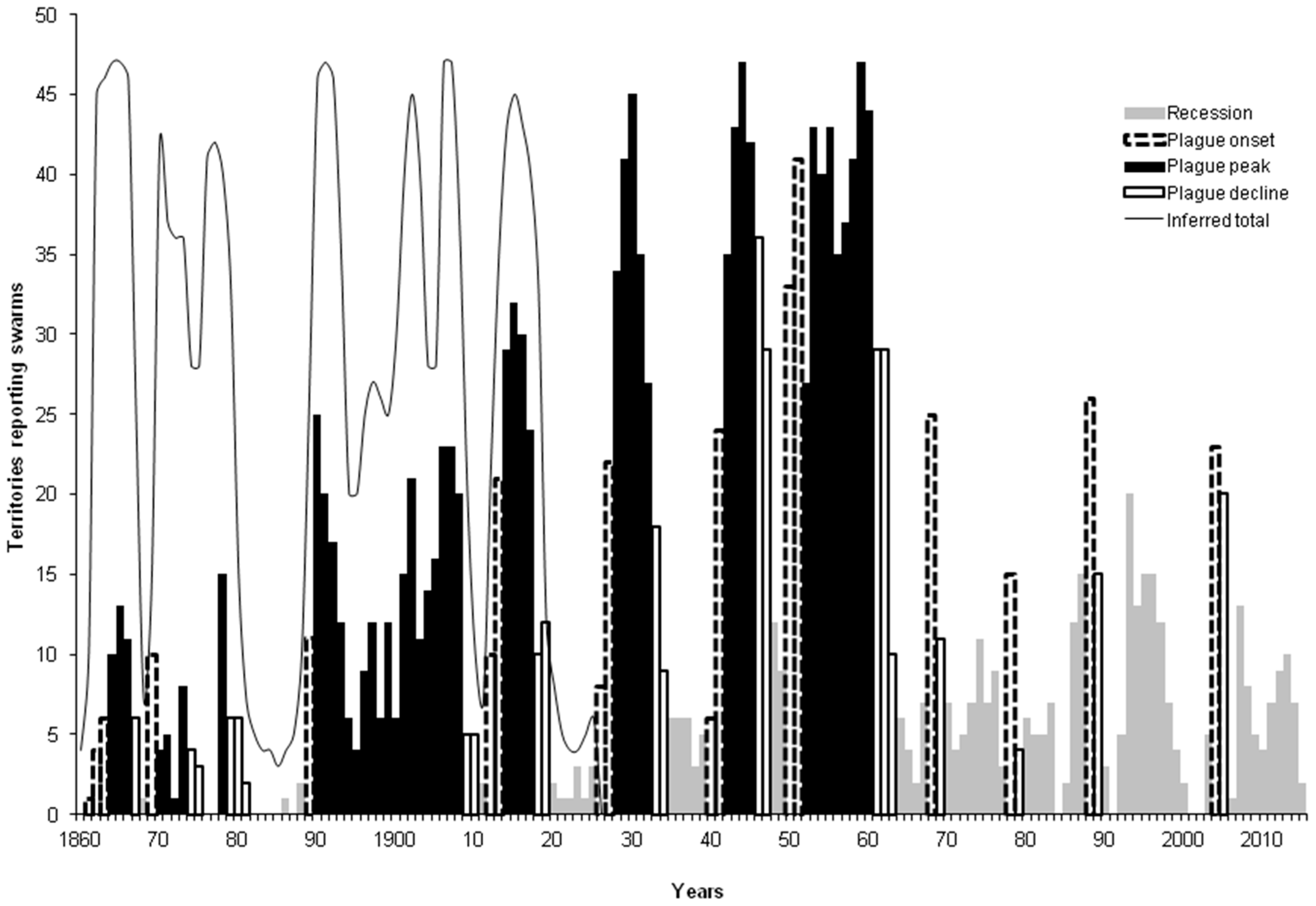
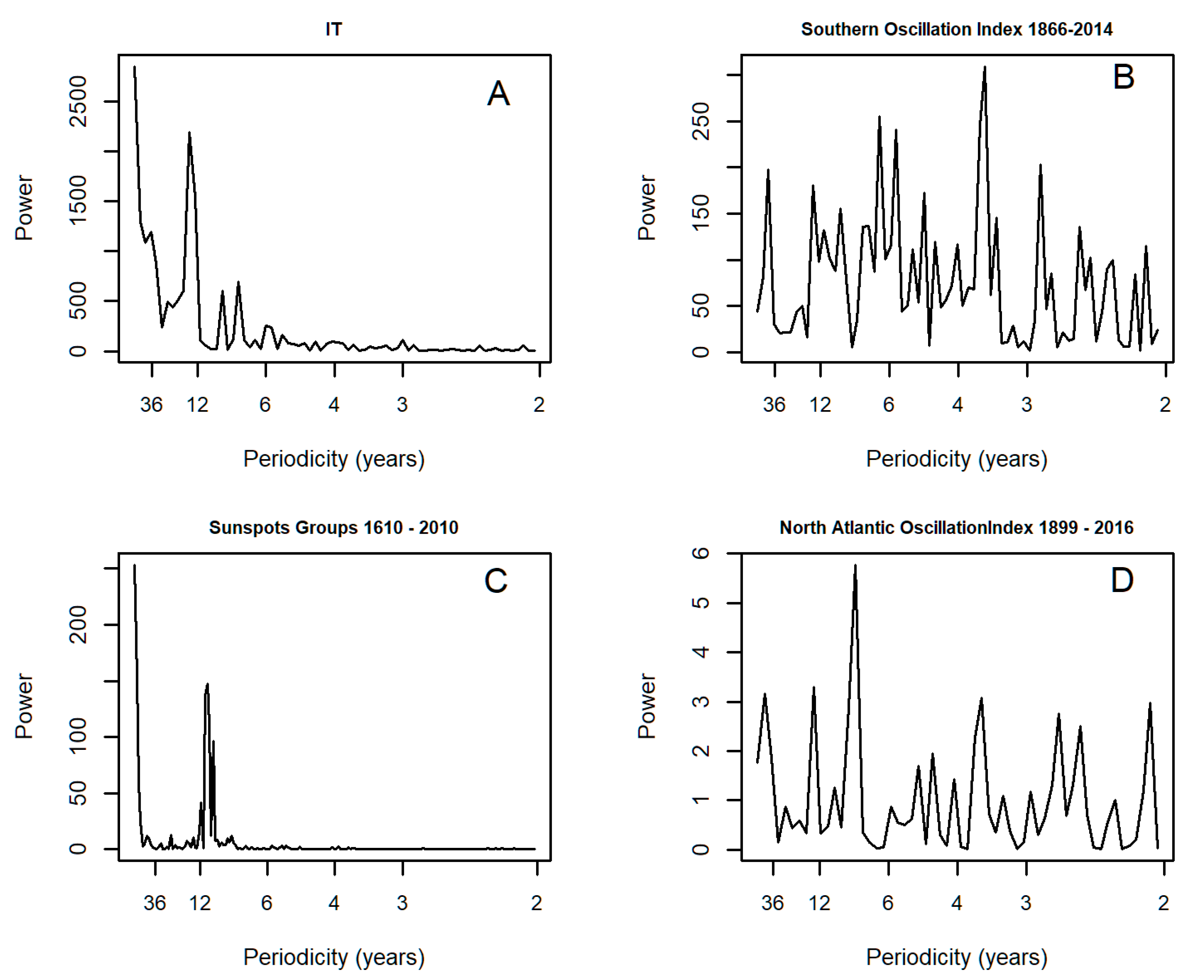
3.2. Spectral Analysis: Numbers of Territories Infested with Desert Locust Swarms, 1866–2010

Figure 2 shows the results of spectral analyses of the inferred Desert Locust series (IT), the sunspot groups and the SOI for the 1866 to 2010 data (truncated from 2014 as the available sunspot groups data only extend to 2010). For the Desert Locusts (1866 to 2014) there was a significant peak at a periodicity of 13.5 years (p = 0.02; based on the OUSS test) and another at a periodicity of 7.5 years (p = 0.02). The sunspot groups show a strong peak corresponding to a periodicity of 11.19 years (p < 0.0001). The SOI has a series of peaks at various periodicities but even the highest at a periodicity of 3.5 years was not significant (p = 0.62). The strongest peak in the annual NAO data for the 1899–2016 period was at a periodicity of 7.9 years, but this was only just significant with the OUSS test (p = 0.05).

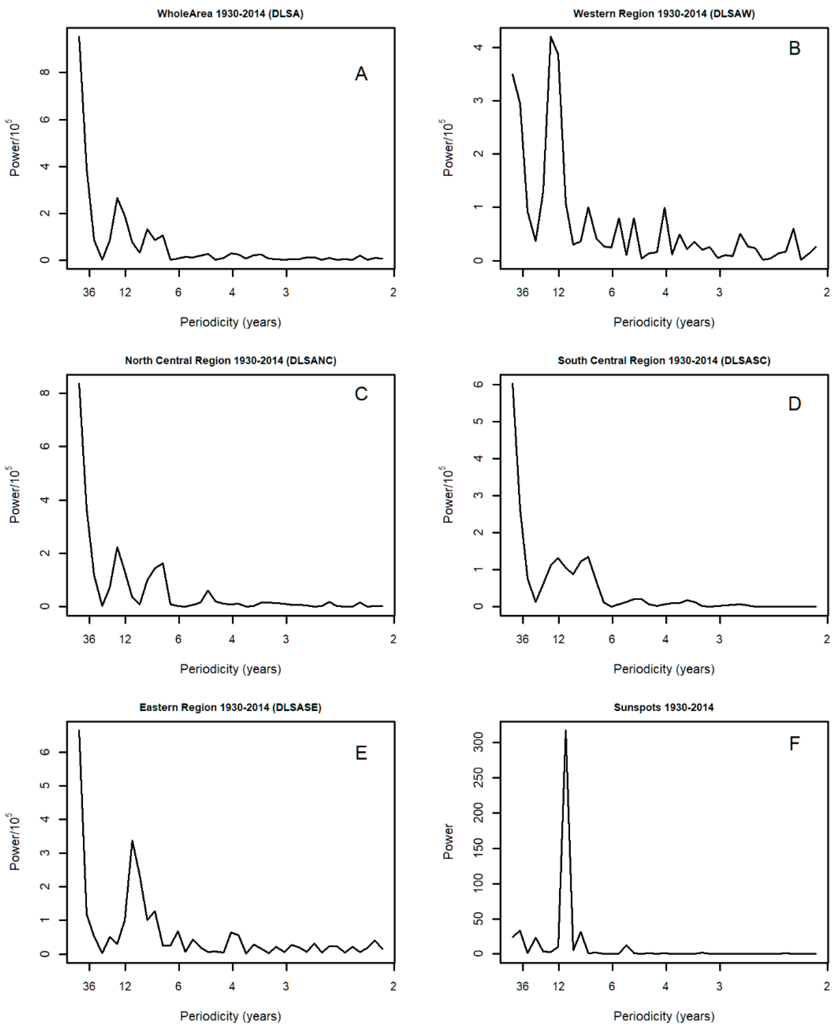
3.3. Spectral Analysis: Numbers of 1° Grid Squares Infested with Desert Locust Swarms, 1930–2014

Figure 3 shows the results of spectral analyses of the 1° grid square locust data total and according to region, together with the sunspot groups data for the shorter period (1930–2010). All of the locust series, analysed up to 2014 inclusive, show peaks for periodicities between 7 and 14 years. The peaks for the whole area’s data and for the Western and North Central regions corresponding to periodicities of 14 years are not significant with the OUSS test (p = 0.61) but are significantly different from white noise (p = 0.02). However, the peak corresponding to a periodicity of 7 years in the North Central Region’s data is significant with the OUSS test (p = 0.04). The highest peak in the Eastern region data corresponds to a periodicity of 10.6 years, not significant with the OUSS test (p = 0.2) but significantly different from white noise (p = 0.01). This peak is similar to the sunspot groups’ peak for this shorter series (1930–2010) which has a periodicity of 10.12 years, which is highly significant (OUSS test, p < 0.0001). Thus, although many of the peaks in the 1° grid square data are not significant with the OUSS test they do correspond in range with those for the longer IT series (see Section 3.2. above) which are significant at periodicities of about 7 and 14 years. No significant peaks were found by spectral analysis of the SOI data for 1930–2014.

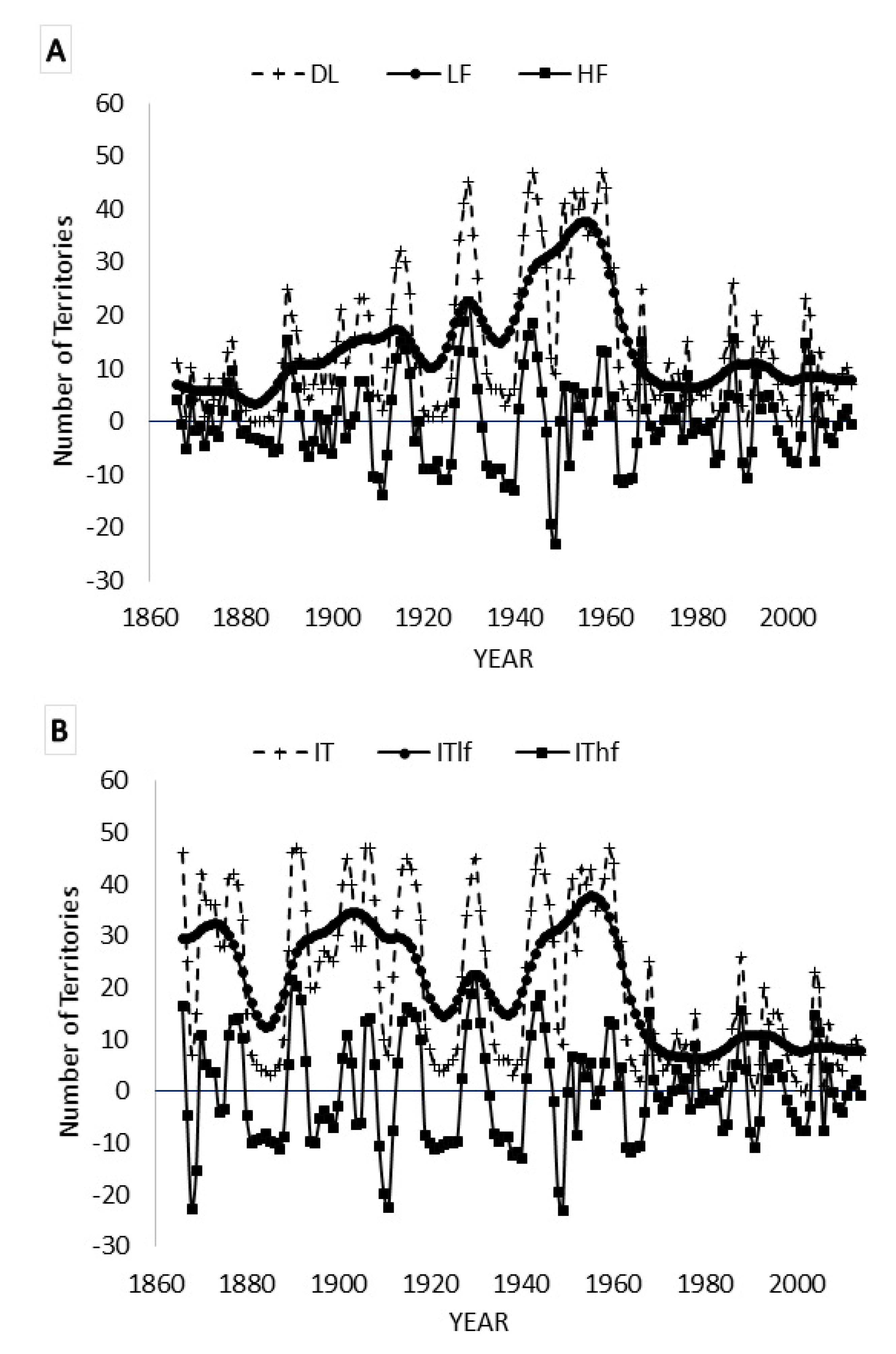
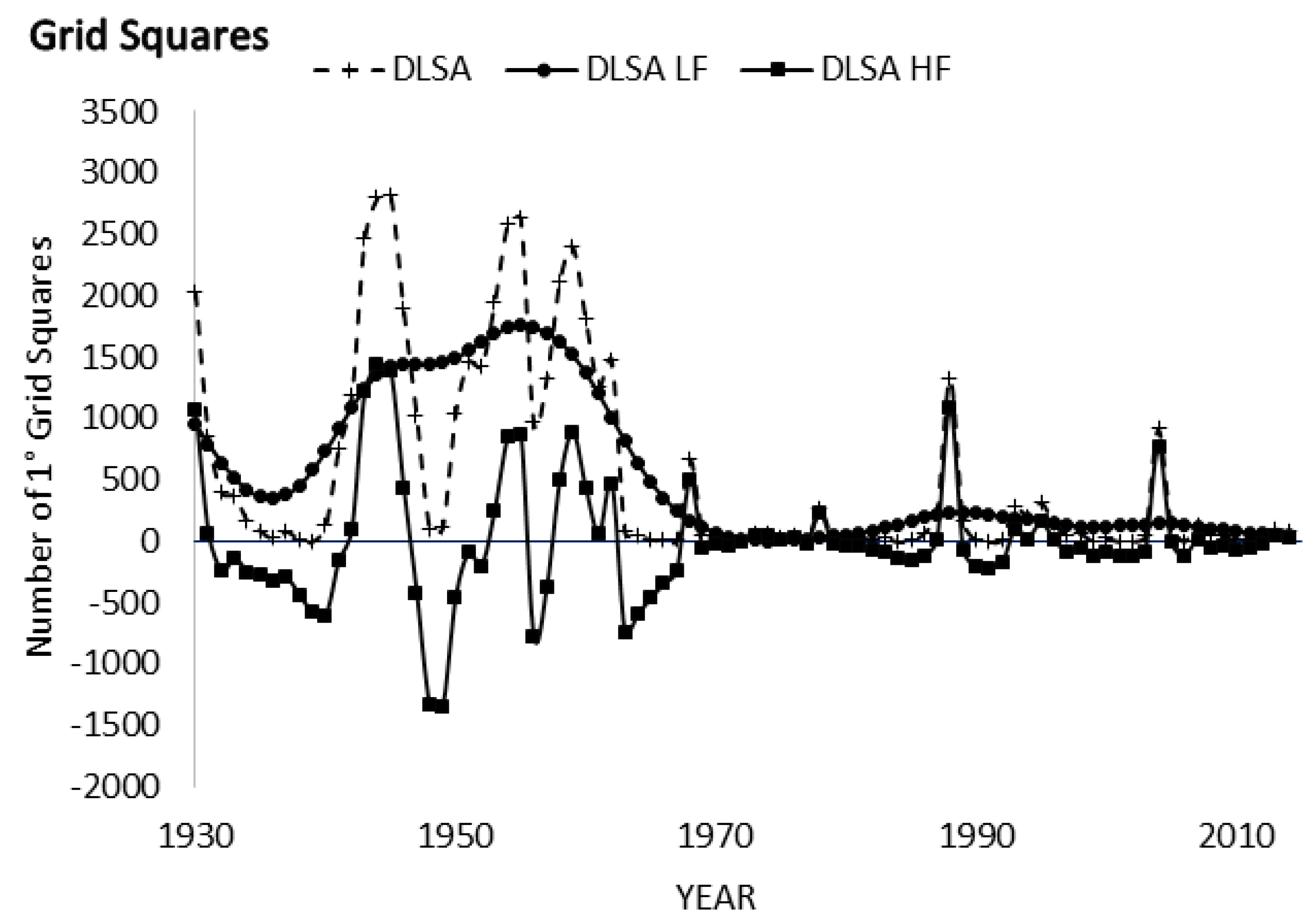
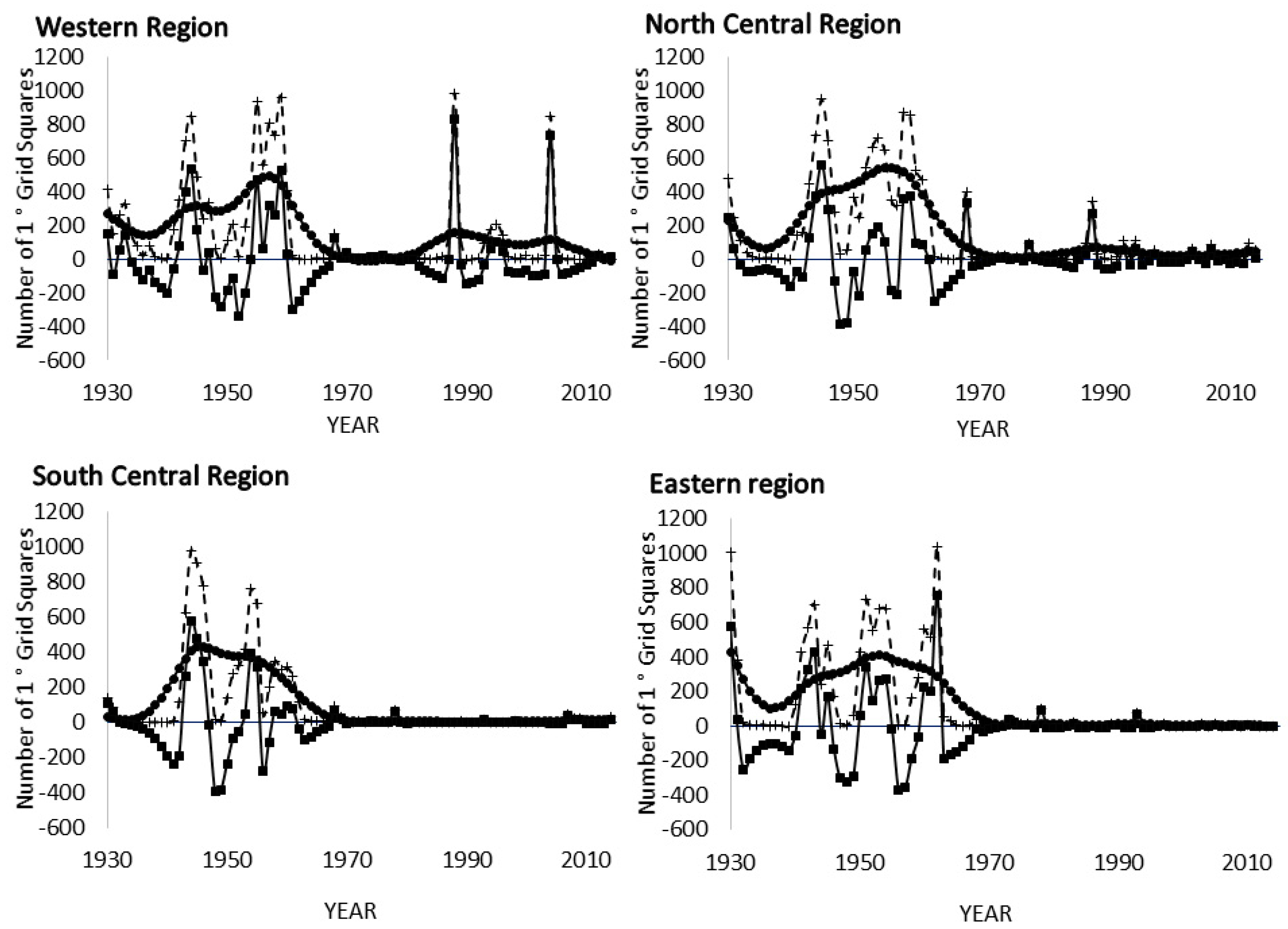
3.4. Kalman Filtering

Figure 4 shows the inferred numbers of territories series (IT) split into high and low frequency (ITlf) components by Kalman filtering and Figure 5 shows the SOI and NAO and their low and high frequency Kalman-filtered series. Figure 6 shows the numbers of 1° grid squares infested with swarms of Desert Locusts from 1930 to 2014 and the results of Kalman filtering and Figure 7 show the data arranged according to region.

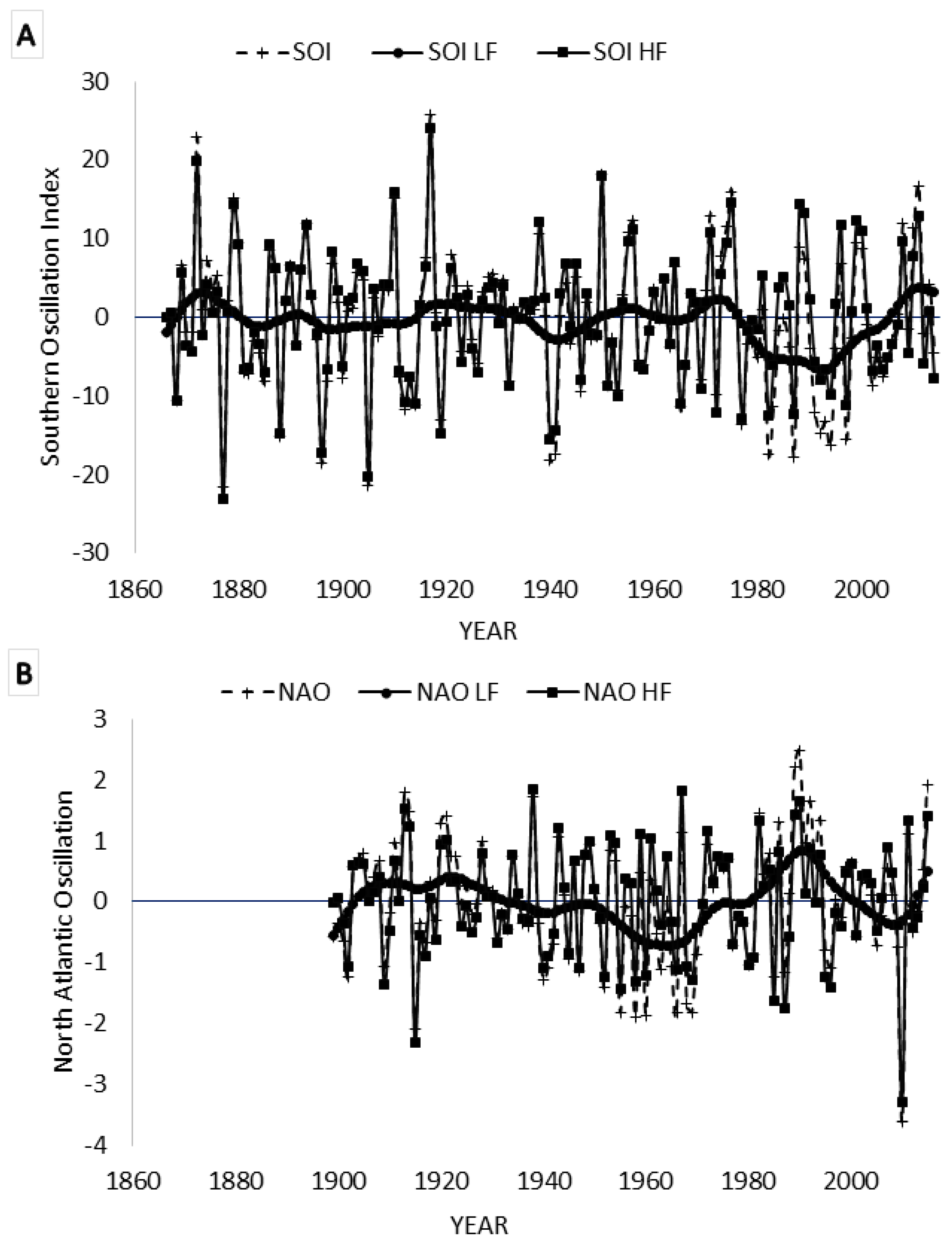
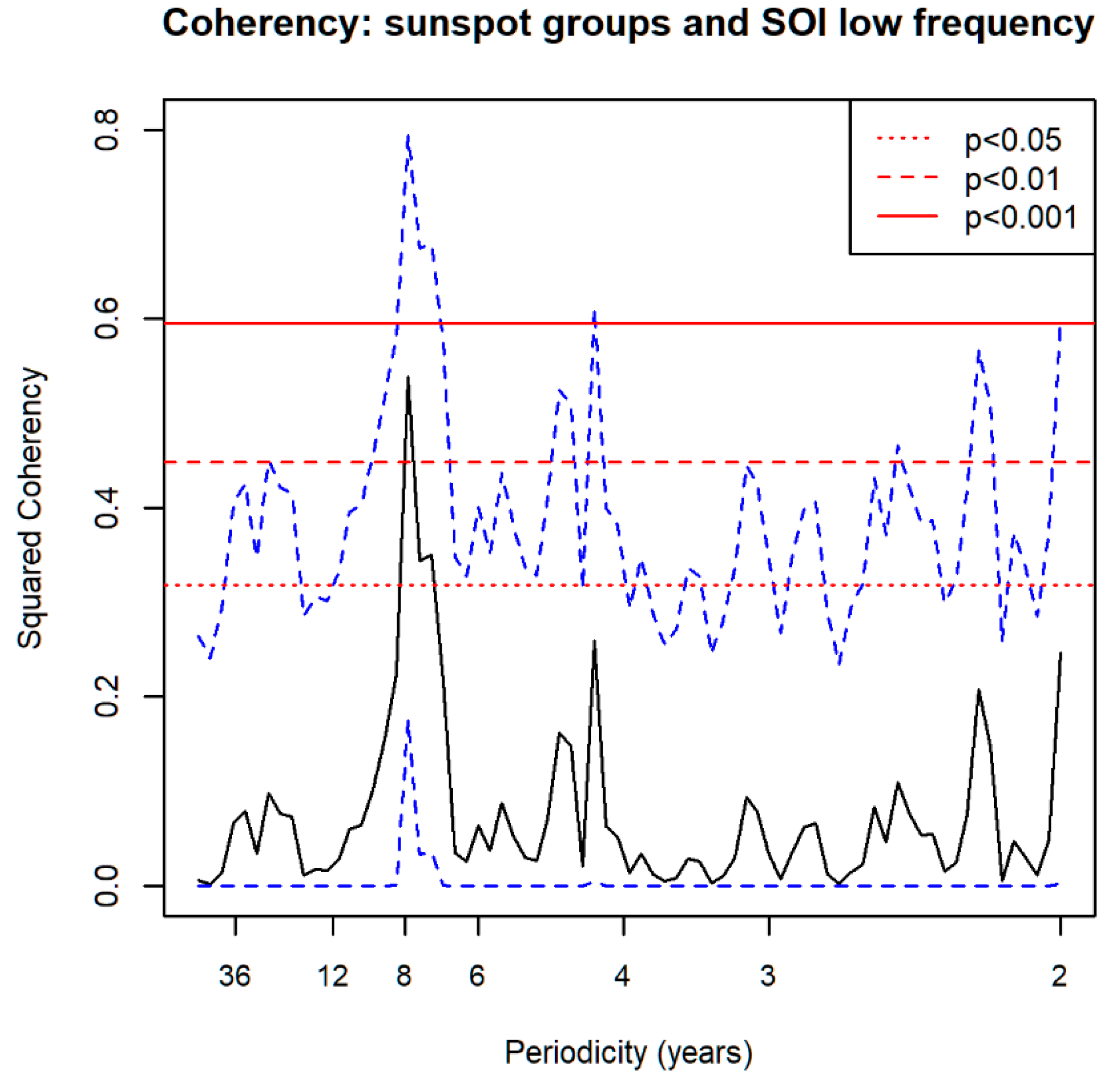
3.5. Spectral Coherence: Sunspots and Oceanic Systems

Table 2. Spectral coherence and convergent cross mapping CCM results between sunspot groups and oceanic indices. For spectral coherence significant coherent frequencies are denoted * for p < 0.05; ** for p < 0.01; *** for p < 0.001. Frequencies common to at least two pairs of time series in a row are highlighted in bold. NAO = North Atlantic Oscillation; NAOlf = low frequency component of NAO; IOD = Indian Ocean Dipole; SOI = Southern Oscillation Index; SOIlf = low frequency component of SOI.

		Time Series 2 (Response)
	NAO	NAOlf	IOD	SOI	SOIlf
Time Series 1 (Driver)
Spectral Coherence
Sunspot Groups	4.05 **	4.05 ***, 5.79 *	4.50 *, 2.37 **	NS	7.89 **
Convergence Cross Mapping
Sunspot Groups	NS	p < 0.0001	NS	NS	p = 0.04

presents results of spectral coherence tests for the sunspot groups data and various oceanic indices. Although the coherence between the sunspots and the unfiltered SOI is not significant there is a significant result (p < 0.01) for the sunspots and the low frequency SOI data at cycles of 7.89 years (Figure 8). There are also significant coherences between the sunspot groups and both the NAO and the low frequency component of the NAO at cycles of 4.05 years and with the IOD at 4.5 years.

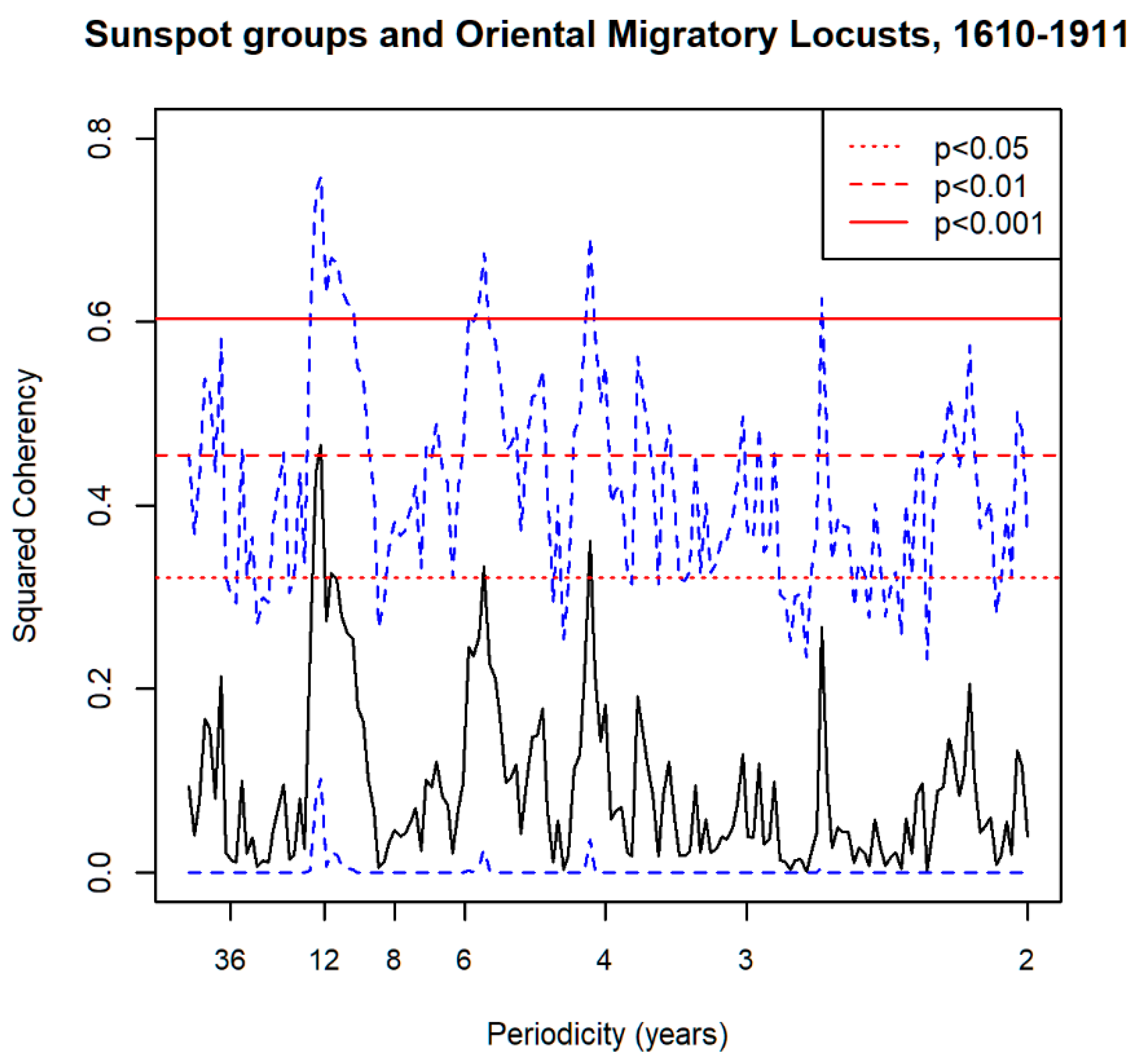
3.6. Spectral Coherence: Oriental Migratory Locusts

Significant spectral coherence was found between the 1610–1911 series of sunspot groups and the Oriental Migratory Locusts, with the main peak at 12.3 years (p < 0.01) and subsidiary peaks at 11.4, 5.6 and 4.2 years (all p < 0.05, Figure 9).

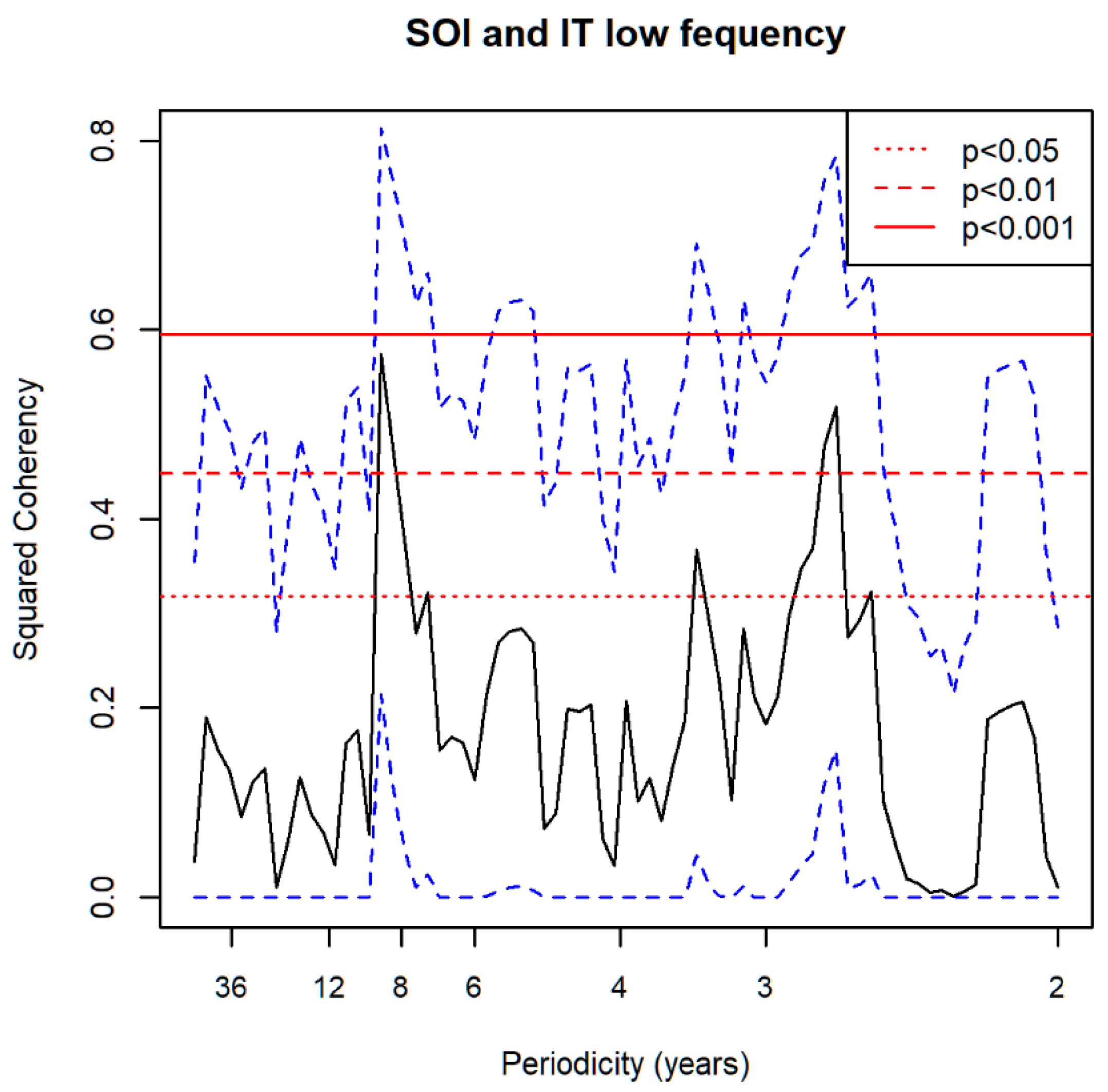
3.7. Spectral Coherence: Numbers of Territories Infested with Desert Locust Swarms, 1866–2014 (1866 to 2010 for Sunspot Groups Data)

Table 3. Spectral coherence results between Desert Locust time series and oceanic indices and sunspots. All statistically significant values of coherent cycle lengths are presented. Significant results are denoted * for p < 0.05; ** for p < 0.01; *** for p < 0.001. IT = Inferred Desert Locust series (1866–2014 [or 2010 for link with sunspots]); ITlf = low frequency component of IT; DLSA = 1° gridded data (1930–2014); DLSAlf = low frequency component of DLSA, followed by the same for regional data (W = West; NC = North Central; SC = South Central; E = East). SOI = Southern Oscillation Index; NAO = North Atlantic Oscillation; IOD = Indian Ocean Dipole; NAOlf = low frequency component of NAO, followed by seasonal data. Frequencies common to at least two pairs of time series in a row are highlighted in bold.

			Time Series 2 (Response)
	IT	ITlf	DLSA	DLSAlf	DLSAWlf	DLSANClf	DLSASClf	DLSAElf
Time Series 1 (Potential Driver)
Sunspot groups	22.86 *, 2.32 **	7.14 *, 2.27 *	6.23 *	6.75 ***, 4.26*	6.75 *	6.75 **, 4.26 *	6.75 *	6.75 ***
SOI	8.82 **, 7.89 *, 4.29 *, 3.95 *, 2.68 ***, 2.54 **	8.83 **, 8.33 *, 3.41 *, 2.67 **, 2.54 *	NS	NS	NS	NS	NS	NS
SOIlf	10.71 *, 7.14 *, 5.17 *, 4.0 **, 3.75 *, 2.68 **, 2.54 **	15.0 *, 10.71 *, 8.82 ***, 7.14 **, 5.0*, 3.41 *, 3.09 * 2.68 **, 2.54 *	NS	6.43 **, 4.74 ***, 2.90 *	12.86 *, 6.92 ***, 4.09 **, 3.21 **	6.42 *, 5.0 ***, 3.10 *, 2.90 *	5.0 ***, 3.21 *, 2.90 *	6.43 **, 5.0 **, 2.90 *, 2.14 **
NAO	2.10 **	3.24 *, 2.10 **	NS	4.5 *	4.5 *	4.5 *, 4.09 *, 3.75 *, 3.33 *	NS	NS
NAOlf	9.23 ***, 6.32 ***, 2.10 ***	60.0 *, 17.14 **, 9.23 ***, 6.0 **, 3.16 *, 2.10 ***	NS	15.0 *, 8.18 ***, 4.5 ***	18.0 *, 8.18 *, 6.0 *, 4.74 **	15.0 *, 8.18 ***, 4.5 *	8.18 ***, 5.29 *, 4.74 *, 4.5 *, 2.19 *, 2.0 *	20 *, 7.5 *, 6.92 **, 4.5 ***, 3.12 *, 2.18 *
NAODJFlf (winter)	9.23 *, 6.0 **	17.14 ***, 9.23 ***, 6.0 ***, 5.22 *	NS	15.0 *, 8.18 ***, 4.5 ***	15.0 *, 8.18 *, 6.0 *, 4.74 **, 4.29 *	15.0 *, 8.18 *** 4.74 ***	8.18 ***, 5.29 *, 4.74 *	15.0 *, 6.92 **, 4.5 ***, 3.21 *, 2.90 *
NAOMAMlf (spring)	9.23 *, 6.0 *	9.23 ***, 6.0 ***, 3.24 *	3.21*	15.0 *, 10.0 *, 6.43 *, 4.74 ***	18.0 *, 9.0 **, 6.43 ***, 4.5 *	15.0 **, 10.0 *, 6.43 **, 4.74 ***	15.0 **, 9.0 *, 7.5 *, 4.74 ***	18.0 **, 6.43 ***, 4.74 ***, 2.81 *
NAOJJAlf (summer)	20 *,10 *, 6.67 *, 4.8 *	20 **, 13.33 **, 10 **, 8 **, 6.67 **, 4.8 **, 3.53 ***	NS	30.0 **, 15.0 **, 9.0 ***, 6.43 *, 5.29 ***, 4.28 *, 3.10 *	30.0 **, 15.0 **, 11.25 **, 9.0*, 6.92 **, 5.29 *, 4.29 **, 3.21 *, 2.09 *	15.0 **, 9.0 ***, 5.29 **	30.0 **, 15.0 **, 9.0 ***, 5.29 ***, 3.21 **	15.0 **, 9.0 **, 6.0 **, 5.29 **, 4.29 ***, 3.10 **, 2.09 **
NAOSONlf (autumn)	9.23 *, 3.64 *, 2.40 **	15.0 *, 9.23 ***, 6.0 *, 4.8 *, 3.33 * 2.40 ***	9.0 *, 5.62 *	9.0 ***, 6.43 **, 5.0 **	12.86 *, 9.0 ***, 6.92 ***, 3.33 *	9.0 ***, 6.43 **, 5.0 ***	11.25 ***, 9.0 ***, 5.0 ***	9.0 *, 6.43 ***, 5.0 *
IOD (Mean DMI)	12.27 *, 3.21 *	3.37 **	NS	7.20 *	NS	NS	NS	NS

shows the results of spectral coherence tests for different potential drivers and each of the Desert Locust series. There were significant coherences between all potential drivers tested and both IT (inferred Desert Locust series) and ITlf (low frequency (lf) component of IT) at many different frequencies, but these significant frequencies differed amongst both drivers and locust series making interpretation difficult. Furthermore, these cycle lengths differed slightly as the Daniell smoothing factor varied (e.g., by increasing it from 4 to 7), although the same combinations of drivers and locust series were still found to be significant. Nevertheless, given the results of spectral analyses indicative of cycles of between 7 and 14 years, coherences within this range may be the most informative. Those of interest include the link between the sunspot groups and the ITlf at 7.14 years (p< 0.05), a frequency recurring for the effects of the low frequency component of the SOI (SOIlf) on both IT (p < 0.05) and ITlf (p < 0.01). The coherences between the SOI and both IT and ITlf at 8.8 years (both p < 0.01; Figure 10), a result repeated for the coherence between SOIlf and ITlf (p < 0.001), are also of interest. In the table, frequencies repeated along a row have been highlighted in bold; these include the coherences between SOIlf and both IT (p < 0.05) and ITlf (p < 0.01) at 10.7 years. The low frequency component of NAO (NAOlf) has highly significant (p < 0.001) coherences with IT and ITlf at 9.23 years, a frequency repeated for both IT and ITlf with all of the seasonal versions of NAOlf except that for June–August.

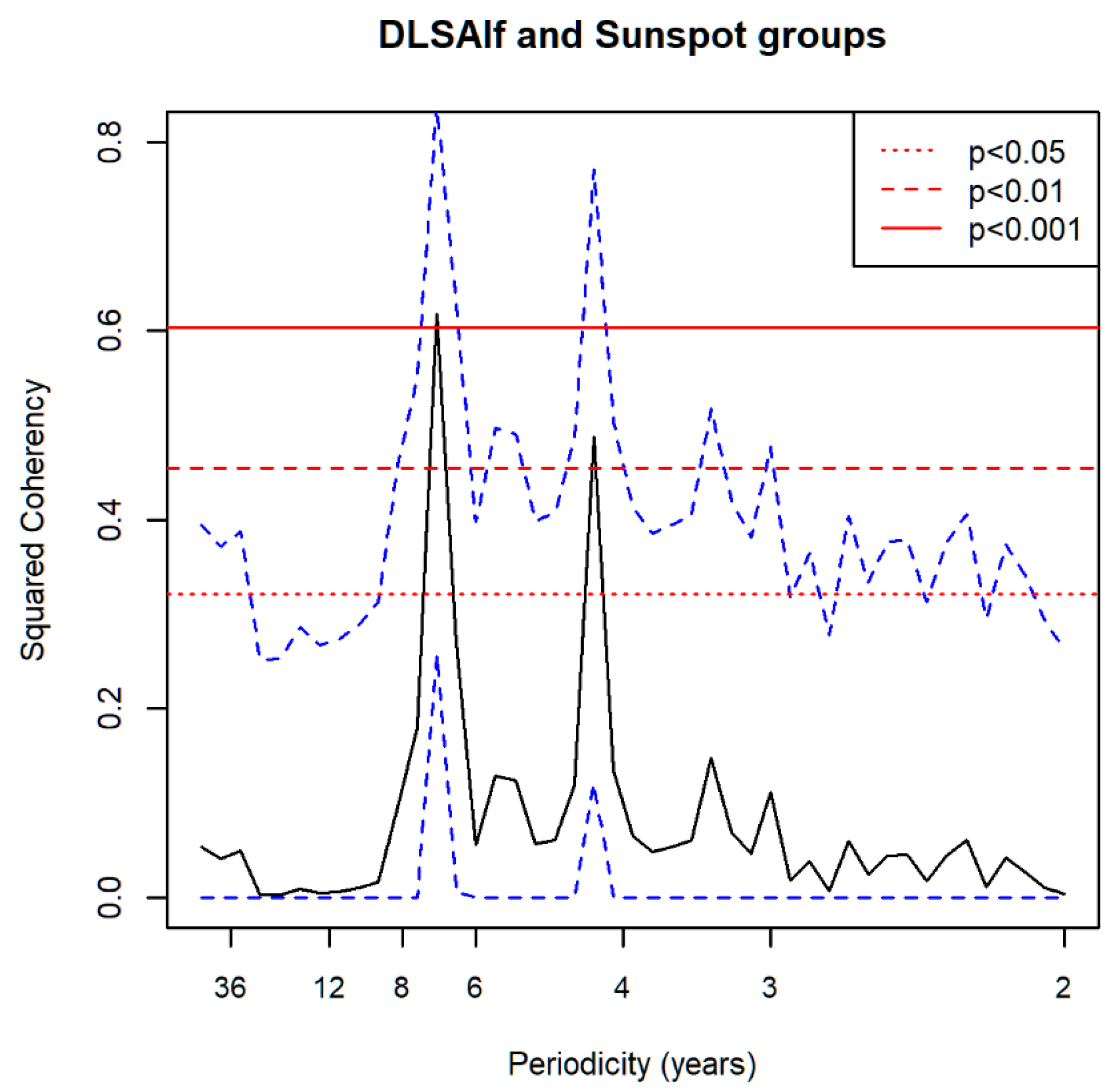
3.8. Spectral Coherence: Numbers of 1° Grid Squares Infested with Desert Locust Swarms, 1930–2014

The sunspot groups have significant spectral coherence with the unfiltered total number of 1° grid squares infested with desert locusts (DLSA) series at a frequency of 6.23 years (p < 0.05) but a consistent coherence at 6.75 years for all of the low frequency gridded data series regardless of region (p < 0.001 for DLSAlf (Figure 11) and DLSAElf, p < 0.01 for DLSANClf and p < 0.05 for DLSAWlf and DLSASClf).

No significant spectral coherence was detected between the SOI and the DLSA series (Table 3), but the SOIlf had coherences with all low frequency gridded data sets with a frequency of 6.4 years recurring in DLSAlf and the South Central and Eastern regions.

The unfiltered NAO data showed consistent coherence at 4.5 years with DLSAlf and the low frequency regional data sets for the Western and North Central regions (all p < 0.05). The NAOlf and the December to January version of it were consistently coherent with all low frequency versions of the locust gridded data at 8.18 years, except in the Eastern region. The link at 9 years between the September-November version of the NAOlf and all versions of the locust gridded data, which also tallied with the 9.2 years noted for the same potential driver with the IT and the ITlf, was also remarkable.

The IOD showed weak coherence with DLSAlf at 7.2 years (p < 0.05), but not with the regional data, but as this oceanic system is linearly correlated with the SOI (p < 0.001) it was not surprising that results were similar for both systems.

3.9. Convergent Cross Mapping: Sunspot Groups and Oceanic Systems

Although there was no evidence of a causal relationship between the sunspot groups and the ocean oscillation systems when unfiltered data were used, significant causal relationships were found between sunspot groups and the low frequency components of both the SOI (p = 0.04) and the NAO (p < 0.0001), which is consistent with the spectral coherence results (Table 2).

3.10. Convergent Cross Mapping: Oriental Migratory Locusts

Although there was no evidence of a causal relationship between the sunspot groups and the unfiltered Oriental Migratory Locust data, a significant effect of the sunspot groups causing its low frequency was detected (p = 0.001) but this result is invalid as the reverse, impossible, result (OML causing sunspots) was also significant (p < 0.04).

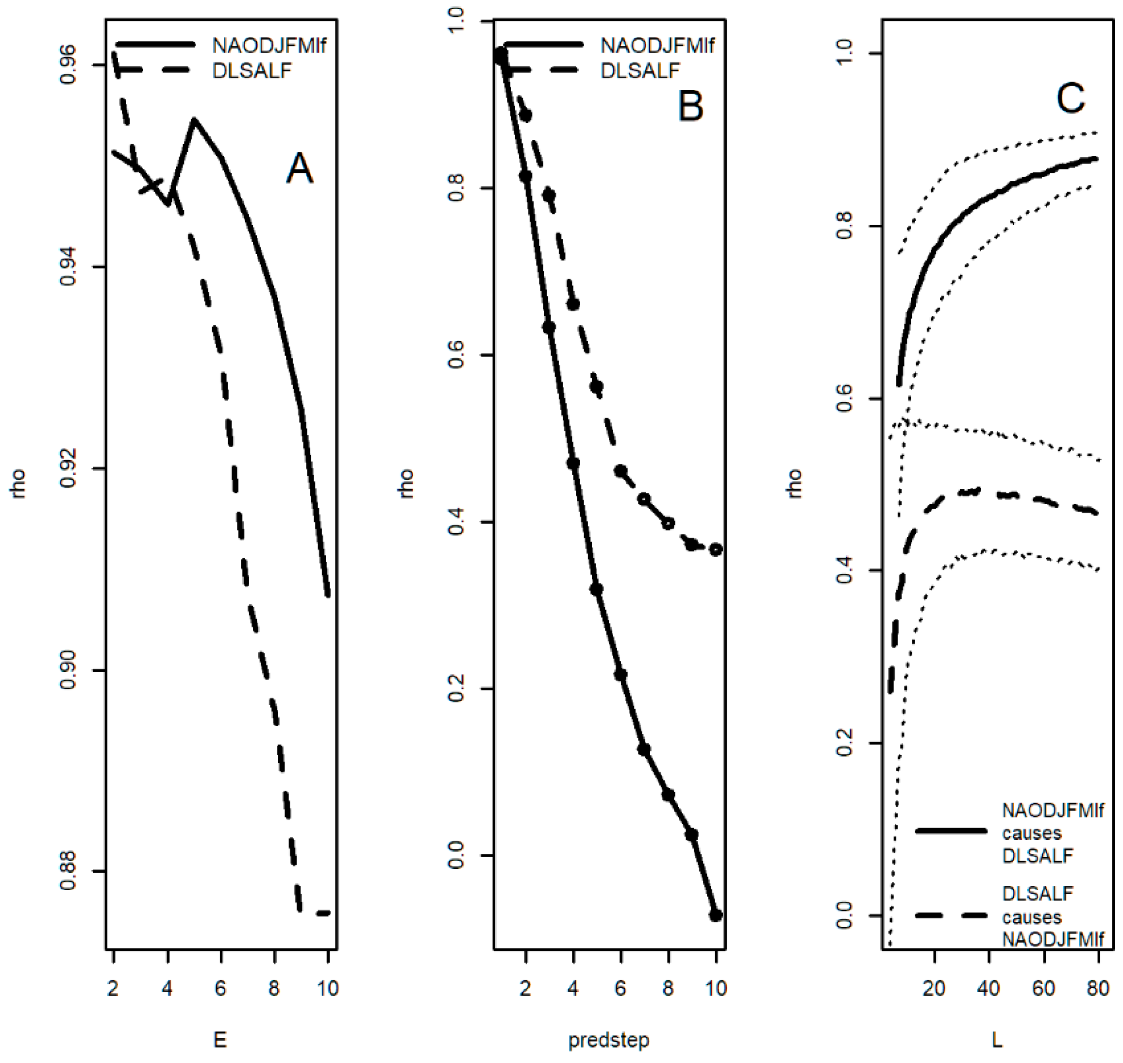
3.11. Convergent Cross Mapping (CCM): Desert Locusts

Remarkably, CCMs gave strong evidence for sunspot groups causing changes in Desert Locust abundance as measured in all of the locust series (p < 0.0001 in every case;

Table 4. Results of analyses using CCM tests of causality of various time series (drivers) causing the low frequency inferred Desert Locust series 1866–2014 (ITlf) and the gridded Desert Locust series (1930–2014). p values given if relationships statistically significant (NS = not significant). Note that the results for the unfiltered sunspot groups data (1866–2010) reveals significance for all relationships with the gridded Desert Locust data. DLSA = 1° gridded data (1930–2014); DLSAlf = low frequency component of DLSA, followed by the same for regional data (W = West; NC = North Central; SC = South Central; E = East). SOI = Southern Oscillation Index; NAO = North Atlantic Oscillation; NAOlf = low frequency component of NAO, followed by seasonal data.

			Time Series 2 (Response)
	ITlf	DLSA	DLSAlf	DLSAWlf	DLSANClf	DLSASClf	DLSAElf
Time Series 1 (Driver)
Sunspot Groups	<0.0001	<0.0001	<0.0001	<0.0001	<0.0001	<0.0001	<0.0001
SOIlf	<0.005	NS	<0.0001	NS	NS	0.001	0.002
NAOlf	NS	NS	<0.0001	0.001	<0.005	<0.0001	0.003
NAODJFlf	NS	NS	0.034	NS	NS	0.0007	NS
NAOMAMlf	<0.0001	NS	<0.0001	NS	0.009	<0.0001	0.0007
NAOJJAlf	0.01	NS	0.038	NS	0.021	<0.005	<0.0001
NAOSONlf	<0.0001	NS	0.048	0.05	<0.003	<0.003	NS
NAODJFMlf	NS	NS	0.0007	0.002	0.004	<0.0001	<0.003

; Figure 12), except for the unfiltered data of the inferred series (IT). No potential driver was found to be causing changes in the IT but, in addition to the sunspot groups result, there was also evidence of the ITlf being driven by the SOIlf (p < 0.005), and by the low frequency versions of the NAO for March to May (p < 0.0001), June to August (p < 0.01) and September to November (p < 0.0001).

The low frequency component of the Kalman-filtered numbers of 1° grid squares infested with Desert Locust swarms for the 1930 to 2014 period (DLSAlf) was also found to be causally linked to the low frequency component of the SOI (SOIlf, p < 0.0001). This relationship also held true when the SOIlf data were analysed at the regional level for the South Central (p < 0.001) and Eastern regions (p = 0.002), but not for the North Central and Western regions.

The low frequency component of the NAO for the 1930–2014 period was consistently shown by CCM to drive the low frequency components of the gridded data (DLSAlf, p < 0.0001; DLSAWlf, p < 0.001; DLSANClf, p < 0.005; DLSASClf, p < 0.0001; DLSAElf p < 0.003). These results were to a large degree matched when the seasonal versions of the NAOlf data were used, with strong evidence (p < 0.01) of a causal link between the December to March version and all of the low frequency gridded data sets, including the entire (whole year, all regions aggregated) series (DLSAlf) (Figure 13).

4. Discussion

The analyses described above have provided evidence for causal links between the solar cycle, measured by numbers of sunspot groups, and low frequency components of the NAO and the SOI (Table 2) and between both unfiltered NAO and SOI data and their low frequency components with indices of population variation in both Desert Locusts (Table 3 and Table 4) and Oriental Migratory Locusts (Section 3.6 and Section 3.10). From these results it might appear that the solar activity is driving the oceanic systems and that these are, in turn, driving the locusts. However, such an explanation is simplistic since the links between the sunspot data and the oceanic systems are weak and the cycle lengths detected are not consistent with each other. Indeed, a recent study failed to find a significant link between solar activity and the NAO [45], so our finding of spectral coherence between sunspot group numbers and both the unfiltered series and the low frequency components of the NAO (and with the LF SOI) may be of more interest to climatologists than to entomologists. Nevertheless, what is clear from our results is that there are causal relationships between solar activity and locusts, but this may not necessarily be via the oceanic systems, directly, but perhaps via some other means whereby the sun influences weather patterns.

We have also demonstrated for the first time that there is cyclicity in the dynamics of Desert Locust populations (Section 3.2). The latter result contrasts with the conclusion of Waloff [25] that there are no regular cycles in Desert Locust outbreaks, but lends support to the findings of Cheke and Holt [9] that there were was some evidence for 7 and 13 year cycles in a series of data up to 1990, although these were not statistically significant. Spectral analysis confirmed the existence of a statistically significant 13.5 year cycle, a near harmonic of the similarly significant peak at 7.5 years, in the 1866 to 2015 inferred series of numbers of territories infested with Desert Locust swarms. Similar periodicities were evident in the shorter 1930–2014 1° grid square data sets but these were not significant according to the stringent OUSS test, although they were significantly different from white noise according to the Kolmogorov-Smirnov test. Although Waloff and Green [46] argued that there was no evidence of periodicity in locust plagues, their data on the frequency distribution of intervals between onsets of successive regional plagues were highest (9 instances) at 5–7 years and 14–16 years (8 instances). With the above evidence for cycles of 7.5 and 13.5 years, it is of considerable interest that the significant and most consistent coherent frequencies between different drivers and the locust dynamics reported in Table 3 include 8.8 (SOI) and range from 6.23 to 7.14 (sunspot groups) and from 8.2 to 15 (low frequency NAO). A possible explanation for some of these results, as far as the sunspot groups is concerned given their well-known approximately 11 year cycle (confirmed here, Figure 2c), could be forthcoming if there is a certain low value of solar activity responsible for triggering appropriate meteorological events conducive to locusts. Such a value would be reached both when the solar activity is rising towards its peak and when it is descending to a trough and, depending on the magnitude of such a certain value in relation to the period of the cycle, the interval between these events could be about every 6–8 years.

Although there were no significant cycles detected by spectral analysis of the Oriental Migratory Locust data, there was significant spectral coherence between the sunspot groups and the Oriental Migratory locusts at 12.3 years, evidence of a link between them. In this context it is of interest that statistically significant (p < 0.05) peaks at 17.3, 3.7 and 2.9 years have been reported previously for the Brown Locust [14].

The different values for the spectral coherences associated with different drivers (Table 3) are difficult to interpret and may reflect inaccuracies resulting from the methods used (e.g., see Section 3.7. for comment on effects of varying the Daniell smoothing span in spectral coherence) but it needs to be borne in mind that Desert Locust outbreaks do not spring from a single source outbreak area, but from a variety of gregarisation zones located in each of the four regions (Western, North Central, South Central and Eastern, see maps in [26,47]) within a huge 10,000 km wide geographical area from West Africa to India. Therefore, it is to be expected that different oceanic drivers or their seasonal variants could be responsible for causing outbreaks in different regions. Thus, Waloff [25] reported three upsurges originating in the Western region, three in the North Central region, one in the South Central region and four in the Eastern region. Therefore, different oceanic drivers or seasonal variants of them could be responsible for causing outbreaks in different regions at different frequencies, as suggested by some of the results in Table 3. In addition, once an outbreak has started the locusts will often move out of their region of origin into another region and flourish there, resulting in a detectable signal from an oceanic driver being linked to the second rather than the first region. Such considerations may explain why the low frequency series of the NAO for September-November shows consistent coherence with all of the Desert Locust series tested (Table 3) at nine year intervals, whereas they might be expected to be most influential on the Western or North Central regions. It should also be borne in mind that an increase in the low frequency component of the locust dynamics will not always be reflected in a corresponding high frequency increase if weather conditions or control activities curtail a locust upsurge.

Both conventional statistical methods and the convergent cross mapping revealed relations between the SOI and the Desert Locust time series. The results for the inferred series and the shorter 1° grid square series were not always consistent and there are some regional variations to be discussed below. The SOI has high values during cold La Niña conditions and low values during warm El Niño circumstances (See https://www.ncdc.noaa.gov/teleconnections/enso/indicators/soi/). The short-term high frequency components of Brown Locust numbers have previously been found to be high during La Niña periods [14], but here we have concentrated on the long-term low frequency components. The rationale for the association is that there will be higher rainfall, essential for locust success, in many of the Desert Locust outbreak areas when La Niña cold conditions lead to more rain than the quantities that fall during the warm El Niño periods. This is supported by the CCM analyses suggesting causal links with the low frequency SOI driving the low frequency DLSA data set for the total number of infested 1° grid squares. However, at the regional level the links only held for the low frequency SOI with the South Central and Eastern regions’ locust data, confirming our hypothesis that there are regional variations.

The NAO is a key factor that is responsible for inter-annual variability over extensive geographical zones, but especially of the north African climate [48]. When the NAO is low in winter, the north African climate tends to be warm and wet, and there is an inverse relation between the December to February NAO and November to April rainfall over Morocco [49]. Across western Africa, annual variations in seasonal climatic conditions are determined primarily by the Atlantic Ocean, although the rest of the world’s oceans also play important roles (http://www.ipcc.ch/ipccreports/tar/wg2/index.php?idp=380). The temperature in the Sahara is affected by the NAO, with warmer winter temperatures during negative NAO events and cooler winters with more frosts when the NAO is positive [30]. Thus, the finding that the low frequency DJFM NAO data have the strongest causal links with the low frequency locust data according to the CCM tests (Table 4) is consistent with such NAO variability. Indeed, as already mentioned above, the NAO has correlations in DJFM that reach across Europe into the Middle East and Asia (see Figure 1 of [30]).

Inspection of Figure 1 reveals that, until the current upsurge began in 2018, in recent years there has been reduced locust activity. An exception was the Western region, where many upsurges begin. It is likely that the lack of major plagues until very recently was attributable to modern control practices. However, it may also explain why some of the cycles and trends were not as clear in the 1930–2014 1° grid square series in comparison with the long 1866–2014 inferred territories series, but this could also be explained by the higher likelihood of any patterns in the data being demonstrated to be statistically significant as the number of observations increases [50].

Given the number of statistical tests carried out (Table 2, Table 3 and Table 4), it is likely that some statistically significant results could have been found by chance alone but there are sufficient consistencies in the results for us to consider that it is unlikely that they are spurious. For instance, many of the CCM results are consistent with the spectral coherence tests (e.g., for sunspot groups) and the evidence suggests that there are links between sunspots and the locusts, probably mediated by the influence of the sunspots on oceanic systems (Table 2 shows the low frequency SOI to be coherent at a frequency of 7.89 years with the sunspots), and hence through weather systems, although exactly how this is achieved remains unclear and requires further research. In addition, given the evidence for cyclicity in the sunspots and likely delays in a similar response in the insect dynamics, it is possible that with further research a method of forecasting long-term trends in Desert Locust outbreaks may become feasible to supplement the short term methods [12] currently in use. As emphasised in the Introduction, the analyses presented here sought trends for the long term dynamics and ultimate causative factors, with results suggesting recurrences every 7–15 years, whereas the proximate factor, rainfall, is linked to the short-term dynamics with lags of 4 to 12 months [10]. Future research will seek to use the results presented here to develop models capable of providing early warning forecasts, perhaps by developing models based on the techniques described by Ye et al. [43] and Chen et al. [44]. For this, it will be necessary to examine detailed effects of lags (all of the CCM results discussed here assumed that tau = 1) to devise predictive models that could be tested to see if they anticipate the Desert Locust outbreak that began in 2018 (incidentally during a solar minimum) and to test the hypothesis that some outbreaks are driven by the SOI and others by the NAO in relation to seasonal and geographic variations in rainfall and locust abundance.

5. Conclusions

Statistically significant cyclicity exists in the population dynamics of the Desert Locust Schistocerca gregaria at periods of 7.5 and 13.5 years, according to results of spectral analysis of the well-known inferred time series. Tests using the methods of spectral coherence and convergent cross mapping revealed statistically significant evidence that dynamics of both Desert Locusts and Oriental Migratory Locusts Locusta migratoria manilensis and, in particular their low frequency dynamics, are causally linked with numbers of sunspot groups. In addition, causal links were inferred between both the Southern Oscillation Index (SOI) and the North Atlantic Oscillation (NAO) and Desert Locust dynamics, with the NAO for December-March being most influential. Solar activity seems to play a role in driving locust abundance, but by exactly what means and the extent to which fluctuations in oceanic systems are determinants remains unclear, although weak causal links between the sunspots and both the SOI and the NAO were also found. Nevertheless, it is possible that further research on the phenomena identified may eventually enable better early warning forecasting of desert locust upsurges.

References

1. Cisse, S.; Ghaout, S.; Mazih, A.; Ebbe, M.A.O.B.; Piou, C. Effect of vegetation on density thresholds of adult desert locust gregarization from survey data in Mauritania. Entomol. Exp. Appl. 2013, 149, 159–165. [Google Scholar] [CrossRef]
2. Cisse, S.; Ghaout, S.; Mazih, A.; Ebbe, M.A.O.B.; Benahi, A.; Piou, C. Estimation of density threshold of gregarization of desert locust hoppers from field sampling in Mauritania. Entomol. Exp. Appl. 2015, 156, 136–148. [Google Scholar] [CrossRef]
3. Uvarov, B. Grasshoppers and Locusts. A Handbook of General Acridology; Cambridge University Press: Cambridge, UK, 1966; Volume 1. [Google Scholar]
4. Uvarov, B. Grasshoppers and Locusts. A Handbook of General Acridology; Centre for Overseas Pest Research: London, UK, 1977; Volume 2. [Google Scholar]
5. Simpson, S.J.; McCaffery, A.R.; Hägele, B.F. A behavioural analysis of phase change in the desert locust. Biol. Rev. Camb. Philos. Soc. 1999, 74, 461–480. [Google Scholar] [CrossRef]
6. Simpson, S.J.; Despland, E.; Hägele, B.F.; Dodgson, T. Gregarious behavior in desert locusts is evoked by touching their back legs. Proc. Natl. Acad. Sci. USA 2001, 98, 3895–3897. [Google Scholar] [CrossRef] [PubMed] [Green Version]
7. Desert Locust Guidelines, 2nd ed.; FAO: Rome, Italy, 2001.
8. Cullen, D.A.; Cease, A.J.; Latchininsky, A.V.; Ayali, A.; Berry, K.; Buhl, J.; De Keyser, R.; Foquet, B.; Hadrich, J.C.; Matheson, T.; et al. From molecules to management: Mechanisms and consequences of locust phase polyphenism. Adv. Insect Physiol. 2017, 53, 167–285. [Google Scholar] [CrossRef]
9. Cheke, R.A.; Holt, J. Complex dynamics of desert locust plagues. Ecol. Entomol. 1993, 18, 109–115. [Google Scholar] [CrossRef]
10. Tratalos, J.A.; Cheke, R.A.; Healey, R.; Stenseth, N.-C. Desert locust populations, rainfall and climate change: Insights from phenomenological models using gridded monthly data. Clim. Res. 2010, 43, 229–239. [Google Scholar] [CrossRef]
11. Pedgley, D.E. (Ed.) The Desert Locust Forecasting Manual; Centre for Overseas Pest Research: London, UK, 1981. [Google Scholar]
12. Cressman, K. Information and forecasting. In Desert Locust Guidelines, 2nd ed.; Food and Agriculture Organization of the United Nations: Rome, Italy, 2001; Chapter 3. [Google Scholar]
13. Vallebona, C.; Genesio, L.; Crisci, A.; Pasqui, M.; Di Vecchia, A.; Maracchi, G. Large-scale climatic patterns forcing desert locust upsurges in West Africa. Clim. Res. 2008, 37, 35–41. [Google Scholar] [CrossRef]
14. Todd, M.C.; Washington, R.; Cheke, R.A.; Kniveton, D. Brown locust outbreaks and climate variability in southern Africa. J. Appl. Ecol. 2002, 39, 31–42. [Google Scholar] [CrossRef]
15. Swinton, A.H. Data obtained from solar physics and earthquake commotions applied to elucidate locust multiplication and migration. In Third Report of the United States Entomological Commission, Relating to the Rocky Mountain Locust, the Western Cricket, the Armyworm Canker-Worms, and the Hessian-Fly; Riley, C.V., Packard, A.S., Thomas, C., Eds.; Government Printing Office: Washington, DC, USA, 1883; pp. 65–85. [Google Scholar]
16. Ramchandra Rao, Y. A preliminary note on a study of locust infestations in North-West India since 1863 in relation to sunspot cycles. In Proceedings of the 5th International Locust Conference, Brussels, Belgium, 25 August–1 September 1938; pp. 252–257. [Google Scholar]
17. Ramchandra Rao, Y. The Desert Locust in India; No. 21; Indian Council for Agricultural Research: New Delhi, India, 1960; p. 721.
18. Pasquier, R. Les sauterelles pèlerines. L’invasion actuelle, les recherches, la lutte. L’Agria 1942, 99, 1–12. [Google Scholar]
19. Shcherbinovskiǐ, N.S. The Desert Locust, Schistocerca gregaria. The Problem of Defending the Southern Territories of the U.S.S.R. Against Invasions by Swarms of Schistocerca; Gosudarstvennoe Izdatel’stvo Sel’skohozâjstvennoj Literatury: Moscow, Russia, 1952. [Google Scholar]
20. Shumakov, E.M. Study of Locust Ecology in the U.S.S.R. with Special Reference to the Development of Opinions on Phase Variation; No. 114; Colloques Internationaux du Centre National de la Recherche Scientifique: Paris, France, 1962; pp. 217–228. [Google Scholar]
21. Meehl, G.A.; Arblaster, J.M.; Matthes, K.; Sassi, F.; van Loon, H. Amplifying the Pacific climate system response to a small 11-year solar cycle forcing. Science 2009, 325, 1114–1118. [Google Scholar] [CrossRef] [PubMed] [Green Version]
22. Tsonis, A.A.; Deyle, E.R.; May, R.M.; Sugihara, G.; Swanson, K.; Verbeten, J.D.; Wang, G. Dynamical evidence for causality between galactic cosmic rays and interannual variation in global temperature. Proc. Natl. Acad. Sci. USA 2015, 112, 3253–3256. [Google Scholar] [CrossRef] [PubMed] [Green Version]
23. Visbeck, M.H.; Hurrell, J.W.; Polvani, L.; Cullen, H.M. The North Atlantic Oscillation: Past, present, and future. Proc. Natl. Acad. Sci. USA 2001, 98, 12876–12877. [Google Scholar] [CrossRef] [PubMed] [Green Version]
24. Tian, H.; Stige, L.C.; Cazelles, B.; Kausrud, K.L.; Svarverud, R.; Stenseth, N.-C.; Zhang, Z. Reconstruction of a 1910-y-long locust series reveals consistent associations with climate fluctuations in China. Proc. Natl. Acad. Sci. USA 2011, 108, 14521–14526. [Google Scholar] [CrossRef] [Green Version]
25. Waloff, Z.; Green, S.M. Some temporal characteristics of Desert Locust plagues with a statistical analysis. In Anti-Locust Memoir; Centre for Overseas Pest Research: London, UK, 1976. [Google Scholar]
26. Cheke, R.A.; Tratalos, J.A. Migration, patchiness and population processes illustrated by two migrant pests. BioScience 2007, 57, 145–154. [Google Scholar] [CrossRef] [Green Version]
27. Hoyt, D.V.; Schatten, K.H. Group Sunspot Numbers: A New Solar Activity Reconstruction. Sol. Phys. 1998, 179, 189–219. [Google Scholar] [CrossRef]
28. Hoyt, D.V.; Schatten, K.H. Group Sunspot Numbers: A New Solar Activity Reconstruction. Sol. Phys. 1998, 181, 491–512. [Google Scholar] [CrossRef]
29. Vaquero, J.M.; Svalgaard, L.; Carrasco, V.M.S.; Clette, F.; Lefèvre, L.; Gallego, M.C.; Arlt, R.; Aparicio, A.J.P.; Richard, J.-G.; Howe, R. Revised collection of the number of sunspot groups from 1610 to 2010. Sol. Phys. 2016, 291, 3061–3074. [Google Scholar] [CrossRef] [Green Version]
30. Meehl, G.A.; van Loon, H. The sea-saw in winter temperatures between Greenland and Northern Europe, Part 3: Teleconnections with lower latitudes. Mon. Weather Rev. 1979, 107, 1095–1106. [Google Scholar] [CrossRef] [Green Version]
31. Abram, N.J.; Gagan, M.K.; Cole, J.E.; Hantoro, W.S.; Mudelsee, M. Recent intensification of tropical climate variability in the Indian Ocean. Nat. Geosci. 2008, 1, 849–853. [Google Scholar] [CrossRef]
32. R Core Team. The R Project for Statistical Computing. Available online: https://www.R-project.org/ (accessed on 9 August 2020).
33. Louca, S.; Doebeli, M. Detecting cyclicity in ecological time series. Ecology 2015, 96, 1724–1732. [Google Scholar] [CrossRef]
34. Chatfield, C. The Analysis of Time Series: An Introduction; Chapman & Hall: New York, NY, USA, 1992. [Google Scholar]
35. Shumway, R.H.; Stoffer, D.S. Time Series: A Data Analysis Approach Using R; CRC Press: Boca Raton, FL, USA, 2019. [Google Scholar]
36. Sugihara, G.; May, R.; Ye, H.; Hsieh, C.; Deyle, E.; Fogarty, M.; Munch, S. Detecting causality in complex ecosystems. Science 2012, 338, 496–500. [Google Scholar] [CrossRef] [PubMed]
37. Bendat, J.S.; Piersol, A.G. Random Data: Analysis and Measurement Procedures; John Wiley and Sons, Inc.: New York, NY, USA, 2000. [Google Scholar]
38. Granger, C.W.J. Investigating causal relations by econometric models and cross-spectral methods. Econometrica 1969, 37, 424–438. [Google Scholar] [CrossRef]
39. Clark, A.T.; Ye, H.; Isbell, F.; Deyle, E.R.; Cowles, J.; Tilman, G.D.; Sugihara, G. Spatial convergent cross mapping to detect causal relationships from short time series. Ecology 2015, 96, 1174–1181. [Google Scholar] [CrossRef]
40. Chang, C.-W.; Ushio, M.; Hseih, C.-H. Empirical dynamic modeling for beginners. Ecol. Res. 2017, 32, 785–796. [Google Scholar] [CrossRef]
41. Takens, F. Detecting strange attractors in turbulence. In Dynamical Systems and Turbulence; Rand, D.A., Young, L.-S., Eds.; Springer: Berlin, Germany, 1981; pp. 366–381. [Google Scholar]
42. Sugihara, G.; May, R.M. Nonlinear forecasting as a way of distinguishing chaos from measurement error in time series. Nature 1990, 344, 734–741. [Google Scholar] [CrossRef]
43. Ye, H.; Deyle, E.R.; Gilarranz, L.J.; Sugihara, G. Distinguishing time-delayed causal interactions using convergent cross mapping. Sci. Rep. 2015, 5, 14750. [Google Scholar] [CrossRef] [Green Version]
44. Chen, D.; Xiao, Y.; Cheke, R.A. Early warning signals for an environmental driver of respiratory infections. Bull. Math. Biol. 2021. In Review. [Google Scholar]
45. Chiodo, G.; Oehrlein, J.; Polvani, L.M.; Fyfe, J.C.; Smith, A.K. Insignificant influence of the 11-year solar cycle on the North Atlantic Oscillation. Nat. Geosci. 2019, 12, 94–99. [Google Scholar] [CrossRef]
46. Waloff, Z.; Green, S.M. Regularities in duration of regional desert locust plagues. Nature 1975, 256, 484–485. [Google Scholar] [CrossRef]
47. Waloff, Z. The upsurges and recessions of the Desert Locust plague: An historical survey. In Anti-Locust Memoir no. 8; Anti-Locust Research Centre: London, UK, 1966. [Google Scholar]
48. Lamb, P.J. Case studies of tropical Atlantic circulation patterns during recent sub-Saharan weather anomalies: 1967 and 1968. Mon. Weather Rev. 1978, 106, 482–491. [Google Scholar] [CrossRef] [Green Version]
49. Lamb, P.J.; Peppler, R.A. North Atlantic oscillation: Concept and an application. Bull. Am. Meteorol. Soc. 1987, 68, 1218–1225. [Google Scholar] [CrossRef]
50. Kühberger, A.; Fritz, A.; Lermer, E.; Scherndl, T. The significance fallacy in inferential statistics. BMC Res. Notes 2015, 8, 84. [Google Scholar] [CrossRef] [PubMed] [Green Version]
Figure 1. Numbers of territories as defined by Waloff (1976) [24] infested with swarms of the Desert Locust 1860 to 2015 inclusive. The solid line represents the inferred time series for 1860 to 1925 (see text), grey areas are recession periods, the dashed line depicts periods of plague onset, solid black lines indicate plagues and open bars show periods of plague declines.
Agronomy 11 00069 g001
Figure 2. Periodograms of (A) the inferred Desert Locust series (IT), (B) the Southern Ocean oscillation Index (SOI), (C) the sunspot groups; and (D) the North Atlantic Oscillation Index (NAO).
Agronomy 11 00069 g002
Figure 3. Periodograms of (A) 1930–2014 data for the total number of 1° grid squares infested with Desert Locusts (DLSA), (BE) for each of the 4 regions ((B) DLSAW, (C) DLSANC, (D) DLSASC, (E) DLSAE) and (F) the sunspot groups.
Agronomy 11 00069 g003
Figure 4. Results of Kalman-filtering. (A). Unadjusted data of numbers of territories infested with swarms of Desert Locusts (DL, crosses), low frequency component (circles) and high frequency component (squares). (B). The same for the inferred numbers of territories infested with swarms (IT).
Agronomy 11 00069 g004
Figure 5. Results of Kalman-filtering. (A). Southern Oscillation Index unfiltered data 1866–2014 (SOI, crosses), low frequency component (circles) and high frequency component (squares). (B). The same for the North Atlantic Oscillation Index (NAO) 1899–2016.
Agronomy 11 00069 g005
Figure 6. Numbers of 1° grid squares infested with swarms of Desert Locusts 1930–2014 (DLSA, crosses), together with results of Kalman filtering to provide low frequency components (circles) and high frequency components (squares).
Agronomy 11 00069 g006
Figure 7. Numbers of 1° grid squares infested with swarms of Desert Locusts 1930–2014 according to region (crosses), together with results of Kalman filtering to provide low frequency components (circles) and high frequency components (squares).
Agronomy 11 00069 g007
Figure 8. Spectral coherence between sunspot groups and the low frequency component of the SOI (SOIlf). The solid horizontal red line indicates significance at p = 0.001, dashed line p = 0.05, dotted line p = 0.05. The blue dashed lines represent 95% confidence intervals.
Agronomy 11 00069 g008
Figure 9. Spectral coherence between sunspot groups and Oriental Migratory Locusts, 1610–1911. The solid horizontal red line indicates significance at p = 0.001, dashed line p = 0.05, dotted line p = 0.05. The blue dotted lines represent 95% confidence intervals.
Agronomy 11 00069 g009
Figure 10. Squared coherency of SOI and ITlf. The solid horizontal red line indicates significance at p = 0.001, dashed line p = 0.05, dotted line p = 0.05. The blue dotted lines represent 95% confidence intervals.
Agronomy 11 00069 g010
Figure 11. Squared coherency of the sunspot groups and DLSAlf (the low frequency component of DLSA, the 1° gridded data (1930–2014)). The solid horizontal red line indicates significance at p = 0.001, dashed line p = 0.05, dotted line p = 0.05. The blue dotted lines represent 95% confidence intervals.
Agronomy 11 00069 g011
Figure 12. Convergent cross mapping results for sunspot groups and the 1° gridded Desert Locust series 1930–2014. (A). Showing use of maximum values of correlation coefficient rho (ρ) to estimate the embedding dimension (E) of each series; (B) showing decreasing rho with increasing number of prediction steps to confirm non-linearity and (C) showing increasing rho with increasing library length (L) for the hypothesis that sunspot groups cause DLSA (p < 0.0001) and for the converse (DLSA causes sunspot groups, p = 0.69).
Agronomy 11 00069 g012
Figure 13. Convergent cross mapping results for the low frequency NAO series for December-March (NAODJFMlf) and the low frequency 1° gridded Desert Locust series 1930–2014 (DLSAlf). (A). Showing use of maximum values of correlation coefficient rho (ρ) to estimate the embedding dimension (E) of each series; (B) showing decreasing rho with increasing number of prediction steps to confirm non-linearity and (C) showing increasing rho with increasing library length (L) for the hypothesis that NAODJFMlf causes DLSAlf (p = 0.0007) and for the converse (DLSAlf causes NAODJFMlf, p = 0.29).
Agronomy 11 00069 g013