1. Introduction
Polyelectrolytes are polymers that bear a large number of ionizable groups distributed along their chain. In aqueous solution and under appropriate conditions, these polymers dissociate, leaving ionized charged groups on the polyion backbone and counterions in the bulk solution [
1,
2,
3]. Examples of polyelectrolytes include poly(styrenesulfonate), poly(acrylic acid), poly(methacrylic acid) and their salts, DNA, and other polyacids and polybases.
Polyelectrolytes have attracted much attention in the last decades because of their unusual properties, since the long-range nature of the electrostatic interactions due to the charge distribution along the chain introduces new length and time scales. The delicate balance between attractive hydrophobic interactions and repulsive electrostatic interactions governs the structural and dynamical properties of these systems. One of the most important property of polyelectrolytes is that, because of the dissociation of the ionizable groups along the chain, there is only a partial release of counterions into solution, resulting in an effective (renormalized) charge of the polyion chain significantly lower than its bare structural charge (counterion condensation).
This phenomenon is due to a fine interplay between electrostatic attractions of counterions to the polymer chain and the loss of their conformational entropy due to the localization in the vicinity of the polymer backbone. Counterion condensation strongly influences the transport and the thermodynamic properties of polyelectrolyte solutions.
In order to give a unifying picture of the conductometric properties of these systems, we have proposed a scenario able to take into account different concentration regimes, based on a scaling approach to the dynamic properties of a polyelectrolyte chain.
In this review, we summarize the main results and collect the relevant expressions governing the electrical conductivity of a polyelectrolyte solution in different experimental conditions, on the basis of a series of our own papers, appeared in the last few years [
4,
5,
6,
7,
8,
9,
10,
11,
12,
13,
14,
15,
16].
Electrical conductivity is the key parameter for the understanding of the coupling between chain conformation and counterion condensation. This coupling is of particular importance in biological polyelectrolytes, such as DNA, where the conformation influences the biological functions. Moreover, in the light of this coupling, the knowledge of the electrical conductivity allows the evaluation of the effective charge of the polymer chain in the solution and the scaling approach can be used to calculate this charge in the most general conditions, i.e., for polyion of different molecular weights, at different concentrations and in the presence or absence of added salt.
The scaling concepts applied to polyelectrolyte solutions have been successfully proposed many years ago, and more recently, Dobrynin, Rubinstein
et al. [
17,
18,
19,
20] have given a description of the charged polymer conformation in different concentration regimes, covering both the dilute and semidilute region.
On the basis of this scaling treatment, we have proposed a modified version of the Manning counterion condensation model [
21,
22,
23] in order to take into account the different chain conformations, which dominate in the low-concentration limit from those which become prominent with increasing concentration (semidilute and concentrated regimes). The scaling theory predicts the dependences of observables, such as the chain extension in the different concentration regimes on various parameters, such as the fraction
f of free counterions and the number and the size of each characteristic unit along the polymer chain.
We will begin our analysis by listing the basic features of the counterion condensation theory originally proposed by Manning [
21,
22,
23], based on the charge renormalization due to the partial collapse of counterions on the polyion backbone.
Consider an aqueous polyelectrolyte solution, made up of polyion chains, each with a degree of polymerization N, contour length L, at a concentration Cp. Each monomer, of size bstruct = L/N, bears an ionizable group of valence zp. In fully ionization condition, each chain will have a charge Qp = zpeN and will release in the solution Nv1 counterions, each of charge q1 = z1e.
However, at finite concentration, some counterions, owing to the interplay between the electrostatic interactions and the change in entropy due to their spatial confinement, may condense on the polyion itself, thus, reducing its effective charge. This phenomenon, known as counterion condensation, has been described in detail by Manning [
24,
25,
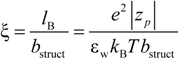
26]. According to the Manning model, the system is characterized by a charge-density parameter ξ, defined as the ratio of the Bjerrum length
lB and the structural charge spacing
bstruct :
where ε
w is the permittivity of the aqueous phase and
KBT the thermal energy. Here, the Bjerrum length is defined as the length scale at which the Coulomb interaction between two elementary charges in a dielectric medium with a dielectric constant ε
w is equal to the thermal energy
KBT.
If the charge spacing is too small, the electric field becomes so strong that the system can lower its free energy by condensing some of the counterions on the polyion chain. If:
Counterions of valence
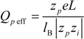
z1 become trapped close to the polyion chain (counterion condensation) to reduce its effective charge from the value
Qp =
zpeN (before condensation) to the effective value:
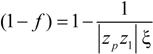
So that the fraction of free (un-condensed) counterions will be:
and the fraction of condensed counterions, and consequently, the fraction of charges on the polyion chain, will result:
The charged polyion, together with the condensed counterions, can be considered as a single entity with an effective charge Qp eff which is considerably lower than the bare structural charge Qp.
Within this model, polyion and condensed counterions, under the influence of an external electric field, move together with the same mobility
up. However, in the infinite polyion length limit and in the presence of high salt content, simulations have recently shown that this motion decouples and condensed counterions acquire a mobility with respect to the polyion itself [
27].
It must be noted that condition (1.4) strictly holds in the case of an infinite isolated linear polyion chain. In the case of finite length rod-like polyions, at a finite concentration, a counterion condensation theory has been, more recently, developed by Netz [
28] and Manning and Mohanty [
29] who derived a more general condition, depending on the length of the polyion chain. However, in practice, in most cases, polyions are long enough to be in the regime described by Equation (1.4) and only short oligomers, exhibiting an incomplete condensation, deviate from this behavior.
From a physical point of view, counterion condensation is due to a balance between a favorable gain in electrostatic energy as a consequence of the ion collapse and an unfavorable loss of entropy when counterions bind to the polymer chain. This phenomenon plays an important role in biological polyelectrolyte solutions since the effective charge on the polyion backbone affects the morphology of the polyelectrolyte itself and, moreover, its response to external stimuli.
A typical example of counterion condensation occurs in DNA chains, where data obtained from optical tweezers experiments [
30] indicate that the effective charge is −050 ± 0.05 per base pair, much less than the bare charge −2 per base pair (two phosphates per base pair), equivalent to a reduction of the bare charge by 75% ± 3%, in excellent agreement with the reduction predicted by the Manning counterion condensation theory of 76%.
During the last decades, a number of studies have focused on the phenomenon of counterion condensation, both experimental [
31,
32] and theoretical, and by simulations [
33,
34].
2. The Electrical Conductivity. Theoretical Background and Basic Equations
In order to put things into their proper perspective, we will start by describing the theory of the electrical conductivity of an aqueous solution.
From a phenomenological point of view, the electrical conductivity of an aqueous solution of polyelectrolytes originated by the movement of any charged entity in response to an external applied electric field, depends on three independent contributions,
i.e., the numerical concentration
ni of the charge carriers of type
i, their electrical charge (
zie) and their mobility
ui, according to the relationship:
Here, the mobility
u is defined as the ratio of the average velocity of the charged carrier to an applied electric field of unit strength. From an experimental point of view, the usual definition of the conductivity
σ is given by the linear relationship:
between the volume averaged current density
![Polymers 06 01207 i008]()
:
and the measured electric field
![Polymers 06 01207 i010]()
:
where φ(
![Polymers 06 01207 i012]()
) is the electrical potential at position
![Polymers 06 01207 i012]()
and
V is a sufficient large volume of the system.
Equation (2.1) can be written in a more usual way if we express the numeric concentration
ni through the molar concentration
Ci (
ni =
NACi, where
NA is the Avogadro number) and the mobility
ui through the equivalent conductance λ
i (
ui = λ
i /
F, where
F =
eNA is the Faraday constant). We obtain:
In cgs units, the concentrations Ci are expressed in [mol/cm3] and the equivalent conductances in [statohm−1·cm2·mol−1] (for the conversion to SI units, 1 statohm ≈ 9 × 10¹¹ ohm). Equation (2.5) is the basic equation that governs the whole transport process, depending on the concentration Ci and the equivalent conductance λi of each charge carrier.
In the case of a polyelectrolyte solution, charge carriers derive from the partial dissociation of the polyion chain and Equation (2.5) can be rewritten as:
where the subscripts “1” and “p” refer to counterions and polyions, respectively.
Because of the counterion condensation effect, the following relationships hold,
i.e.,
C1 =
v1N f Cp,
Z1 =
z1,
Zp =
N f zp, and Equation (2.5) reduces to:
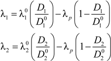
The equivalent conductance λ
1 differs from the value
![Polymers 06 01207 i014]()
of the counterion in the absence of the polyelectrolyte, according to:
where
![Polymers 06 01207 i016]()
and
![Polymers 06 01207 i077]()
are the diffusion coefficients of counterions in the limit of infinite dilution and in the presence of polyions, respectively.
With this substitution, Equation (2.7) becomes:
taking advantage of the fact that |
zp| −
v1|
z1| = 0. In the light of this framework, the parameters which define the electrical conductivity of the polyelectrolyte solution are the equivalent conductance λ
p of the polyion chain, the fraction
f of free (un-condensed) counterions, besides the degree of polymerization
N and the polyion concentration
Cp.
The Equivalent Conductance in the Manning Model
Before going on, we summarize the main results of the Manning model [
24,
25,
26] as far as the equivalent conductance λ
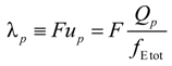
p is concerned. In this context, the equivalent conductance λ
p can be written as the ratio of the polyion charge
Qp and the total electrophoretic coefficient
fEtot according to the expression:
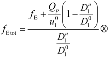
where
F is the Faraday constant and the total electrophoretic coefficient, corrected for the
asymmetry field effect, can be writes as:
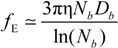
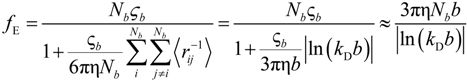
If the electrophoretic coefficient
fE is calculated according to the general expression given by Kirkwood and Riseman [
32], modeling the polyion as an ensemble of
Nb simple spherical units of radius
Rb, following the Manning derivation, we have:
where ς
b = 6πη
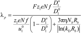
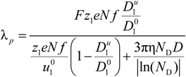
Rb is the friction coefficient, with η the viscosity of the aqueous phase. The final expression for the equivalent conductance λ
p of the polyion can be written as:
where
![Polymers 06 01207 i023]()
is the inverse of the Debye screening length and
![Polymers 06 01207 i024]()
is the mobility of counterions in the limit of infinite dilution.
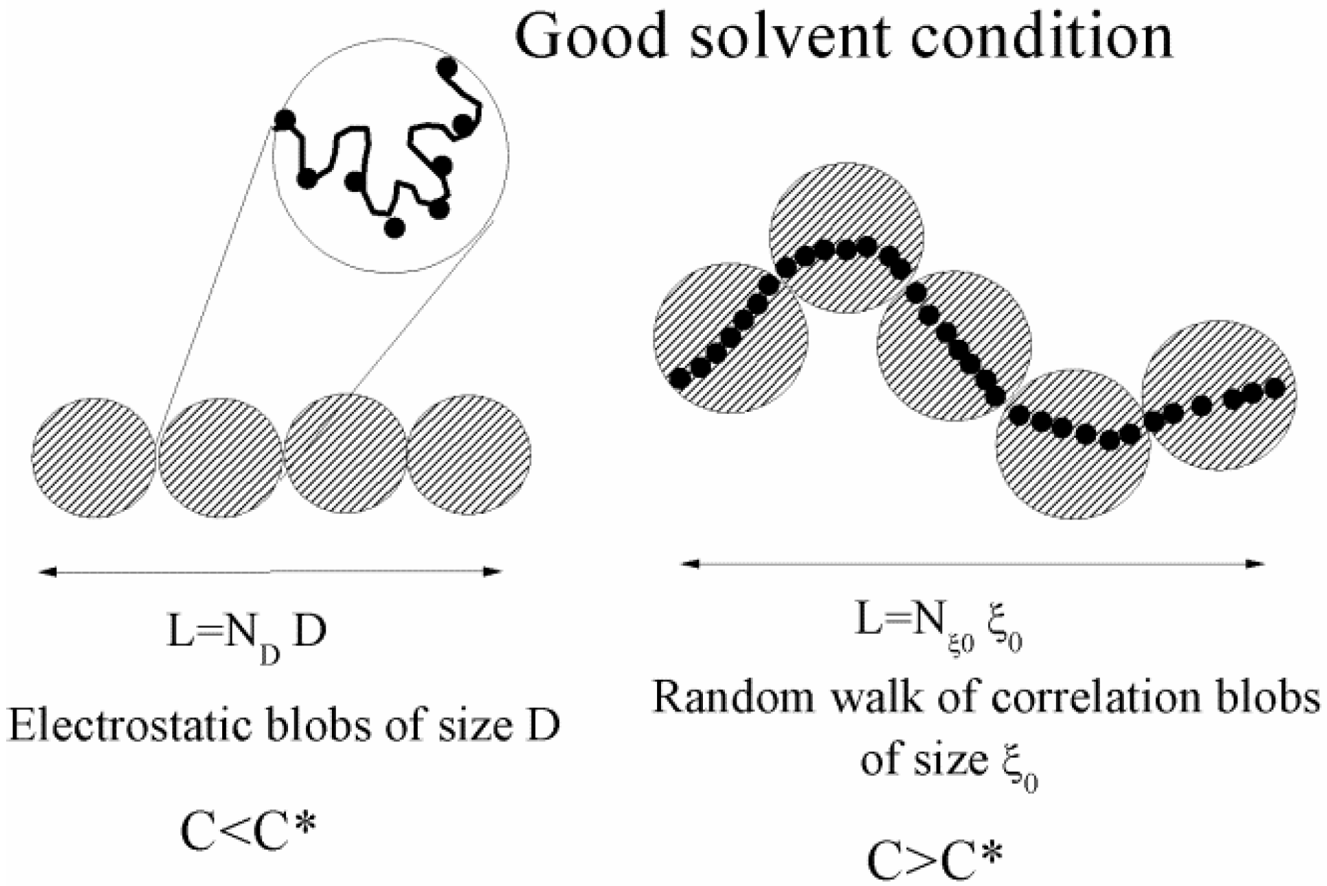
Figure 1.
A sketch of a polyelectrolyte chain in good-solvent conditions, for different (salt free) concentration regimes. The chain is an extended rodlike configuration of electrostatic blobs and a random walk of correlation blobs for dilute (C < C*) and semidilute (C > C*) regimes, respectively.
Figure 1.
A sketch of a polyelectrolyte chain in good-solvent conditions, for different (salt free) concentration regimes. The chain is an extended rodlike configuration of electrostatic blobs and a random walk of correlation blobs for dilute (C < C*) and semidilute (C > C*) regimes, respectively.
The second example is taken from reference [
12]. We have investigated the electrical behavior of poly(N-methyl-2-vinyl pyridinium chloride) [PMVP-Cl] at two different charge densities in two different solvents,
i.e., pure water (poor-solvent condition) and ethylene glycol (good-solvent condition). These polymers possess a carbon-based backbone for which water is a poor solvent and ethylene glycol behaves as a good solvent.
4. Poor Solvent Condition
Polymer-solvent interactions are of primary importance in determining the spatial configuration of the polymer chain in solution. In the light of the scaling approach, the configuration of a hydrophobic chain in a poor solvent condition has been discussed extensively by Dobrynin and Rubinstein [
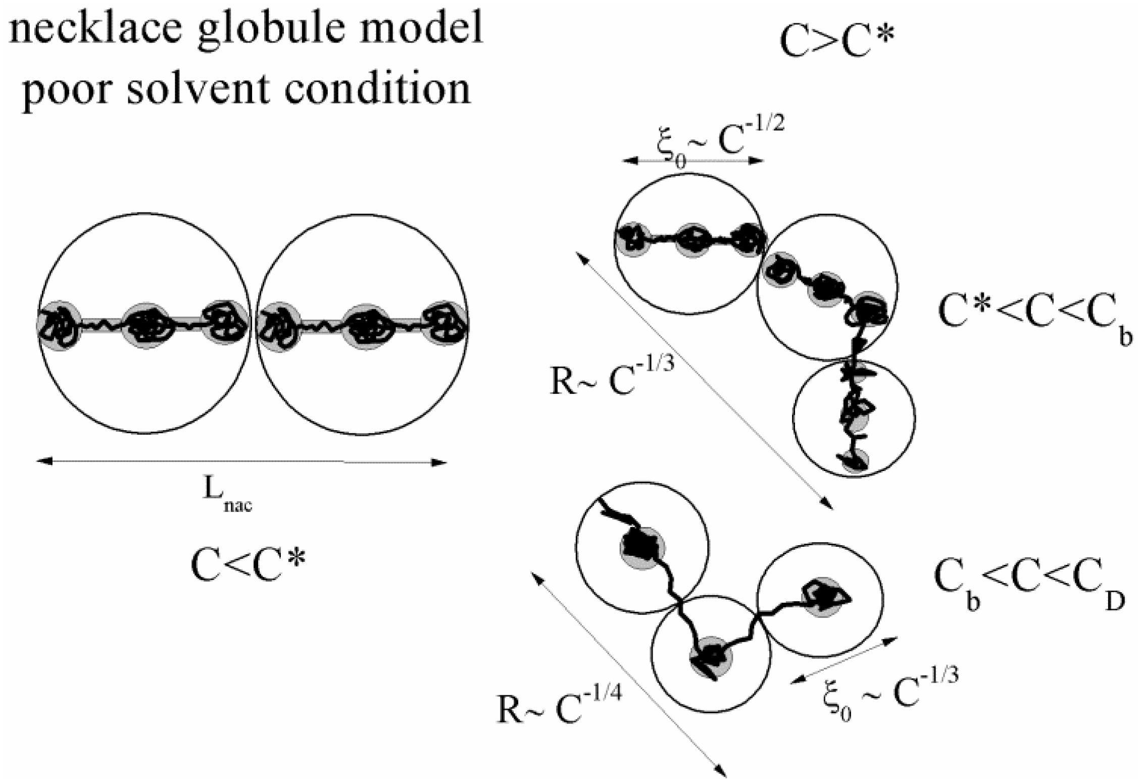
36], who developed a scaling theory of hydrophobic polyelectrolytes over the entire range of polyelectrolyte concentrations and postulated the so-called necklace globule model.
Due to the strong hydrophobic interactions between the polymer backbone and the water molecules, in poor solvent conditions, the electrostatic blobs or the correlation blobs, present when good solvent condition applies, will split into a set of smaller charged globules (beads) connected by long and narrow tubules (strings). As pointed out by Dobrynin [
36], this structure optimizes the correlation-induced attraction of condensed counterions to charged monomers and electrostatic repulsion between ionized charges.
The situation is even more interesting in the case of semidilute regime (C > C*), where two new different concentration regimes appear, i.e., string controlled regime (C* < C < Cb) and bead controlled regime (Cb < C < CD), where a different concentration dependence of the chain size occurs.
In string-controlled regime, the correlation length is much larger than the size of the beads and the chains assume a bead-necklace structure on length scales smaller than the correlation length. Conversely, in bead-controlled regime, the correlation length is of the order of the size of the beads and the chains assume a bead structure on length scales smaller than the correlation length [
37]. This effect is analogous to the splitting of a charged liquid droplet into an array of smaller ones, as predicted by Rayleigh long ago [
38]. These different regimes imply a different picture of counterion condensation, which will condense on the necklace globule in an avalanche-like fashion. As pointed out by Jeon and Dobrynin [
39], with the increase of the polyion concentration, counterions condense inside beads of the necklace globule, favoring the reduction of its charge and the increase of its mass which further promote the counterion condensation giving rise to the avalanche-like process. The necklace conformation is supported by experiments [
40] and computer simulations [
41,
42].
A sketch of the necklace globule model is shown in
Figure 2.
Figure 2.
A sketch of the necklace globule model for a polyion in poor solvent condition, in dilute (C < C*) and semidilute (C > C*) concentrations. The semidilute concentration splits into string controlled regime (C* < C < Cb) and bead controlled regime (Cb < C < CD).
Figure 2.
A sketch of the necklace globule model for a polyion in poor solvent condition, in dilute (C < C*) and semidilute (C > C*) concentrations. The semidilute concentration splits into string controlled regime (C* < C < Cb) and bead controlled regime (Cb < C < CD).
4.1. Dilute Solutions
When the total effective charge of a polyion Qp = zefN becomes larger than Q'= ze(Nτb / lb)1/2 and the Coulomb repulsion becomes comparable to the surface energy, the system tends to reduce its total free energy giving rise to Nb beads of size Db containing monomers each and joined (Nb − 1) strings of length ls. The length of the necklace is given by Lnec = Nbls, since the most of the length is stored in the string (ls >> Db).
The quality of the solvent is taken into account by the solvent quality parameter τ defined as τ =
![Polymers 06 01207 i030]()
, where θ is the temperature at which the net excluded volume for uncharged monomers is zero.
In this case, the friction coefficient
fE can be written as:
The characteristic quantities scale as:
4.2. Semidilute Solutions
The overlapping concentration
Cb between the string controlled regime (
C* <
C <
Cb) and the bead-controlled regime (
Cb <
C <
CD) depends, in addition to the monomer size
b and the fraction
f, on the solvent quality parameter τ and scales according to the relationship:
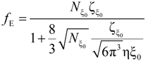
In the string-controlled regime C* < C < Cb, the chain is assumed to be a random walk of Nξ0 = N / gξ correlation segments of size ξ0, each of them containing gξ monomers.
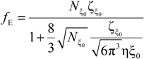
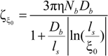
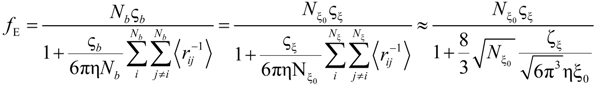
The electrophoretic friction coefficient is given by:
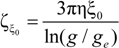
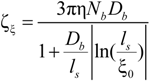
where the friction coefficient ζ
ξ is given by:
The characteristic quantities scale as:
In the bead-controlled regime Cb* < C < CD, owing to the screening of the electrostatic interactions between beads, the model predicts only one bead per correlation globule of size ξ0, containing gξ monomers.
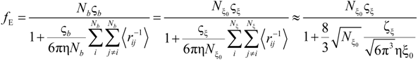
The electrophoretic friction coefficient is given by:
where the friction coefficient ζ
ξ is given by:
The characteristic quantities scale as:
4.3. The Diffusion Coefficients ![Polymers 06 01207 i016]() and
and ![Polymers 06 01207 i077]() in the Light of the Scaling Approach
in the Light of the Scaling Approach
To proceed further to the calculation of the polyion equivalent conductance λ
p and, finally, to the electrical conductivity σ of the polyelectrolyte solution, the ratio
![Polymers 06 01207 i016]()
/
![Polymers 06 01207 i077]()
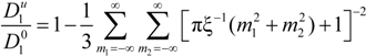
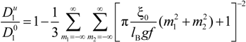
must be appropriately evaluated in the light of the scaling laws. In the presence of counterion condensation (but in the absence of added salt), Manning [
25] derived the following expression:
with (
m1,
m2) ≠ (0,0) and ξ = 1/|
z1zp|. In the case of uni-univalent polyion (
z1 =
zp = 1), for ξ = 1, numerical evaluation of Equation (4.3.1) yields a constant value
![Polymers 06 01207 i016]()
/
![Polymers 06 01207 i077]()
≃ 0.866.
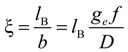
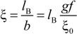
Within the scaling picture, the charge density parameter ξ can be written as:
in electrostatic blob model (dilute concentration) and:
in correlation blob model (semidilute concentration).
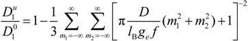
Consequently, the ratio
![Polymers 06 01207 i016]()
/
![Polymers 06 01207 i077]()
assumes the expression:
for dilute regime and:
for semidilute regime.
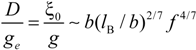
In the light of the scaling laws, the two relevant quantities
D /
ge and ξ
0 /
g scale, in good solvent condition, as:
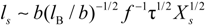
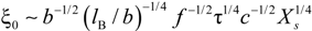
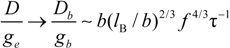
In poor solvent condition, in dilute regime the following substitution hold:
whereas, in semidilute regime we have:
which scale as:
in string controlled regime and in bead controlled regime, respectively.
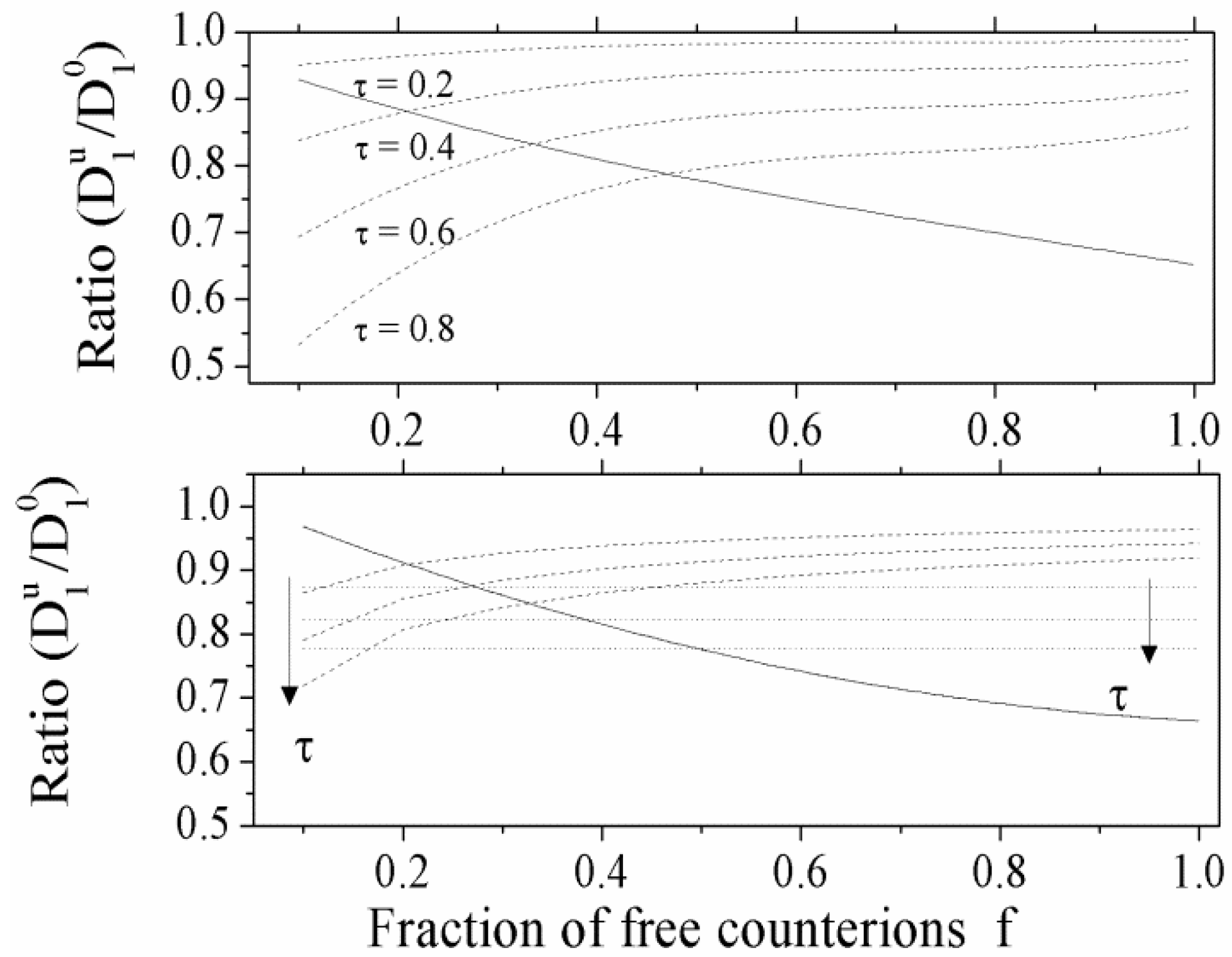
Typical behavior of the ratio
![Polymers 06 01207 i016]()
/
![Polymers 06 01207 i077]()
as a function
f of the fraction of the free counterions, in dilute and semidilute regimes, is shown in
Figure 3.
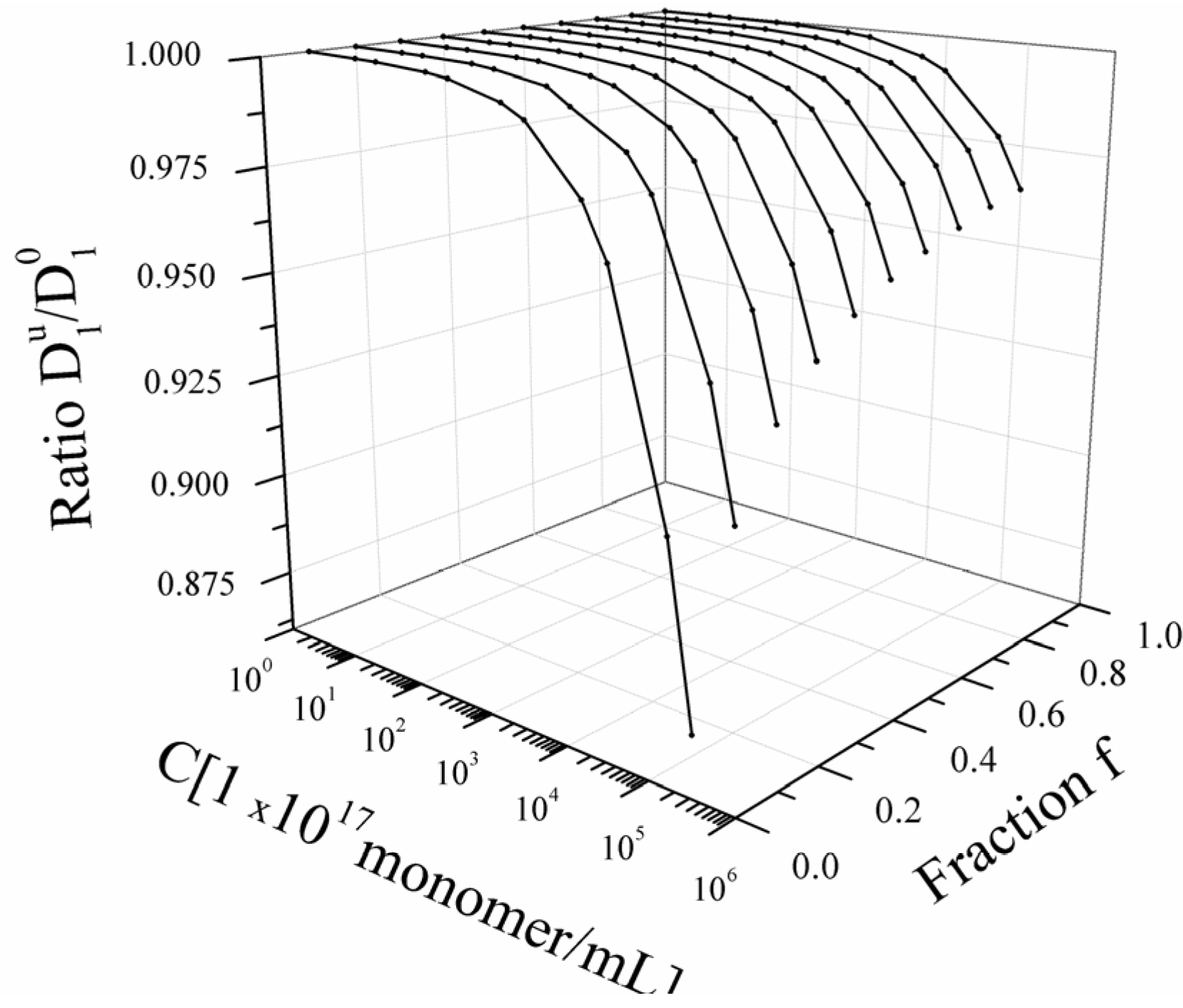
As can be seen in Equation (4.3.9), in bead controlled regime, there is, contrarily to the other regimes, a dependence on the polyelectrolyte concentration
c (expressed as monomers per unit volume). In
Figure 4, the typical dependence of
![Polymers 06 01207 i016]()
/
![Polymers 06 01207 i077]()
on the concentration
c, for different values of the fraction
f is shown in
Figure 4. In this case, the value of the parameter
τ is assumed fixed to τ = 0.4.
Figure 3.
(Upper panel): the ratio
![Polymers 06 01207 i016]()
/
![Polymers 06 01207 i077]()
for polyelectrolytes solution in dilute regime; full line: good solvent condition; dotted lines: poor solvent condition, with four different values of the parameter τ (τ = 0.2, 0.4, 0.6, 0.8). (Bottom panel): the ratio
![Polymers 06 01207 i016]()
/
![Polymers 06 01207 i077]()
for polyelectrolytes solution in semidilute regime. Full line: good solvent condition. Dotted lines: poor solvent condition, in string-controlled regime. Dashed lines: poor solvent condition, in bead-controlled regime with different values of the parameter τ (τ = 0.4, 0.6, 0.8, in the order marked by the arrow).
Figure 4.
Bead-controlled regime. Dependence of the ratio
![Polymers 06 01207 i016]()
/
![Polymers 06 01207 i077]()
on the polyelectrolyte concentration
C and on the fraction
f for a fixed value of the solvent quality parameter (τ = 0.4).
Figure 4.
Bead-controlled regime. Dependence of the ratio
![Polymers 06 01207 i016]()
/
![Polymers 06 01207 i077]()
on the polyelectrolyte concentration
C and on the fraction
f for a fixed value of the solvent quality parameter (τ = 0.4).
From the above analysis, it turns out that the electrical conductivity of a polyelectrolyte solution in the absence of added salt depends essentially on two parameters, the fraction f of free counterions and the solvent quality parameter τ. These parameters control the polyion equivalent conductance λp in the different concentration regimes (dilute and semidilute concentrations), according to the above stated scaling relationships.
A typical dependence of the equivalent conductance λ
p of the polyion in poor-solvent condition as a function of the polymer concentration, covering both the dilute and semidilute regime, is shown in
Figure 5. As can be seen, the dependence is rather complex, reflecting the different conformations assumed by the polyion chain in the different concentration regimes.
Figure 5.
Behavior of the equivalent conductance λp of polyions in poor-solvent condition, as a function of the polyion concentration. According to the scaling picture, three different concentration regimes are clearly shown. In the dilute regime, the conductance is independent of the concentration. In the semidilute regime, a string-controlled regime and a beads-controlled regime are dependent on the concentration.
5. Polyelectrolyte Solutions in the Presence of Added Salt
Following an additive rule, in the presence of added salt, Equation (2.7) must be replaced by:
where, in analogy with the symbols adopted for the polyion contribution, the last two terms represent the contribution given by ions due to the dissociation of the salt molecules.
In this case too, the equivalent conductances λ can be writes as:
Substitution of Equation (5.2) into Equation (5.1) yields:
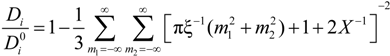
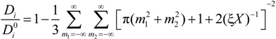
The general expression for the ratio (
Di /
![Polymers 06 01207 i017]()
) (
i = 1,2), according to the derivation proposed by Manning [
24,
25], can be written as:
in the case of absence of counterion condensation and as:
in the case of counterion condensation.
Here, ξ is, as usual, the charge density parameter and X, that takes into account the ratio of salt and polyion concentration, is defined as X = NCp / Cs.
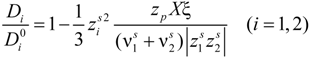
To a first approximation, Equations (5.4) and (5.5) can be simplified according to the following expression:
and Equation (5.3) assumes two different expressions whether or not there is counterion condensation. In the first case, in absence of counterion condensation,
i.e., ξ < 1 / |
zpz1|, Equation (5.3) becomes:
Equation (5.7) reduces to the usual expression in the case of uni-univalent salt and for univalent charges on the polyion chain. In this case,
zp = 1;
z1 = 1;
v1 =1;
![Polymers 06 01207 i052]()
=1;
![Polymers 06 01207 i053]()
= 1;
![Polymers 06 01207 i054]()
= 1;
![Polymers 06 01207 i054]()
= 1 and the expression for the conducibility becomes:
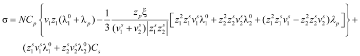
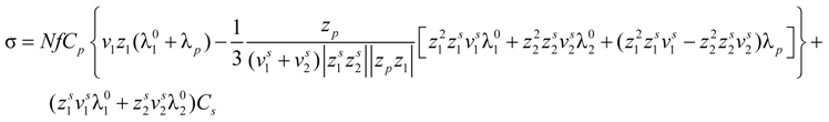
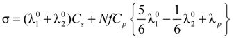
In the presence of counterion condensation,
i.e., ξ > 1/|
zpz1|, Equation (5.3) can be written as:
that, analogously to the previous case, for univalent charges, reduces to:
As can be seen, in Equations (5.5) and (5.7), or equivalently, in the Equations (5.6) and (5.8), the key parameter that governs the conductometric behavior of the polyion solution is represented by the polyion equivalent conductance λp which contains all the relevant information concerning the concentration regimes and the polyion conformation.
As previously done, we will start considering the equivalent conductance λp within the Manning model and how, in the framework of the scaling relationships, this parameter has to be modified as a function of the polyion concentration, the quality of the solvent.
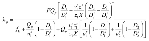
Taking into account the “asymmetry field” correction, in the presence of added salt, the general expression for the polyion equivalent conductance λ
p given by Manning, reads:
where
fE is the electrophoretic coefficient (without the asymmetry field correction),
X =
Nnp /
ns ≡
c /
ns takes into account the ratio of the salt and polyion concentration and
![Polymers 06 01207 i060]()
and
![Polymers 06 01207 i061]()
are the cation and anion mobilities in the aqueous phase (in the absence of the polyion). Here, the polyion charge
Qp depends on the charge density parameter and stands for
Qp =
zpeNf in the presence of counterion condensation and for
Qp =
zpeN (the structural value) in the absence of counterion condensation.
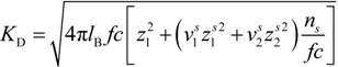
The electrophoretic coefficient
fE in the light of the Manning model is approximated by:
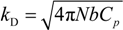
where the inverse of the Debye screening length is given by:
5.1. The Scaling Approach
In the presence of added salt, the polyion conformation is characterized by three different concentrations that define different concentration regimes. These concentrations are the concentration C* at which the distance between chains equals their extended length, the concentration CD where the electrostatic blobs begins to overlap, and the concentration Ce (in between C* and CD) at which polymer chains begin to entangle. Consequently, the polymer solution behaves as dilute solution for C < C*, as un-entangled semidilute solution for C* < C < Ce and as entangled semidilute solution for Ce < C < CD. Finally, polymer solution behaves as concentrated solution for C > CD.
In analogy with what we have done in the previous section, we will discuss good-solvent and poor-solvent conditions, separately.
5.1.1. Good-Solvent Condition
In the dilute concentration regime, the polyion chain is represented by a self-avoiding walk of NrB electrostatic blobs of size rB inside which the polyion conformation is extended. Each electrostatic blob contains gB monomers and bears an electric charge qrB = zpefgB. The polyion bears a charge Qp = NrBqrB, assuming a flexible conformation with an end-to-end distance given by R = rB(N / gB)3/5.
In the semidilute concentration regime, the polyion chain is modeled as a random walk of
Nξ0 =
N /
g correlation blobs of size ξ
0. Each correlation blob bears an electric charge
![Polymers 06 01207 i078]()
=
zpefg while the polyion charge is
Qp =
![Polymers 06 01207 i078]() Nξ0
Nξ0. In this case, the polyion end-to-end length is given by
R = ξ
0(
N /
g)
1/2.
Contrarily to what happens in the absence of added salt, in this case, electrostatic interactions are reduced by the presence of the added salt and in both the two regimes a random-walk structure dominates.
5.1.2. Poor-Solvent Condition
In dilute concentration regime, when the effective polyion charge becomes larger than a critical value and the Coulombic repulsion becomes comparably with the surface energy, the polyion splits into
Nb beads of size
Db and joined by (
Nb − 1) strings of length
ls. In the semidilute concentration regime, the concentration
Cb introduces, in analogy with the case in absence of added salt, two different regimes. In string-controlled regime (
C* <
C <
Cb), the chain is composed of
Nξ0 =
N /
![Polymers 06 01207 i079]()
correlation segment of size ξ
0 each of them containing
![Polymers 06 01207 i079]()
monomers. The chain is assumed to be a random walk of size
R = ξ
0(
N /
![Polymers 06 01207 i079]()
)
1/2. In the bead-controlled regime (
Cb <
C <
CD), the screening of the electrostatic interactions produces one bead per correlation globule with a random walk chain conformation of size
R = ξ
0(
N /
![Polymers 06 01207 i079]()
)
1/2, analogous to the size of the chain in string-controlled regime.
5.2. The Electrophoretic Coefficient fE
As in the previous cases, in the presence of added salt too, the electrophoretic coefficient fE depends on the different concentration regimes, since the elementary unit that contributes to the conductivity, in the light of the Manning theory, differs from a regime to the other.
In good solvent condition and in dilute regime, the elementary unit is the electrostatic blob of size
Db and the electrophoretic coefficient
fE is given by:
In good-solvent condition, but in semidilute regime, the elementary unit is the correlation blob of size ξ
0 and the electrophoretic coefficient
fE is given by:
with the friction coefficient ζ
ξ0 given by:
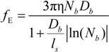
In the poor solvent condition, when the necklace model applies, the electrophoretic coefficient
fE in the dilute regime (the elementary unit is the bead of size
Db) is given by:
and in the semidilute regime (the elementary unit is the blob of size ξ
0) is given by:
In this latter case, the friction coefficient ζ
ξ0, depending on the basic unit of the chain, can be written as:
in the semidilute string controlled regime (
C* <
C <
Cb) and as:
in the semidilute bead-controlled regime (
Cb <
C <
CD).
In good solvent condition, according to the scaling theory, the characteristic quantities are
Db and
Nb in dilute regime and ξ
0,
Nξ0 and
g /
ge in semidilute regime. These quantities scale as:
for the dilute regime and as:
for the semidilute regime.
In poor solvent condition, according to the scaling relationships, the characteristic quantities entering Equations (5.2.4) and (5.2.5) are
Nb,
Db and
ls in the dilute regime and ξ
0,
Nξ0 in the semidilute regime. These quantities scale as:
in the dilute regime and as:
in the semidilute string-controlled regime and, finally, as:
in the semidilute bead-controlled regime.
Here, the quantity
Xs, that takes into account the concentration of free ions present in the solution, is defined as:
For uni-univalent salt and for univalent counterions, the equation reduces to:
On the basis of these scaling relationships, the equivalent conductance λ
p can be conveniently evaluated in each concentration regime we are dealing with, taking into account the appropriate quality of the solvent. Once the equivalent conductance λ
p is known, the electrical conductivity σ of the whole polyelectrolyte solution derives directly from the Manning expression. As an example, in
Figure 6 we report the equivalent conductance λ
p for polyions in good-solvent condition, in dilute and semidilute regime and in the presence of added salt.
Figure 6.
The equivalent conductance λ
p of polyions in good solvent regime, for dilute and semidilute conditions, calculated according to Equations (5.2.1) and (5.2.2) in the presence of added salt, for three different values of the parameter
X. Dotted lines show the calculated values in the dilute region extrapolated to semidilute region. The parameters are:
N = 2250;
lB = 7 × 10
−8 cm;
b = 2.52 × 10
−8 cm; η = 1 cP;
![Polymers 06 01207 i060]()
= 0.137 cgs units;
![Polymers 06 01207 i061]()
= 0.235 cgs units. Here,
X is defined as
X =
c/
ns.
6. Comparison with Experiments
In what follows, we will compare some representative results from the recent literature with the ones predicted by the scaling theory. We confine ourselves to one’s own measurements [
4,
5,
8,
12], but in the recent literature many other appropriate examples can be easily found.
Electrical conductivity measurements of Sodium polyacrylate salts [−CH
2CH(CO
2Na)−]
n, [NaPAA] as a function of polymer concentration to cover the dilute and semidilute regime have been extensively reported in Reference [
5]. Measurements have been carried out at three different values of the ratio
X =
c /
ns (
X = 0.1, 1, 10), by adding appropriate amount of NaCl electrolyte solution, maintaining constant the ratio between the number of monomers and the number of ions derived from the added salt. In these experiments, good-solvent condition applies. In
Figure 7, we show a comparison between the polyion equivalent conductance λ
p directly derived from the experimental values of the electrical conductivity σ and the values calculated on the basis of the scaling approach we have above discussed. As can be seen, both in the dilute regime and in the semidulute regime, the agreement is quite good. In particular, we observe that transition from dilute and semidilute regime occurs exactly at the polyion concentrations predicted by the theory.
Figure 7.
The equivalent conductance of NaPAA polyions in aqueous solutions in the presence of added salt (
X = 0.1, = 1,
X = 10) as a function of the polyion concentration. Polymer in good solvent condition. Panel (
A) Dilute solution,
X = 0.1; (■) experimental values derived from the measured electrical conductivity. Full curve is calculated on the basis of Equation (5.2.1). Panel (
B) Dilute and semidilute solution, the transition region being marked by the arrow,
X = 1; (●) experimental values derived from the measured electrical conductivity. Upper full curve is calculated on the basis of Equation (5.2.1) in the dilute regime and lower full curve calculated on the basis of Equation (5.2.2) in the semidilute regime. Panel (
C) Dilute and semidilute solution, the transition region being marked by the arrow.
X = 10; (●) experimental values derived from the measured electrical conductivity. Upper full curve is calculated on the basis of Equation (5.2.1) in the dilute regime and lower full curve calculated on the basis of Equation (5.2.2) in the semidilute regime. Data redrawn from Reference [
5].
![Polymers 06 01207 g007]()
The second example is taken from reference [
12]. We have investigated the electrical behavior of poly(N-methyl-2-vinyl pyridinium chloride) [PMVP-Cl] at two different charge densities in two different solvents,
i.e., pure water (poor-solvent condition) and ethylene glycol (good-solvent condition). These polymers possess a carbon-based backbone for which water is a poor solvent and ethylene glycol behaves as a good solvent.
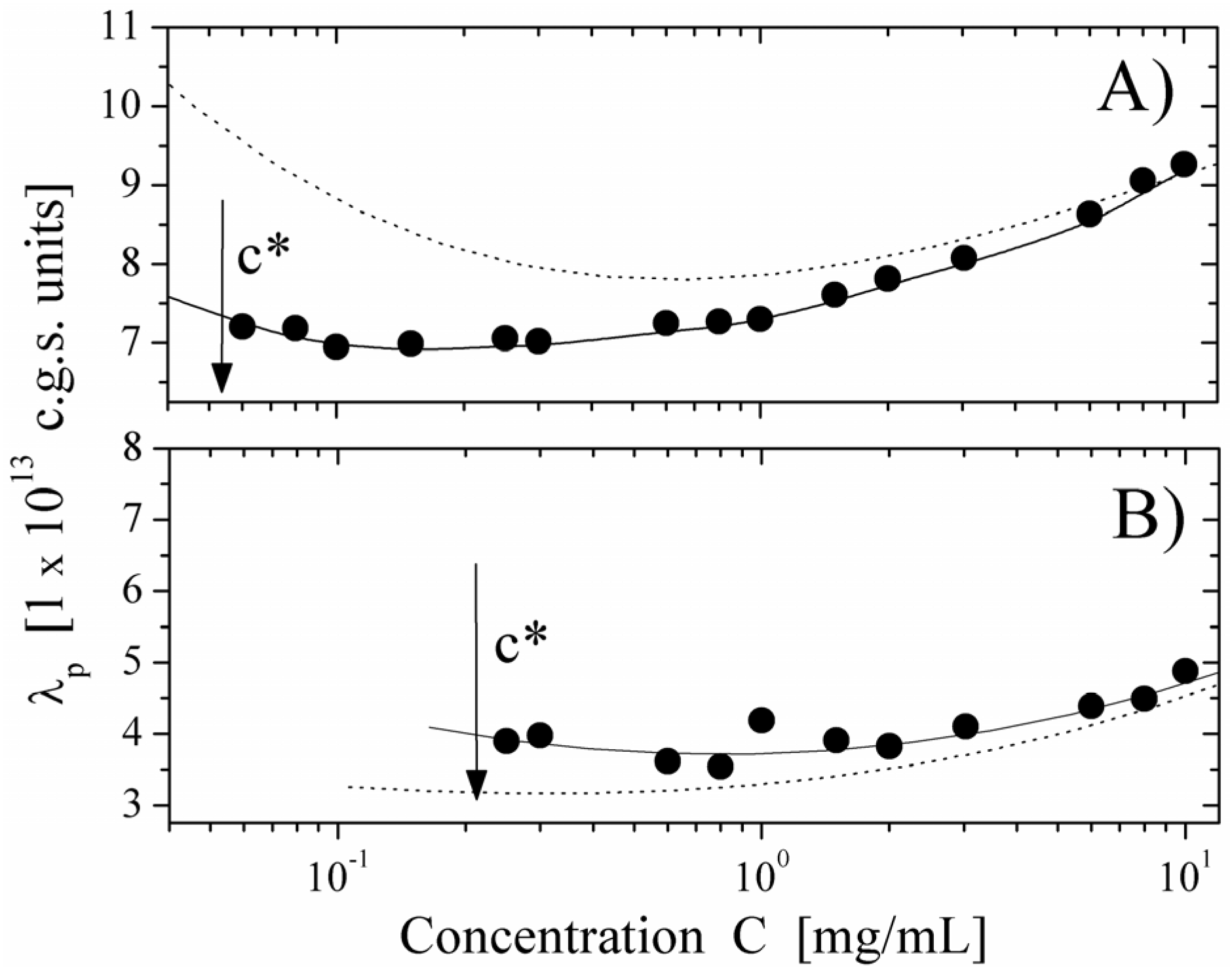
We report here some typical results showing the behavior of the equivalent conductance λ
p of the polyion as a function of the polyion concentration, derived from the measured electrical conductivity and compared with the values calculated, on the basis of the scaling approach, for semidilute regime in string-controlled conditions. We present two limiting cases,
i.e., polyions in water (poor-solvent condition) and in ethylene glycol (good-solvent condition) in cases of differently charged poyions (
Figure 8, degree of quaternization
Q = 55% and
Figure 9, degree of quaternization
Q = 17%). As can be seen, the agreement with the expected behavior is quite good over the whole concentration range, where the semidilute regime holds. This agreement is further enforced if we compare the values of the equivalent conductance for water solution with the ones calculated for good solvent condition (dotted line in
Figure 8 Panel A) or for ethylene glycol with the ones for poor-solvent conditions (dotted line in
Figure 8. Panel B).
These results are a strong support for the necklace model for hydrophobic polyions in the light of the dynamic scaling models.
Figure 8.
The equivalent conductance of 55% PMVP-Cl (
Q = 55%) polyion as a function of concentration
C. Panel (
A) polyion in water solution (poor-solvent condition). (●): values derived from the measured electrical conductivity. Full line represents the corresponding values calculated according to the necklace model in the semidilute string-controlled condition, assuming = 0.6. The dotted line represents the calculated values in the semidilute good-solvent condition. Panel (
B) polyion in ethylene glycol solvent (good-solvent condition). (●): values derived from the measured electrical conductivity. Full line represents the corresponding values calculated according to the semidilute good-solvent condition. The dotted line represents the calculated values in the necklace model in semidilute-string-controlled condition. The arrow marks the concentration
c *, indicating the transition between the dilute and the semidilute regime. Data from Reference [
12].
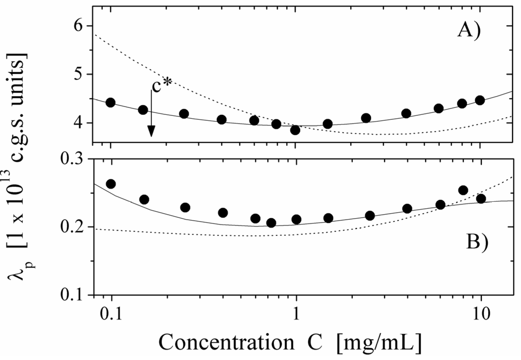
Figure 9.
The equivalent conductance of 17% PMVP-Cl (
Q = 17%) polyion as a function of concentration
C. Panel (
A) polyion in water solution (poor-solvent condition). (●): values derived from the measured electrical conductivity. Full line represents the corresponding values calculated according to the necklace model in the semidilute string-controlled condition, assuming τ = 0.6. The dotted line represents the calculated values in the semidilute good-solvent condition. Panel (
B) polyion in ethylene glycol solvent (good-solvent condition). (●): values derived from the measured electrical conductivity. Full line represents the corresponding values calculated according to the semidilute good-solvent condition. The dotted line represents the calculated values in the necklace model in semidilute-string-controlled condition. The arrow marks the concentration
c *, indicating the transition between the dilute and the semidilute regime. Data from Reference [
12].


 :
:
 :
:
 ) is the electrical potential at position
 of the counterion in the absence of the polyelectrolyte, according to:
 and
and  are the diffusion coefficients of counterions in the limit of infinite dilution and in the presence of polyions, respectively.
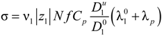
 is the inverse of the Debye screening length and
  is the mobility of counterions in the limit of infinite dilution.
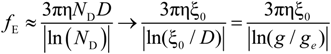
 is much larger than the average distance between chains and charges are obliged to interact by means of an unscreened Coulombic potential. In these conditions, the polymer chain is represented by an extended rod-like configuration of ND electrostatic blobs of size D to form a fully extended chain of length L = NDD. Each electrostatic blob contains ge monomers and bears a charge qD = zpe f ge. As usual, f is the fraction of ionized charged groups on the polymer chain and consequently the fraction of free counterions. The total charge of each polyion chain is Qp = qDND ≡ zpe f geND.
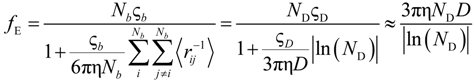
 = zpefg and the charge of the full chain is Qp =
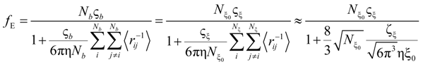
 , where θ is the temperature at which the net excluded volume for uncharged monomers is zero.
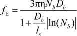


 ) (i = 1,2), according to the derivation proposed by Manning [24,25], can be written as:
 =1;
=1;  = 1;
= 1;  = 1;
= 1; 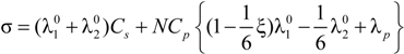
 and
and  are the cation and anion mobilities in the aqueous phase (in the absence of the polyion). Here, the polyion charge Qp depends on the charge density parameter and stands for Qp = zpeNf in the presence of counterion condensation and for Qp = zpeN (the structural value) in the absence of counterion condensation.
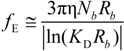
 correlation segment of size ξ0 each of them containing