In this section, first the batch bulk ICAR ATRP of MMA and
nBuA for the synthesis of “MMA-
nBuA gradient copolymers” is studied as a function of the initial Cu(II) ppm level at a polymerization temperature of 80 °C, considering the reference system defined in
Table 1. Next, it is shown that fed-batch procedures are beneficial compared to batch ICAR ATRP under similar overall conditions (e.g., same overall amount of conventional radical initiator). Both single- and multi-component fed batch additions are considered and the relevance of the nature of the conventional radical initiator is highlighted.
3.1. Batch Procedure
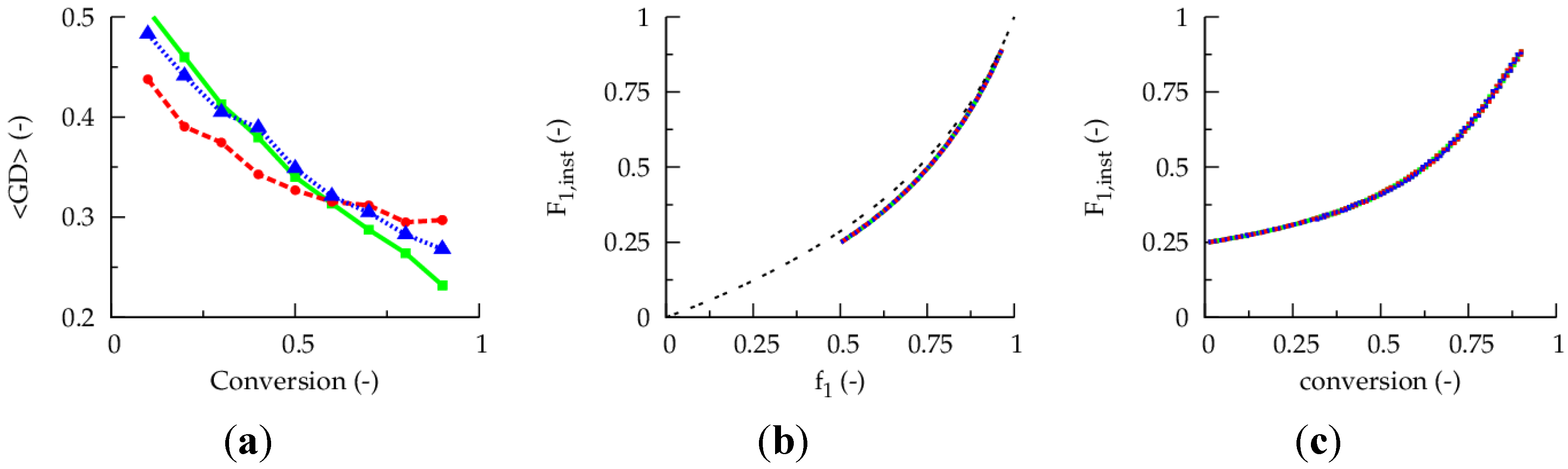
Figure 1a presents the evolution of the gradient deviation (<GD>) as a function of conversion for a polymerization temperature of 80 °C, a TCL of 100 and an initial Cu(II) ppm level of 10, 30 and 50 ppm (dashed red, dotted blue and full green line). The selected conventional radical initiator is AIBN and equimolar initial comonomer amounts are applied. Note that such equimolar amounts are selected as conversions leading to almost complete monomer depletion are envisaged for illustration purposes. For a reliable <GD> calculation, the monomer sequences of
ca. 150,000 copolymer chains are tracked explicitly. It can be seen that the selected ppm level influences the linear gradient quality. Only for the highest ppm level of 50, a <GD> value below 0.25 can be reached at high conversion, implying the necessity of a minimum amount of ATRP catalyst in the reaction medium under batch conditions.
However, as shown in
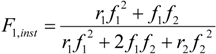
Figure 1b, the initial Cu(II) ppm level has no effect on the evolution of the
overall instantaneous copolymer composition (
F1,inst; monomer 1:
nBuA) as a function of the feed composition (
f1 = [
M1]/([
M1] + [
M2])),
i.e., for all growing chains together the incorporation behavior is the same. In agreement with recent simulations of Zapata-González
et al. [
35] in batch CRP, except at low conversions, the well-known Mayo-Lewis behavior is observed for all growing chains (extra black line in
Figure 2b;
ri =
kpiichem/
kpijchem (i ≠ j);
ri: reactivity ratio of monomer
i)):
Hence, based on the different effect of the initial Cu(II) ppm level in
Figure 1a,b, it follows that true optimization of radical copolymerization processes requires a thorough understanding of the monomer sequences on the scale of the individual copolymer chains, which is not straightforward based on the Mayo-Lewis equation only. Similarly, for statistical FRP copolymerization involving one functional comonomer in a low overall amount (5 mol%), Ali Parsa
et al. [
36] recently found by means of deterministic and stochastic simulations that half of the polymer chains do not contain this functional comonomer under starved-feed conditions. Importantly, such mismatch between the expected and actual copolymer composition would not be captured by a kinetic model description without an explicit differentiation between polymer chains possessing a given number of functional comonomer units.
Figure 1.
(
a) Effect of initial Cu(II) ppm level on the evolution of the gradient deviation (<GD>) with conversion (<GD> of 0.25 needed for high gradient quality). (
b) Effect of initial Cu(II) ppm level on the evolution of the overall instantaneous copolymer composition (
F1,inst) with the feed composition (
f1). (
c) Effect of initial Cu(II) ppm level on
F1,inst as a function of the conversion; 80 °C; [
M]
0:[
R0X]
0:[
I2]
0 = 100:1:0.02; [
M1]
0 = [
M2]
0; comonomer 1:
nBuA; comonomer 2: MMA;
![Polymers 06 01074 i027]()
: 10 ppm;
![Polymers 06 01074 i028]()
: 30 ppm;
![Polymers 06 01074 i029]()
: 50 ppm; also included in (
b) as -- -- : Mayo-Lewis equation (Equation (1)); conversion: comonomer 1 + 2;
Table 1: intrinsic coefficients.
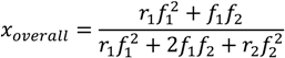
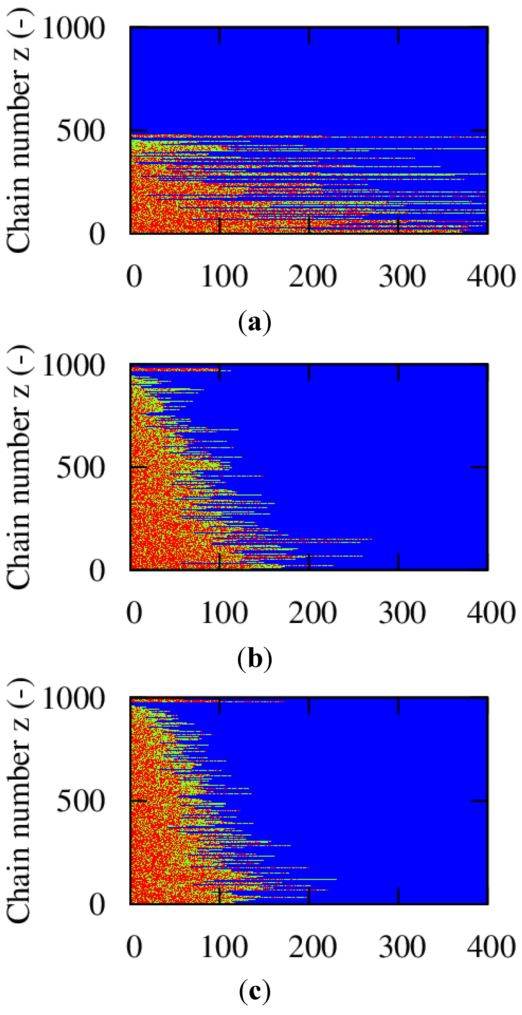
For a conversion of 0.90, the corresponding explicit monomer sequences are depicted in
Figure 2 (red unit: MMA unit; green unit:
nBuA unit) by selecting randomly a maximum number of 1000 copolymer chains out of the aforementioned 150,000 copolymer chains used for accurate <GD> calculation. Less than 1000 copolymer chains result, since incomplete ATRP initiation or termination by recombination can take place leading to the appearance of full horizontal blue dotted lines after the random selection procedure. In addition, in
Figure 2, a distinction is made between dormant and dead polymer chains with the latter type of chains shown in the top region of the polymer sample. Clearly, more well-defined (dormant) gradient copolymer molecules are obtained if a higher initial Cu(II) amount is selected. Higher Cu(II) amounts lead to a smoother transition of one comonomer type into the other comonomer type and to the formation of a higher amount of dormant chains, with additionally a more uniform chain length. Indeed, as confirmed in
Figure 3b–d, at high conversion, the lowest dispersity and highest EGF values are obtained in case a ppm level of 50 is used.
Figure 2.
Effect of initial Cu(II) ppm level ((
a): 10 ppm; (
b): 30 ppm; (
c): 50 ppm)) on the explicit copolymer composition at a conversion of 0.90 (conversion: comonomer 1 + 2); red: MMA unit; green:
nBuA unit; shown for representative kMC polymer sample (maximum of 1000 out of 150,000 chains); dead polymer chains and dormant polymer chains differentiated (top/bottom region); corresponding average properties (
xn, dispersity, EGF) specified in
Figure 3; 80 °C; [
M]
0:[
R0X]
0:[
I2]
0 = 100:1:0.02; AIBN; [
M1]
0 = [
M2]
0;
Table 1: intrinsic coefficients.
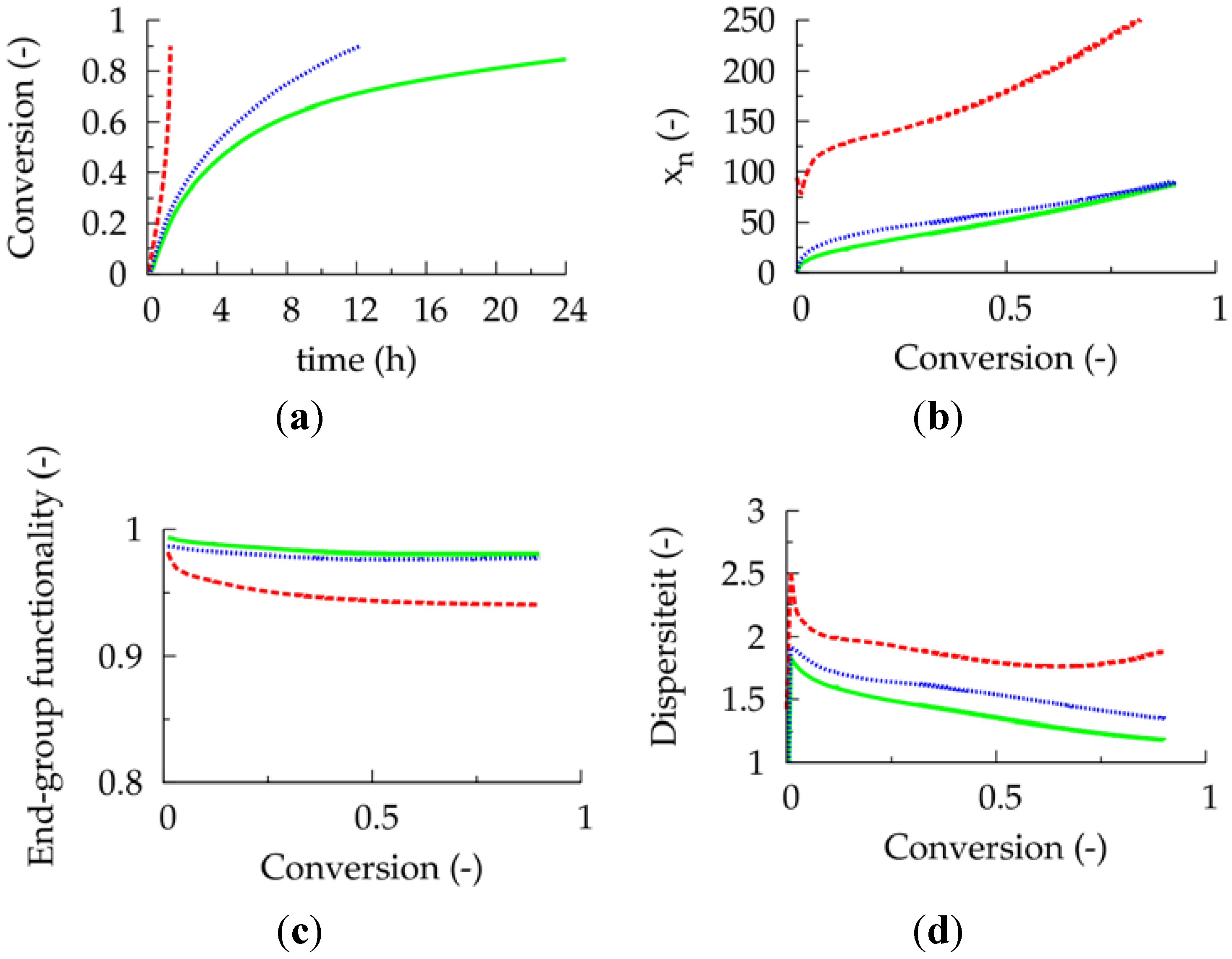
Unfortunately, at this higher initial Cu(II) ppm level the polymerization rate is much lower, as can be derived from
Figure 3a, which shows the effect of the initial Cu(II) ppm level on the conversion profile. To reach a conversion of 0.90 only 2 h are needed at 10 ppm, whereas already 16 h are required in case 50 ppm is employed. In agreement with previous deterministic simulations on ICAR ATRP homopolymerization [
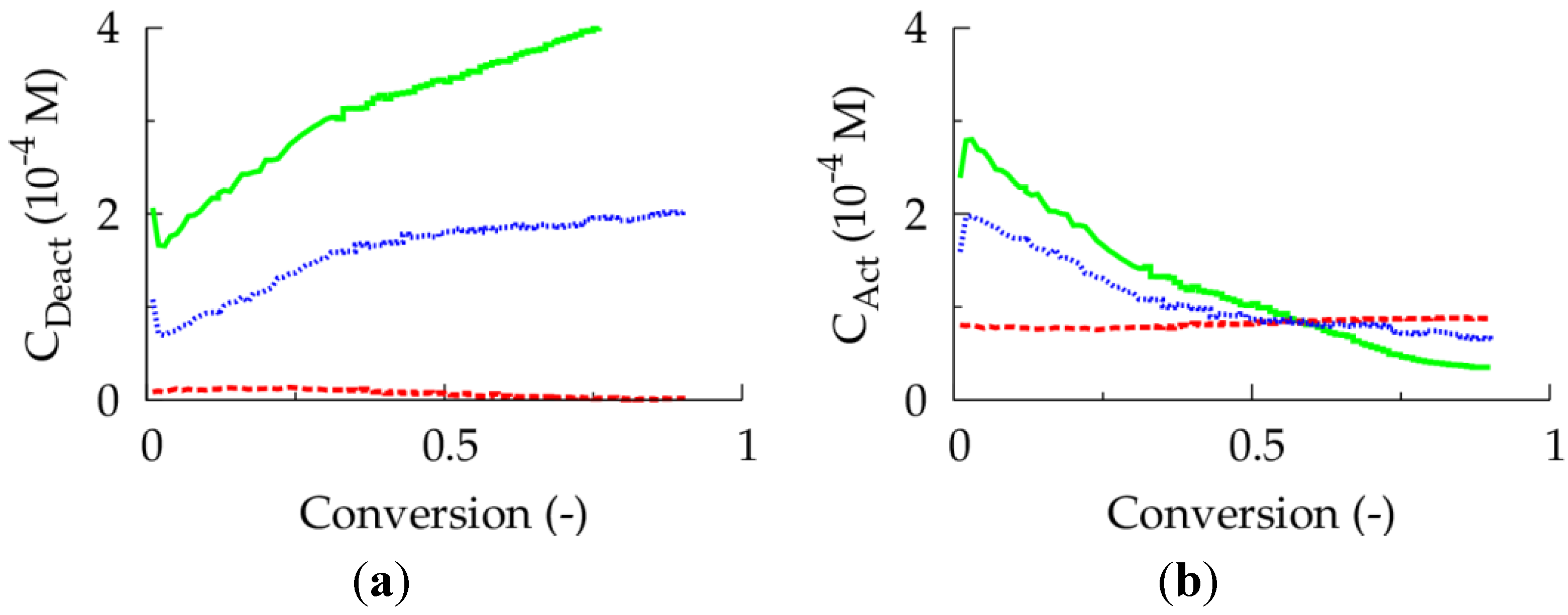
22], too low ppm levels lead to FRP behavior, as a sufficient amount of deactivator is needed to ensure controlled activation-growth-deactivation cycles. For an initial Cu(II) amount of 10 ppm, as shown in
Figure 4, the ATRP catalyst is mostly in its activator state and an almost zero deactivator concentration is obtained at high conversion. In contrast, for an initial Cu(II) ppm level of 50, a high amount of ATRP catalyst is always in the deactivator state allowing for control over chain length albeit at the expense of a strong reduction in polymerization rate.
In what follows, it is shown that a fed-batch procedure allows to accelerate the ICAR ATRP process without lowering the control over the copolymer microstructure. A distinction is made between ICAR ATRP processes in which a fed-batch addition procedure is applied for only one compound, namely the conventional radical initiator, and different compounds, i.e., not only the conventional radical initiator but also the comonomers and the deactivator are added in a fed-batch manner.
Figure 3.
(
a) Conversion as a function of polymerization time. (
b) Number average chain length (
xn) as a function of conversion. (
c) End-group functionality (EGF) as a function of conversion. (
d) Dispersity as a function of conversion; dashed red lines: 10 ppm; blue dotted lines: 30 ppm; full green lines: 50 ppm; 80 °C; [
M]
0:[
R0X]
0:[
I2]
0 = 100:1: 0.02; [
M1]
0 = [
M2]
0; conversion: comonomer 1 + 2 ;
Table 1: intrinsic coefficients.
Figure 4.
(
a) Deactivator concentration as a function of conversion. (
b) Activator concentration as a function of conversion;
![Polymers 06 01074 i027]()
: 10 ppm;
![Polymers 06 01074 i028]()
: 30 ppm;
![Polymers 06 01074 i029]()
: 50 ppm; 80 °C; [
M]
0:[
R0X]
0:[
I2]
0 = 100:1: 0.02; [
M1]
0 = [
M2]
0;
Table 1: intrinsic coefficients.
3.2. Fed-Batch Procedure for Addition of Conventional Radical Initiator
For a successful ICAR ATRP, the conventional radical initiator fragments formed upon dissociation, i.e., the I species, should allow for activator generation at the start of the polymerization and for activator regeneration later on in case termination reactions have lowered the radical concentration. Hence, the ideal I concentration profile can be calculated in silico by (i) starting the polymerization with very little I2 species, (ii) tracking explicitly the number of termination reactions in the kMC simulations and (iii) “adding” two I species each time termination occurs. However, in practice these I species have to be created through dissociation of a conventional radical initiator I2, which is characterized by a given half-life time. Hence, deviations from this desired concentration profile can be expected, even if a “cocktail” of I2 species would be used instead.
Based on simulations with this instantaneous “addition” of
I species, it fortunately follows for example that the continuous addition of a constant low
I2 amount throughout the ICAR ATRP allows to mimic the desired
I profile. In such simulations,
I2 is added in a dissolved form aiming at low overall change of the volume of the reaction medium (≪1 vol%). Typical pump flow rates for 1 mL syringes are applied as experimentally applied in literature [
37].
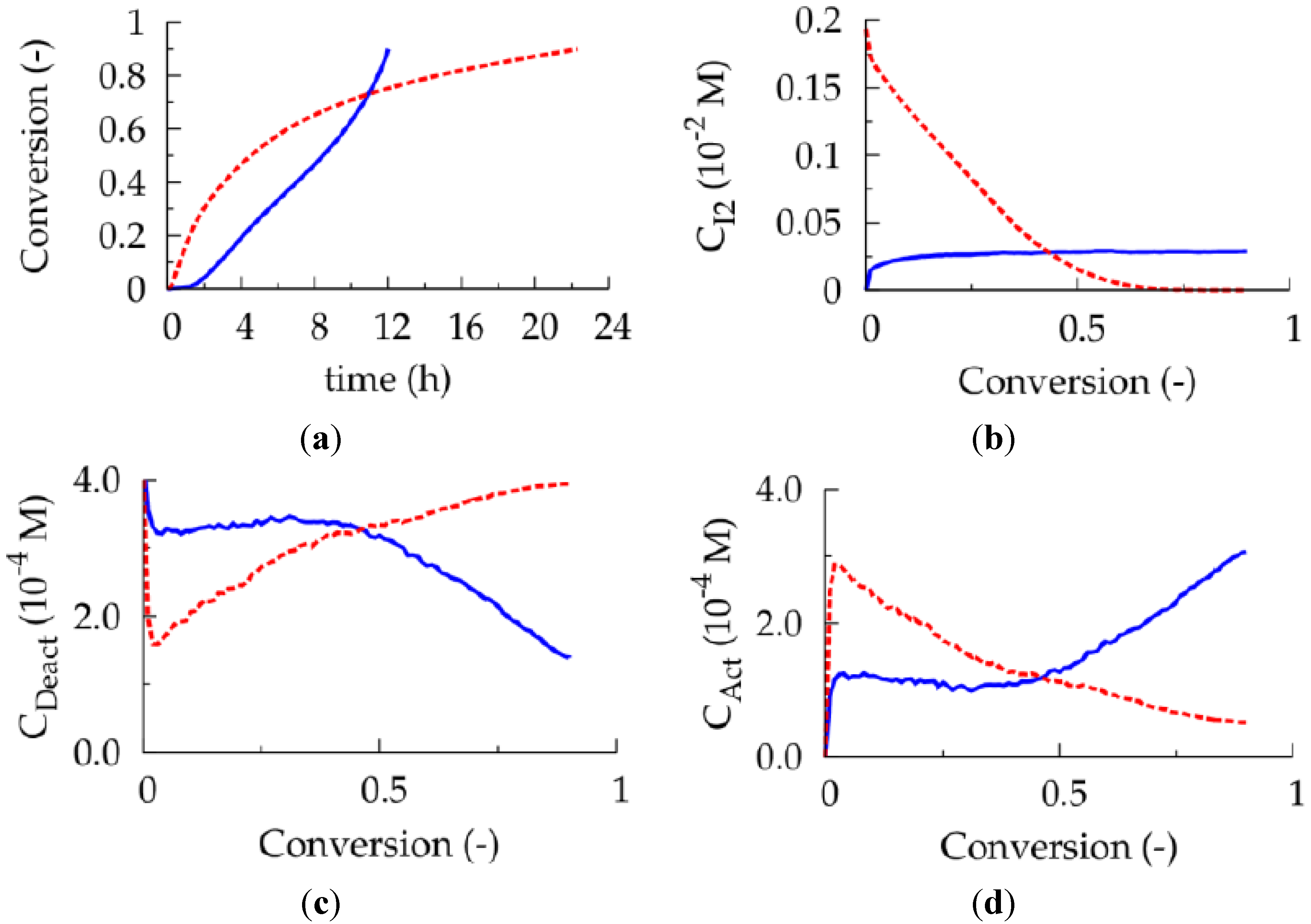
For an initial Cu(II) ppm level of 50 aiming at a conversion of 0.90, it is shown in
Figure 5a that such alternative fed-batch procedure (full blue lines; 80 °C; TCL = 100; per liter reaction mixture of the corresponding batch case 0.0017 μL dissolved
I2 added per second (concentration of
I2: 27 μmol L
−1)) allows for a lowering of the polymerization time compared to the corresponding batch ICAR ATRP. For the sake of comparison, in the batch case the total amount of
I2 added in the fed-batch procedure is present directly at the start of the polymerization (red dashed lines). Note that at low conversion the batch ICAR ATRP process is faster, as a higher conventional radical initiator concentration (
Figure 5b; dashed red versus full blue line) is obtained and thus a faster activator (re)generation (
Figure 5c,d; red dashed line versus full blue line) takes place. At high conversions, on the other hand, in the fed-batch ICAR ATRP process a higher
I2 concentration results leading to a lowering of the deactivator concentration and a polymerization rate acceleration. The net effect is a lowering of the number of termination events and, hence, a reduction of the overall polymerization time. Importantly, as illustrated in
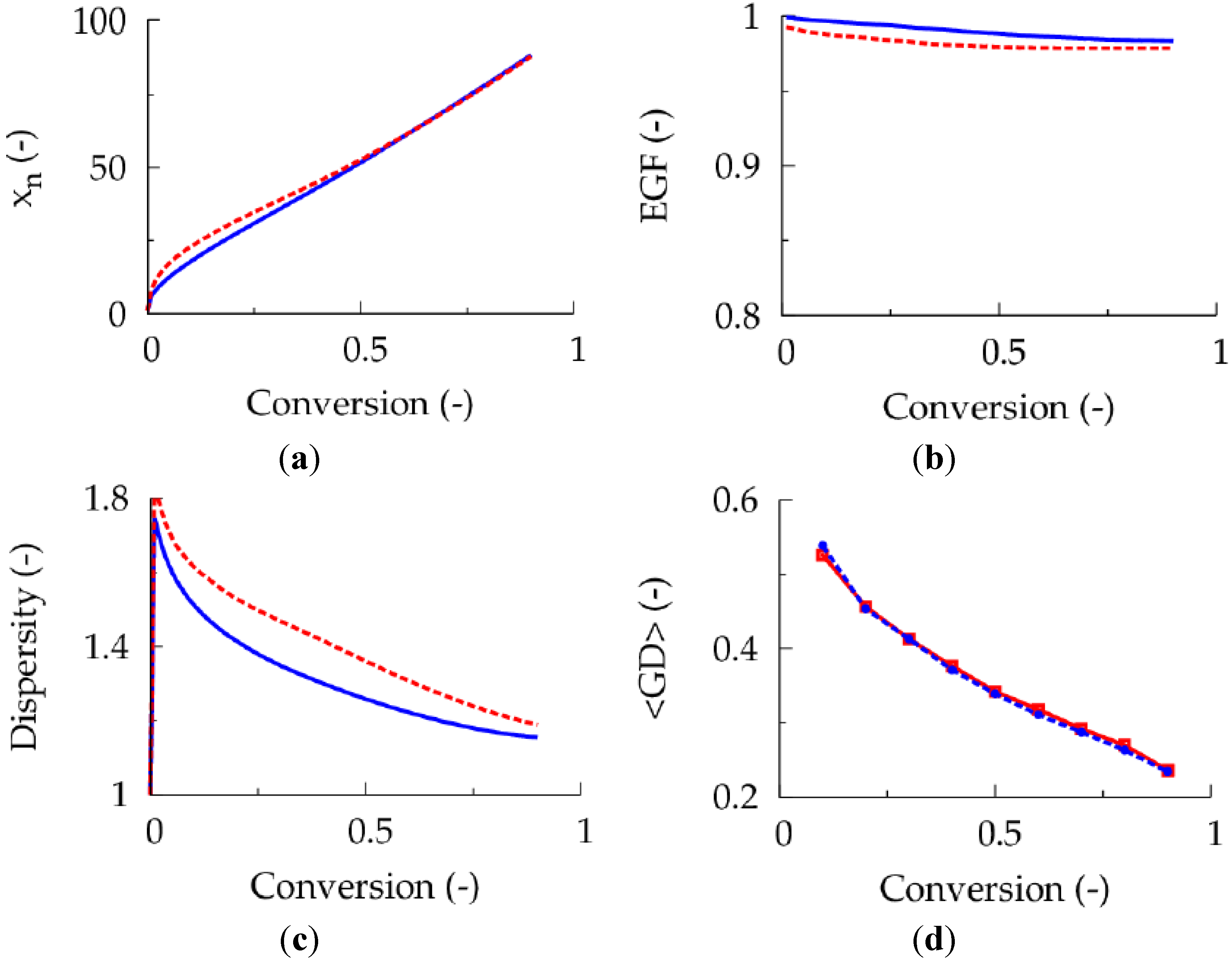
Figure 6 (blue dotted versus red dashed lines), this rate acceleration is not accompanied by a reduction of the control over polymer properties. As for the 50 ppm case, a <GD> value of
ca. 0.25 now results at high conversion implying a high linear gradient quality.
Figure 5.
(
a) Conversion as a function of polymerization time. (
b) Conventional radical initiator concentration as a function of conversion. (
c) Deactivator concentration as a function of conversion. (
d) Activator concentration as a function of conversion; common conditions: [
M]
0:[
R0X]
0 = 100:1, [
M1]
0 = [
M2]
0, and 50 ppm Cu(II) initially;
![Polymers 06 01074 i027]()
: batch [
I2]
0:[
R0X]
0 = 0.022 (same amount of
I2 as in fed-batch case up to a conversion of 0.90);
![Polymers 06 01074 i028]()
: fed-batch addition of dissolved
I2: 27 μmol·L
−1 with flow rate of 0.0017 μL s
−1 per liter reaction mixture of the corresponding batch case;
Table 1: intrinsic coefficients.
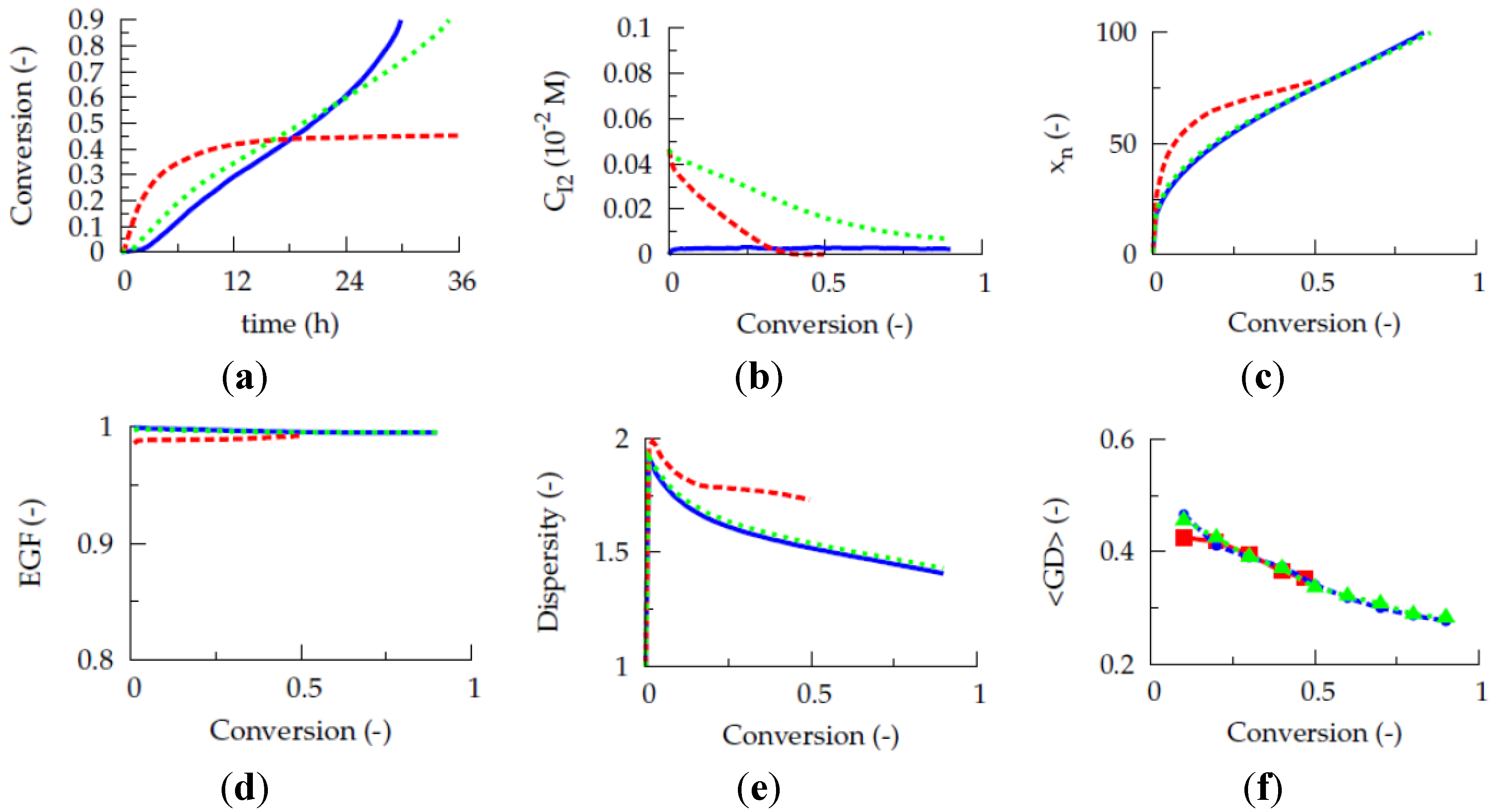
For a lower initial Cu(II) level of 10 ppm (80 °C; TCL = 100), the beneficial effect of a fed-batch approach for the addition of conventional radical initiator is even more pronounced. It follows from
Figure 7 that with this fed-batch procedure (full blue vs. dashed red lines), no rate retardation takes place guaranteeing a high conversion while keeping <GD> below 0.30. Note that compared to the 50 ppm case (
Figure 5 and
Figure 6) less
I2 is added in total ([
I2]
0:[
R0X]
0 = 0.022 versus [
I2]
0:[
R0X]
0 = 0.0052). As indicated above, to ensure a high control over the ICAR ATRP process FRP behavior has to be circumvented, explaining the lower
I2 amounts in case the initial Cu(II) ppm level is decreased. Such decrease implies, however, a relatively high overall polymerization time (30 h for a conversion of 0.90). Hence, it can be concluded that fed-batch addition of conventional radical initiator allows a more efficient synthesis of ICAR ATRP gradient copolymers in case a sufficiently low feeding rate is selected with respect to the desired Cu ppm level.
Figure 6.
(
a) Number average chain length (
xn) as a function of conversion. (
b) End-group functionality (EGF) as a function of conversion. (
c) Dispersity as a function of conversion. (
d) Gradient deviation (<GD>) as a function of conversion; common conditions: [
M]
0:[
R0X]
0 = 100:1, [
M1]
0 = [
M2]
0, and 50 ppm Cu(II) initially; batch: red dashed line; [AIBN]
0:[
R0X]
0 = 0.22 (same amount of
I2 in fed-batch case up to a conversion 0.90); full blue line: fed-batch addition of dissolved
I2: 27 μmol L
−1 I2 with flow rate of 0.0017 μL s
−1 per liter reaction mixture;
Table 1: intrinsic coefficients.
For completeness it is mentioned here that alternatively a conventional radical initiator characterized by a sufficiently high conventional radical initiator half-life time can be used under batch conditions. For example, as illustrated in
Figure 7 (green dotted lines; 10 times lower
kchem for dissociation than in
Table 1), a controlled supply of initiator radicals is then also obtained. Simulations revealed however that the fastest ICAR ATRP is still obtained using the fed-batch approach (blue lines), considering a wide range of half-life times.
Figure 7.
(
a) Conversion as a function of polymerization. (
b) Conventional radical initiator as a function of conversion. (
c) Number average chain length (
xn) as a function of conversion. (
d) End-group functionality (EGF) as a function of conversion. (
e) Dispersity as a function of conversion. (
f) Gradient deviation (<GD>) as a function of conversion; common conditions: [
M]
0:[
R0X]
0 = 100:1, [
M1]
0 = [
M2]
0, and 10 ppm Cu(II) initially; dashed red line: batch [
I2]
0:[
R0X]
0 = 0.0052 (same amount of
I2 as overall in fed-batch case up to a conversion of 0.90); full blue line: fed-batch addition of dissolved
I2: 2.7 μmol L
−1 I2 with flow rate of 0.0017 μL s
−1 per liter reaction mixture of the corresponding batch case; intrinsic rate coefficients:
Table 1; dotted green line: conditions as for dashed red line but with ten times lower value for dissociation rate coefficient than specified in
Table 1.
3.3. Multi-Component Fed-Batch Procedure for Addition of Conventional Radical Initiator, Comonomer, and Deactivator
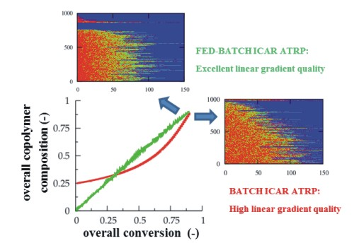
In the previous kMC simulations, the total amount of monomer was added completely before the ICAR ATRP was started. Under such conditions, a non-linear relation exists between
F1,inst and the monomer conversion (
Figure 1c). However, for a ‘perfect’ linear gradient polymer, it can be expected that a linear relation between
F1,inst and conversion according to the first bisector allows a better control over the monomer sequences toward the targeted linear gradient copolymer microstructure. In practice, the required monomer sequences can be obtained by adjusting in a fed-batch manner the comonomer feed composition through a variation of the added amount of comonomer.
In other words,
f1 should be altered
in situ so that after each addition
F1,inst is equal to the “overall monomer conversion
xoverall”, which is defined with respect to the total amount of monomer used in the corresponding
batch case:
In particular, when the instantaneous overall incorporation of both comonomers is equal (
F1,inst = 0.5), the “overall conversion” should be 0.5. In practice, the desired
f1 at a given
xoverall can be obtained based on the Mayo-Lewis equation (Equation (1)) and noting that
f2 is equal to 1−
f1:
For “normal” ATRP [
38] and RAFT polymerization [
39], such Mayo-Lewis based fed-batch additions were already explored with computer simulations, while assessing the overall conversion based on the number average chain length,
i.e., assuming controlled conditions, and considering a monomer feed policy in which all of the less reactive comonomer is initially present and only the more reactive comonomer is added along the polymerization. However, in these kinetic studies, in which no explicit calculation of the copolymer composition is included, the fed/semi-batch addition of comonomer is accompanied by a low polymerization rate, a rather high dispersity and a relatively low livingness. As indicated in a recent kMC study of Van Steenberge
et al. [
26] low dipersities are required for controlled linear gradient synthesis and it can therefore be expected that under the reported literature conditions still relatively high <GD> values are obtained, despite the linear relation between
F1,inst and
xoverall.
In this work, the ICAR ATRP fed-batch conditions are carefully selected to minimize the negative tendencies reported for related CRP systems [
38,
39]. First of all, simulations revealed that it is most suited to start the ICAR ATRP with a low monomer amount and add frequently small amounts of both comonomers under starved-feed conditions,
i.e., at a constant high
in situ conversion (e.g., >0.85) small amounts of both comonomers should be added in order to control the number of monomers added in between a single activation and deactivation. The use of starved-feed conditions is a common procedure in FRP processes with the beneficial safety effect in the case of a sudden loss of cooling capacity [
40].
To guarantee a good control over chain length a predefined Cu level is also required taking into account the volume increase of the reaction medium upon fed-batch monomer addition. Hence, deactivator has to be added along the ICAR ATRP process as well. For a direct comparison with the batch condition, it is most suited to add deactivator so that a fixed ppm level of Cu is obtained with respect to the amount of monomer that has been added until the considered time, i.e., calculating the deactivator supply rate based on both the amount of monomer in the monomer feed and the amount of monomer already incorporated in the copolymer chains. In what follows, double quotation marks are used to differentiate such ppm levels from the aforementioned ppm levels. For completeness, it is mentioned here that initially the volume of the ATRP initiator cannot be neglected in these simulations.
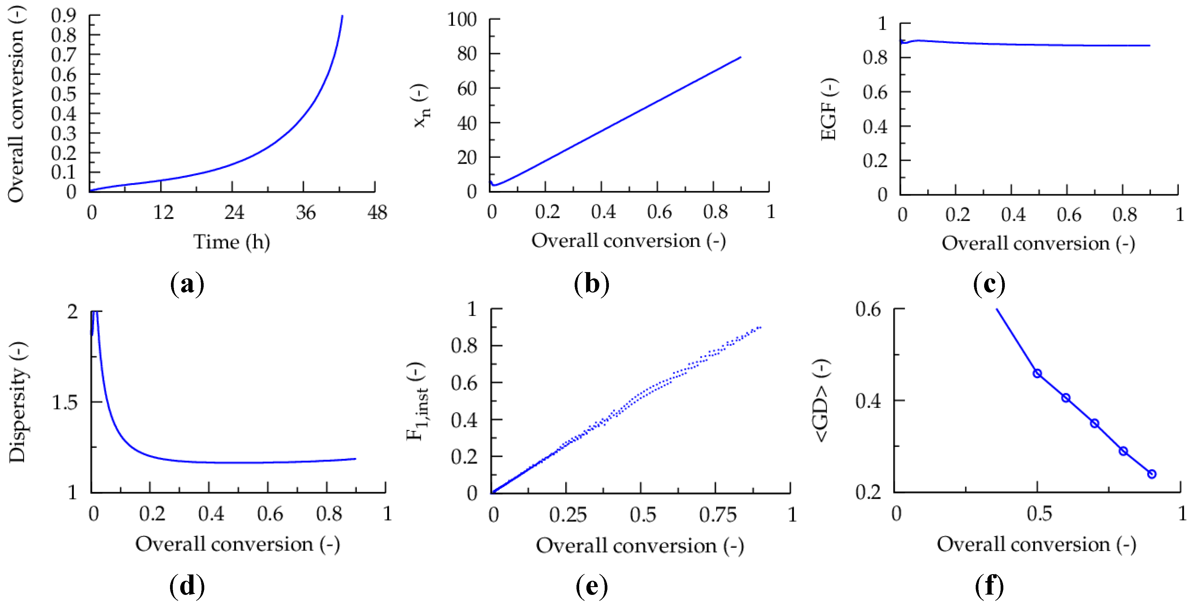
In case a high
in situ monomer conversion of 0.90,
i.e., 90% conversion with respect to the cumulative amount of monomer added, is demanded prior to each fed-batch monomer addition, a high gradient quality (<GD> of
ca. 0.20) can be obtained, as illustrated in
Figure 8. For these figures, one percentage of the total amount of monomer of the batch counterpart is added initially in pure MMA form and dissolved conventional radical initiator is added continuously (per liter reaction mixture of the corresponding batch case: 0.0017 μL dissolved
I2 added per second (concentration
I2: 27 μmol L
−1).
Figure 8.
(
a) Overall conversion (based on monomer amount of corresponding batch case; Equation (2): as a function of polymerization. (
b) Number average chain length (
xn) as a function of overall conversion. (
c) End-group functionality (EGF) as a function of overall conversion. (
d) Dispersity as a function of overall conversion. (
e) Evolution of instantaneous copolymer composition (
F1,inst) as a function of the overall conversion. (
f) Gradient deviation (<GD>) as a function of conversion; initial conditions: TCL = 100 (in case all monomer would be added instantaneously), and 50 ppm Cu(II); fed-batch addition of dissolved
I2: 27 μmol L
−1 with flow rate of 0.001 μL s
−1 per liter reaction mixture of the corresponding batch case; fed-batch addition of comonomer based on Equation (3) each time an
in situ conversion of 0.9 is reached (with at the start 1% of the batch amount in pure MMA form); comonomer addition accompanied by addition of deactivator so that Cu level is again “50 ppm (with respect to the monomer and monomer units)”;
Table 1: intrinsic coefficients.
![Polymers 06 01074 g008]()
Per addition step, the comonomer molar ratio is adjusted based on Equation (3) so that
F1,inst varies linearly with the overall monomer conversion. Furthermore, throughout this ICAR ATRP a Cu level of “50 ppm” is imposed by addition of deactivator each time monomer is added. A total number of
ca. fifty-five fed-batch additions results, corresponding to an almost negligible drop of the
in situ monomer conversion upon each monomer addition, implying that the linear gradient microstructure is synthesized via very stable activation-growth-deactivation cycles. Note that the polymerization is conducted already under viscous conditions at low polymerization times, a similar strategy as followed by Bentein
et al. [
41] in their work on the optimization of nitroxide mediated polymerization of styrene.
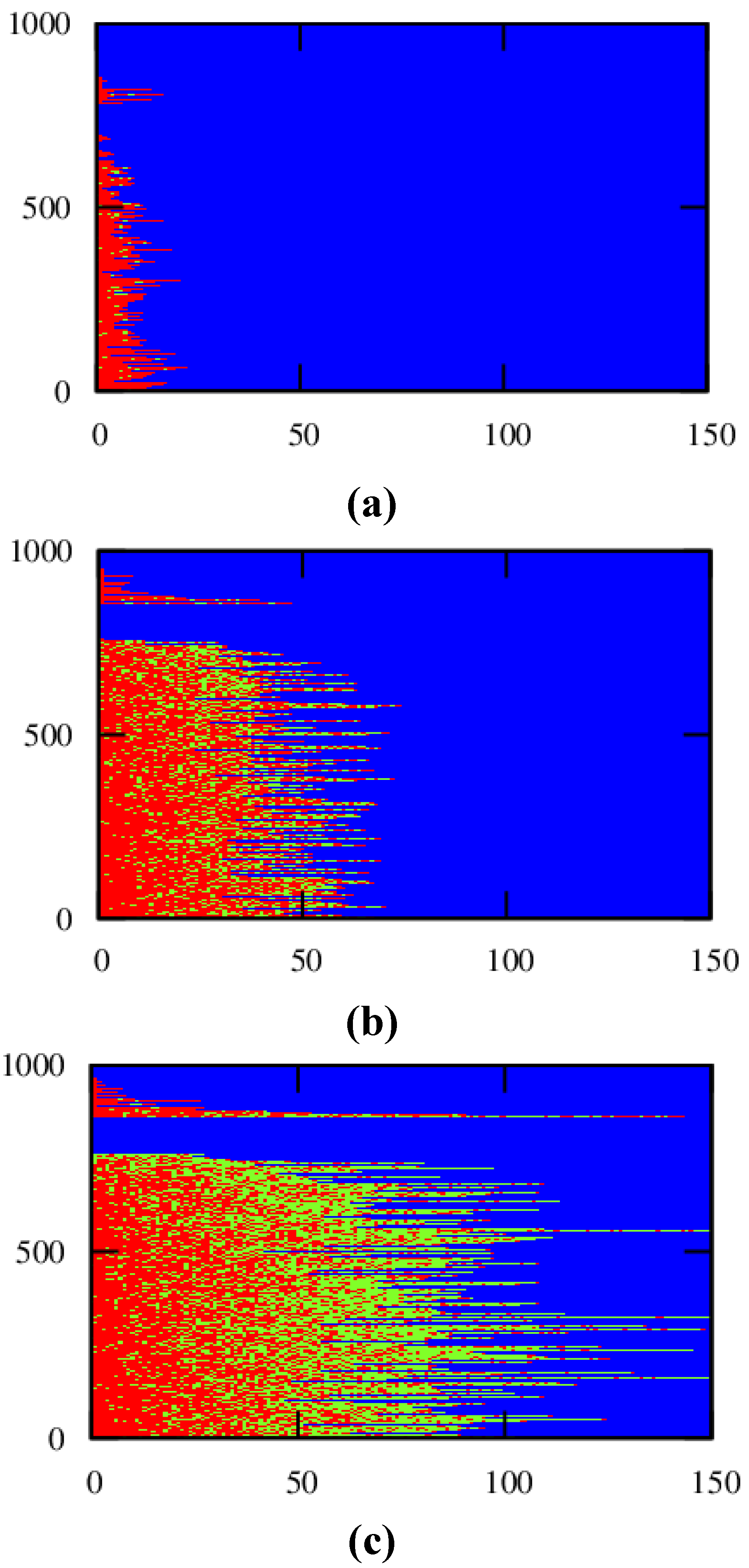
The high linear gradient quality is confirmed in
Figure 9, which shows the corresponding explicit copolymer compositions at an overall conversion of 0.10, 0.50 and 0.90. Importantly, under the studied conditions, at very low overall conversions now almost exclusively MMA (red) units are incorporated, which is a direct consequence of the monomer feed batch policy (
Figure 8e versus
Figure 1c). Clearly, the dormant copolymer chains possess a much higher linear gradient quality (e.g.,
Figure 9 versus
Figure 2). Note that it can be expected that the oligomeric dead polymer molecules will be washed out upon polymer isolation and thus a polymer product with a very high gradient quality is obtained, underlining the potential of the multi-component fed-batch technique with respect to control over monomer sequences.
Figure 9.
Explicit copolymer composition using multi-component fed-batch procedure at a conversion of (
a) 0.10, (
b) 0.50 and (
c) 0.90; red: MMA unit; green:
nBuA unit; shown for representative kMC polymer sample; dead polymer chains and dormant polymer chains differentiated (top/bottom region); conditions: see caption of
Figure 8; overall conversion: Equation (2): with respect to batch case;
Table 1: intrinsic coefficients.
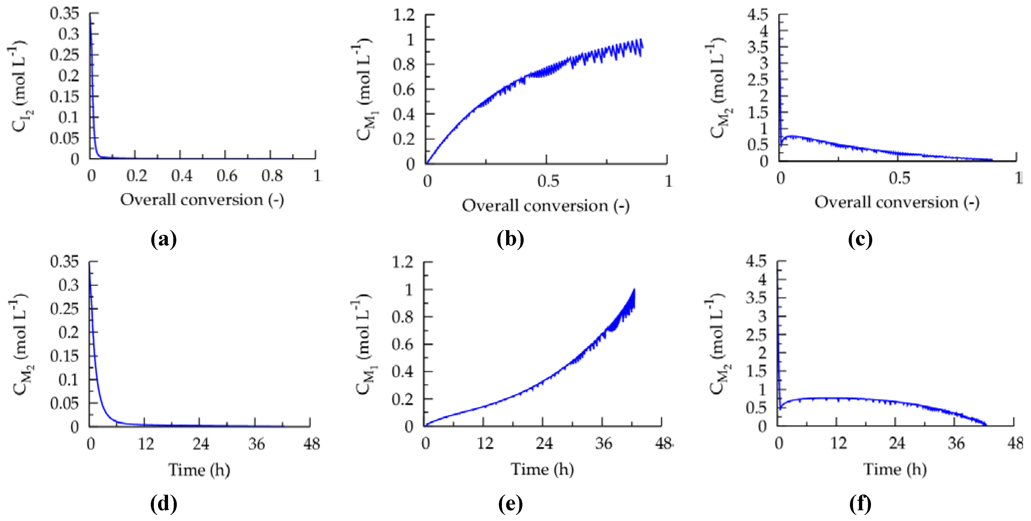
The corresponding evolutions of the comonomer concentrations and concentration of the conventional radical initiator with the overall conversion and polymerization time are given in
Figure 10. It can be seen that along the ICAR ATRP the monomer feed is enriched with
nBuA (monomer 1), as requested for MMA-
nBuA linear gradient formation. Initially, the conventional radical initiator concentration is high to ensure good activator regeneration. At higher conversions, this concentration drops, due to the volume increase upon monomer addition, and FRP behavior is thus circumvented leading to a good control over polymer properties. However, despite this excellent control, a relatively slow ICAR ATRP is obtained, in agreement with literature reports on related CRP systems [
38,
39].
Figure 10.
(
a) Conventional radical initiator as a function of overall conversion. (
b) Comonomer concentrations as a function of overall conversion. (
d–f) Corresponding subfigures for (
a–c) when expressed as a function of time; conditions: see caption of
Figure 8; overall conversion: Equation (2): with respect to batch case;
Table 1: intrinsic coefficients.
It can thus be concluded that the highest linear gradient quality can be obtained using a multi-component fed-batch approach, as it allows tailor-design of linear gradient dormant copolymer chains albeit at the expense of an increase of the polymerization time.


 : 10 ppm;
  : 30 ppm;
  : 50 ppm; also included in (b) as -- -- : Mayo-Lewis equation (Equation (1)); conversion: comonomer 1 + 2; Table 1: intrinsic coefficients.