Review

Challenges in Multiscale Modeling of Polymer Dynamics

1
Department of Mechanical Engineering, Northwestern University, Evanston, IL 60208, USA
2
Theoretical & Applied Mechanics, Northwestern University, Evanston, IL 60208, USA
3
Department of Materials, Polymer Physics, ETH Zurich, CH-8093 Zurich, Switzerland
*
Author to whom correspondence should be addressed.
Visiting Distinguished Professor of Mechanical Engineering, World Class University Program in Sungkyunkwan University, Korea
Adjunct Professor under the Distinguished Scientists Program Committee at King Abdulaziz University (KAU), Jeddah, Saudi Arabia
Polymers 2013, 5(2), 751-832; https://doi.org/10.3390/polym5020751
Submission received: 3 April 2013 / Revised: 16 May 2013 / Accepted: 30 May 2013 / Published: 13 June 2013
(This article belongs to the Special Issue Multiscale Simulations in Soft Matter)

Abstract

:
The mechanical and physical properties of polymeric materials originate from the interplay of phenomena at different spatial and temporal scales. As such, it is necessary to adopt multiscale techniques when modeling polymeric materials in order to account for all important mechanisms. Over the past two decades, a number of different multiscale computational techniques have been developed that can be divided into three categories: (i) coarse-graining methods for generic polymers; (ii) systematic coarse-graining methods and (iii) multiple-scale-bridging methods. In this work, we discuss and compare eleven different multiscale computational techniques falling under these categories and assess them critically according to their ability to provide a rigorous link between polymer chemistry and rheological material properties. For each technique, the fundamental ideas and equations are introduced, and the most important results or predictions are shown and discussed. On the one hand, this review provides a comprehensive tutorial on multiscale computational techniques, which will be of interest to readers newly entering this field; on the other, it presents a critical discussion of the future opportunities and key challenges in the multiscale modeling of polymeric materials and how these methods can help us to optimize and design new polymeric materials.

Graphical Abstract

1. Introduction

The design and processing of polymeric materials become increasingly difficult as performance requirements of many advanced technological applications become stricter, and as the demand increases for shorter ideation-to-implementation times. It is therefore of great interest to predict and design the key physical and mechanical properties of polymeric materials from information about molecular ingredients. Consequently, it is important to establish a rigorous link between molecular constituents and macroscopic mechanical properties, i.e., between polymer chemistry and viscoelasticity, in particular. With such a tool at hand, the optimal processing, design and application of polymeric materials can be more easily realized. However, establishing such a rigorous link is not a simple task, and it has not yet been fully achieved. The difficulty arises from the wide range of spatial and temporal scales involved in the characterization of polymeric materials (in contrast to, for example, the case of a monoatomic gas), as illustrated in Figure 1. The typical vibrations of covalent bonds are on the length scale of an Ångström and time scale of sub-picoseconds. The typical length of a monomer is a nanometer, with relevant dynamics in the range of tens of picoseconds. The size of a single polymer chain is characterized by its radius of gyration, typically between 10 and 100 nanometers. Depending on its surroundings, the relaxation of a single chain lasts about 10 to 100 nanoseconds, but often longer. Beyond a critical concentration, different polymer chains are coiled together with mutual uncrossability. A typical polymeric network has a size of about 1 to 100 micrometers, with a relaxation time on the order of microseconds to milliseconds. Bulk polymeric material is composed of these coils and networks on the length scale of millimeters to centimeters. The relaxation and aging of these bulk polymeric materials occur in the range of seconds, hours and even years. These multiple, disparate spatial and temporal scales and their interdependence among each other in terms of system behavior (i.e., bulk behavior depends on the behavior of individual polymer chains, and so forth) make it necessary to adopt a multiscale modeling technique that can correctly characterize the hierarchy of scales, if we wish to link molecular constituents with macroscopic mechanical properties, including viscoelasticity, viscoplasticity and aging of rubbery or glassy polymers. It is not feasible to review the multiscale modeling of all of these properties in this work; instead, we focus on the viscoelasticity (rheological properties) of polymer melts, which is one of the most important issues in the processing, molding and application performance of polymeric materials. We begin by discussing the cause of viscoelastic behavior in polymer melts.
Figure 1. Hierarchical length scales for polymeric materials.
Polymers 05 00751 g001
The viscosity of polymeric materials originates from the dynamics of polymer chains. If the chains are very short, i.e., they are oligomers; their dynamics are dominated by the friction between monomers. According to the Rouse theory, the viscosity, η 0 , of these oligomers has a simple scaling relationship with chain length N, as η 0 N , and the self-diffusion coefficient scales as D cm N - 1 [1]. These phenomena have also been observed both in molecular dynamics (MD) simulations [2,3] and experiments [4]. However, when the chain length is larger than the entanglement length ( N > N e ), due to chain connectivity and uncrossability, the dynamics of these long chains will be greatly hindered by topological constraints, referred to as entanglements. These entanglements are commonly assumed to effectively restrict the lateral motion of individual polymer chains into a tube-like region with diameter a pp . Thus, a chain will slither back and forth, or reptate, along the tube, instead of moving randomly through three dimensional space. When the time, t, is shorter than the entanglement time, τ e , the chain does not feel the constraints of the tube formed by its neighboring chains. Thus, it can move isotropically in space. At intermediate times, τ e < t < τ R , the chain segments move along the axis of the tube in a Rouse-like fashion, where τ R is the Rouse time, and only the two ends of the polymer chain explore new space. The inner segments of the chain behave like a random walk inside the tube [5]. Beyond the Rouse time ( τ R < t < τ d ), the chain moves inside the tube in a one-dimensional diffusive manner, where τ d is the disentanglement time. At longer times ( t > τ d ), the chain can completely escape its original tube and form a new tube with its neighboring chains. This picture for entangled polymer chain dynamics constitutes the so-called tube model, the most successful theory from the field of polymer physics in the past thirty years. The central axis of the tube-like region defines the primitive path (PP). The PP can be considered as the shortest path remaining, if one holds the two ends of the chain in space and continuously shrinks its contour without violation of the chain’s uncrossability with its neighboring chains. De Gennes [5] and Doi and Edwards [6] performed the pioneering works on the theoretical study of rheological properties of entangled polymer melts following from the tube concept. The dynamics of entangled polymer chains was considered in terms of the one-dimensional diffusion of a tracer chain along its PP in a mean-field approach (i.e., the constraints formed by neighboring chains are considered static). The PP was treated as a random walk in space with a constant step length, a pp . Thus, the degree of the topological interactions between different chains is also defined through the effective tube diameter, a pp . From the tube theory [5,6], D cm N - 2 and η 0 N 3 , which agree reasonably well with the experimental observations. Later on, two important mechanisms observed in real polymer systems, contour length fluctuation (CLF) and constraint release (CR), were subsequently incorporated into the tube theory, which then predicts η 0 N 3.4 [7]. In the original tube theory, the contour length of the chain was assumed to remain fixed at the mean value, L, when in actuality, it fluctuates about this mean value with root-mean-squared fluctuation on the order of δ L L ( N e / N ) 1 / 2 [8] and, thus, manifests itself in the dynamics of moderately long chains, but becomes negligible for extremely long chains. In addition, the motion of surrounding chains can release lateral constraints to the motion of the tracer chain, thereby dilating or otherwise reorganizing its surrounding tube. Thus, CR is a cooperative phenomenon between different chains, while CLF can be considered as a single-chain phenomenon, but both hasten the relaxation process. By taking these important mechanisms into account, various models have been developed [7,8,9,10,11,12,13], which result in significant improvements when compared with experimental results. In particular, Likhtman and McLeish [14] developed a quantitative theory for the linear dynamics of linear entangled polymers with all the relevant mechanisms considered, i.e., CLF, CR and longitudinal stress relaxation along the tube. Later on, Hou et al. [15] performed extensive simulations of the stress relaxation of bead-spring polymers. They found that their simulation results agreed with the Likhtman-McLeish theory [14] by using the double reptation approximation for the CR effect and removing high-frequency CLF contributions [15]. The related theories have also been extensively reviewed in the literature [7,10,11,12,13,16,17,18,19,20].
Since about 90% of the free energy of polymeric materials is entropy [21], the elasticity of these materials is dominated by entropic forces whose strength is inversely proportional to k B T , where k B is Boltzmann’s constant and T denotes absolute temperature. To explore why the elastic modulus of rubber eventually becomes independent of the strand length in the network, Edwards invented the tube concept in his description of rubber elasticity [22,23,24]. De Gennes then realized that one can omit the crosslinks when the chains become very long, and he adopted the tube concept to study the polymer chain reptation inside a strongly crosslinked polymeric gel [25]. Later on, through rigorous statistical mechanic formulations, upon employing the affine deformation assumption, Edwards and Vilgis established the contributions of entanglements and crosslinks to the elastic response of a crosslinked network following an external applied force [21]. The obtained results compared well with the extensive experimental results. Rubinstein and Panyukov [26] adopted a similar idea to establish an affine length scale, R aff , which separates the deformation of polymer networks into two regimes: the solid, elastic, affine deformation on large scales and the liquid-like nonaffine deformation on smaller scales. They also demonstrated that the nonlinear elasticity of polymer networks is induced by nonaffine deformation [26]. The proposed method also unified the phantom (crosslinked) and entangled networks and lead to a simple stress-strain relationship for polymer networks, which has been further validated by experiments [26]. Later on, Rubinstein and Panyukov [27] combined and generalized several successful ideas into a new molecular model for the nonlinear elasticity of polymer networks, with the concepts of the tube model, CLF and CR mechanisms. The prediction of the new model agreed with experimental and computer-simulation results [27]. Arruda and Boyce [28] also developed a constitutive model for the nonlinear elasticity of rubber materials. In their model, the underlying structure of rubber materials is simplified into an eight-chain crosslinked cube, with each chain having Langevin (non-Gaussian) behavior. The proposed model successfully captures the response of real polymeric materials under uniaxial tension, biaxial extension, uniaxial compression and pure shear.
Having understood the origins of elasticity and viscosity, it was only a technical challenge to develop theoretical and thermodynamically consistent constitutive models for the viscoelasticity of polymeric materials, with all the relevant physical mechanisms considered [19,29,30,31,32,33]. However, the predictions and/or assumptions made in these theoretical models should be checked against computer simulations and experimental observations, to either accept, reject or refine the models as a whole or subsets of their basic assumptions. As accurate MD potentials are developed for a broad range of materials based on quantum chemistry calculations and with the increase of supercomputer performance, all-atomistic MD simulation has become a very powerful tool for analyzing the complex physical phenomena of polymeric materials, including dynamics, viscosity, shear thinning and α- and β-relaxations. However, as discussed above and illustrated in Figure 1, the interactions between different polymer chains are characterized by a wide range of spatial and temporal scales. It is still not feasible to perform all-atomistic MD simulations of highly entangled polymer chain systems, due to their large equilibration and relaxation times, long-range electrostatic interactions and tremendous number of atoms. The all-atomistic MD model for such a system, with a typical size of about a micrometer and a relaxation time on the scale of microseconds, would consist of billions of atoms and would require billions of time steps to run, which is obviously beyond the capability of the technique, even with the most sophisticated supercomputers available today. One of the largest united atom MD simulations (with hydrogen atoms ignored in the all-atomistic model) was done by Gee et al. [34] on spinodal decomposition preceding polymer crystallization. They simulated polyethylene (PE) polymer with a chain length of N = 384 and 4,478,976 united atoms in total, taking about ∼1 × 10 6 processor hours for a ∼50 ns simulation using 2048 processors. There is a huge demand to extend the approachable scales of all-atomistic simulations to the scales of real polymeric materials, with the help of multiscale computational techniques. With this ability, a rigorous link between the molecular compositions and macroscopic properties can be established to provide a powerful tool for optimizing the processing, design and application of polymeric materials.
Multiscale modeling techniques will play an important role in this process of verifying new and existing models, but also in guiding theoretical development and exploring unexpected physical phenomena. There exist some excellent and recent reviews on the coarse-graining of entangled polymers, focusing on static properties [35,36,37], dynamic properties [38,39,40,41] and the comparison between different systematic coarse-graining methods [42,43]. There are also several books on multiscale modeling of polymers and biomolecules [35,44,45,46,47,48], which cover particular methods not captured in this review. However, to our knowledge, there is no systematic review on the different multiscale modeling techniques developed in the past twenty years. This review attempts to provide an up-to-date overview of multiscale modeling methods within this time period, including current work. We will introduce the fundamental ideas and equations for each multiscale modeling method, and we will summarize key results. At the same time, this review may serve as a comprehensive tutorial for different multiscale computational techniques to those readers who are new in this field.
Self-consistent field theoretical approaches have been excluded from this review, because the underlying principles were established and developed more than two decades ago [49,50,51,52]. Still, a number of important applications were newly added in the recent past, including block copolymers and nanocomposites [53]; screening effects in polyelectrolyte brushes [54]; mixed polymer brushes [55]; harvesting cells cultured on thermoresponsive polymer brushes [56,57]; morphology control of hairy nanopores [58]; and the effect of charge, hydrophobicity and sequence of nucleoporins on the translocation of model particles through the nuclear pore complex [59]; to mention a few.
Another topic in multiscale modeling concerns the bridging of detailed ab-initio or density functional theory (DFT) calculations to the classical all-atomistic simulations. These methods provide the solid molecular scale foundations for the multiscale modeling method discussed in this review. However, these methods are beyond the scope of the current review. We recommend [60,61,62,63] and the references therein to the interested reader.
Yet another important topic is polymer mixtures. In polymer mixtures, different components are typically not miscible microscopically, because the entropy of mixing for polymers is smaller than that of small molecules. Therefore, a polymer mixture often separates into different phases, in which one of the polymer components is enriched. The simulation of such complex systems is a challenge involving additional complexities [64,65]. Due to the different modes of motion and relaxation for each component, the multiscale modeling of polymer mixtures and their structure formation, phase transition and inhomogeneity at equilibrium are computationally expensive, not even to speak of non-equilibrium. One of the most powerful methods to study polymer mixtures at equilibrium in an approximate manner is self-consistent field theory [66]. Some of the multiscale modeling methods reviewed in this paper have been extended to study polymer mixtures [67,68,69,70,71,72,73,74,75]. Interested readers may refer to these papers for details. Due to space limitations, this review sets out to put its focus on the multiscale modeling of homopolymers, while briefly mentioning extensions for mixtures.
This review is organized as follows. In Section 2, we give an overview of the different multiscale computational techniques and divide them into three categories. Section 3 introduces the different methods in the coarse-graining of generic polymers. Section 4 discusses systematic coarse-graining methods, from lightly or moderately coarse-grained models to highly coarse-grained ones where the whole polymer chain is lumped into a soft colloid. Section 5 reviews different multiple-scale-bridging methods developed in the past five years, which have distinct features compared with other methods. None of the latter methods have apparently been reviewed and compared in the literature. In Section 6, we discuss the perspectives and key challenges in the multiscale modeling of polymeric materials. Finally, we summarize and conclude in Section 7.

2. Overview of Multiscale Modeling Techniques

In this review, according to their capabilities, we divide different multiscale computational techniques into three categories: (i) coarse-graining methods for generic polymers; (ii) systematic coarse-graining methods and (iii) multiple-scale-bridging methods, as tabulated in Table 1. Methods falling into Category (i) mainly focus on the large scale simulation of generic polymers. The molecular details are ignored in this method below the scale of Kuhn or entanglement length. Large spatial and temporal scales can rather easily be approached by these generic methods, compared with all-atomistic MD simulations. Scaling laws characterizing the effect of molecular weight on the dynamics or rheology can be obtained and compared with the prediction from the Rouse or tube model, as well as with experiments [76]. However, since these methods neglect chemical details, the obtained results are usually difficult to compare with specific polymers. In contrast, in Category (ii), we review systemic coarse-graining methods, which can extend the approachable length and time scales of all-atomistic MD simulations, while keeping many intrinsic chemical and physical features of specific polymers, such as end-to-end distance, radius of gyration, diffusion coefficient and glass-transition temperature. Thus, the obtained results can be directly compared with experiments. According to the degree of coarse-graining, the systemic coarse-graining methods can be further divided into several models: the Iterative Boltzmann Inversion (IBI) method, the blob model and the super coarse-graining method. In the IBI method, one or two monomers are coarse-grained into one super atom. Within the blob model, ten to twenty monomers are coarse-grained into one blob. Within the super coarse-graining method, the whole chain is mapped to a single soft colloid. The approachable length and time scales of the MD simulations increase with the degree of coarse-graining. However, there are different issues involved in these methods, which we will discuss in this review. Finally, in category (iii), we discuss multiple-scale-bridging methods, which have been developed in the past five years. These methods have distinct features and develop different bridging laws for different scales, compared with the methods in other categories. These methods also overcome the unapproachable scales and phenomena in past simulations of polymeric materials and represent the frontier of multiscale modeling of polymeric materials. A comparison between different multiscale modeling methods is presented in Table 2.
Table 1. Summary of the methods discussed in this review.
CategoryMethodKey referencesGoverning formulation
(i)Bond-fluctuation method[67,77] Section 3.1Monte Carlo
(i)Finite-extensible non-linear elastic (FENE) Model[78,79] Section 3.2molecular dynamics (MD)
(i)Slip link model[80,81] Section 3.3MD
(ii)Iterative Boltzmann Inversion method[82,83] Section 4.1MD
(ii)Blob model[84,85] Section 4.2MD
(ii)Numerical super coarse-graining method[86] Section 4.3MD
(ii)Analytical super coarse-graining method[87,88] Section 4.3MD
(iii)Dynamic mapping onto tube model[89] Section 5.1MD and primitive path (PP) analysis
(iii)Molecularly-derived constitutive equation[90] Section 5.2MD and continuum model
(iii)Concurrent modeling of polymer melts[91] Section 5.3MD and continuum model
(iii)Hierarchical modeling of polymer rheology[92] Section 5.4MD, PP analysis and continuum model
Table 2. Comparison of the methods discussed in this review. D cm is the self-diffusion coefficient. G and G are the storage and loss moduli, respectively. G ( t ) and η denote the shear relaxation modulus and viscosity, respectively. The approachable temporal and spatial scales vary with the computer platform and the number of processors used. The acceleration of different multiscale modeling methods is estimated by taking the all-atomistic method as a baseline. Note that the bond-fluctuation method, FENE model and slip link model in Category (i) can only be applied to study generic polymers, not specific polymers. Here, D cm in the bond-fluctuation model is obtained based on the Monte Carlo (MC) step, not the real time. All the approachable temporal and spatial scales are estimated according to the time step and efficiency of the different methods, without considering the time-temperature superposition principle. This is the only multiscale modeling method developed so far, which can be applied to study both small and large deformation of polymeric materials for engineering applications.
CategoryMethodApproachable temporal and spatial scalesPredictable properties in the approachable scalesAcceleration
All-atomistic method 10 - 8 s and 10 - 8 m D cm , G , G , G ( t ) , η 1 ×
(i)Bond-fluctuation model 10 - 6 m and no time scale D cm N/A
(i)FENE model 10 - 6 s and 10 - 6 m D cm , G , G , G ( t ) , ηN/A
(i)Slip link model 10 - 5 s and 10 - 5 m D cm , G , G , G ( t ) , ηN/A
(ii)Iterative Boltzmann Inversion method 10 - 6 s and 10 - 6 m D cm 10 2 ×
(ii)Blob model 10 - 5 s and 10 - 5 m D cm , G , G , G ( t ) , η 10 3 ×
(ii)Numerical super coarse-graining method 10 - 2 s and 10 - 2 m D cm , G , G , G ( t ) , η 10 6 ×
(ii)Analytical super coarse-graining method 10 - 2 s and 10 - 2 m D cm 10 6 ×
(iii)Dynamic mapping onto tube model 10 - 7 s and 10 - 7 m D cm , G , G , G ( t ) , η 10 1 ×
(iii)Molecularly-derived constitutive equation 10 - 7 s and 10 - 7 m G , G , G ( t ) , ηN/A
(iii)Concurrent modeling of polymer melts 10 - 7 s and 10 - 7 mηN/A
(iii)Hierarchical modeling of polymer rheology 10 1 s and 10 1 m D cm , G , G , G ( t ) , η 10 9 ×

3. Coarse-Graining Methods for Generic Polymers

3.1. Bond-Fluctuation Method
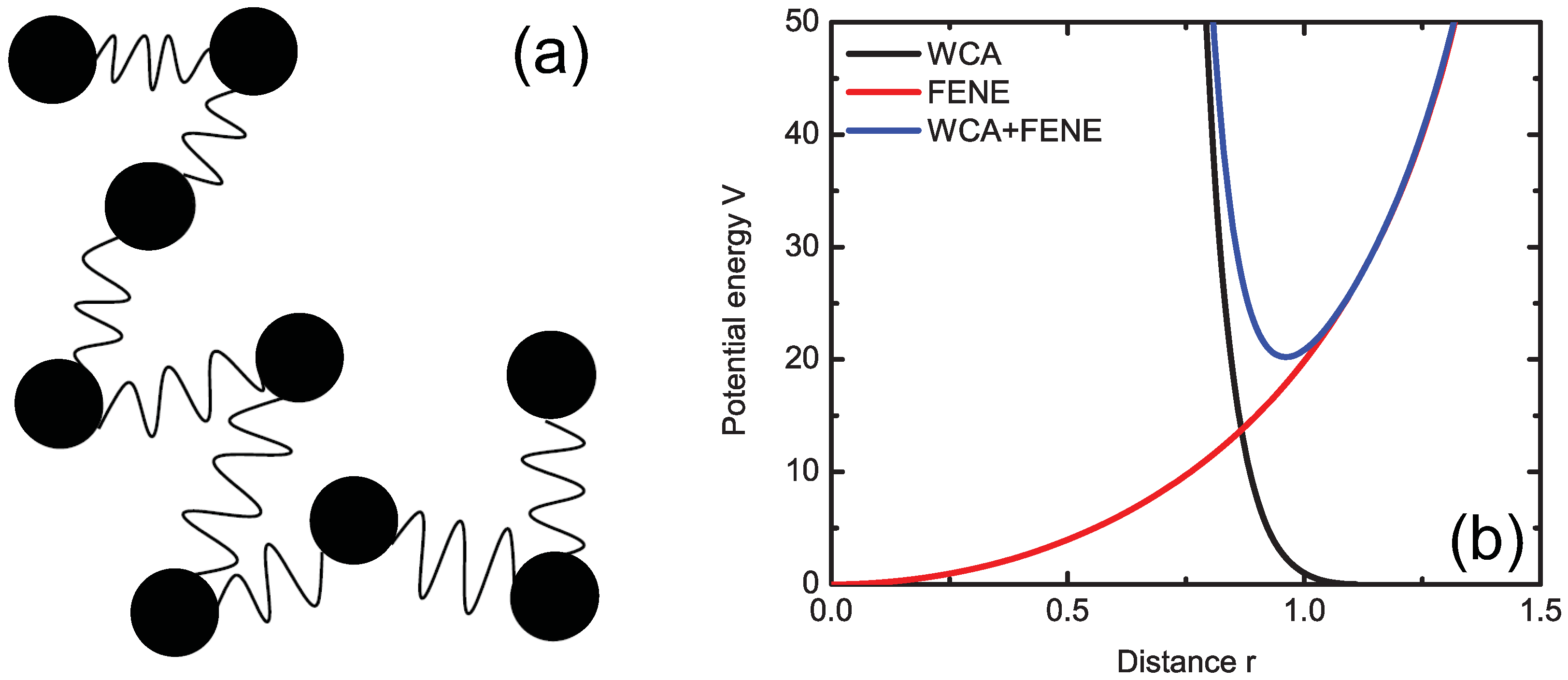
In this theoretical study on the thermodynamics of polymers, the space is divided into an equally spaced, d-dimensional, cubic lattice, and each monomer is confined to a single lattice site without any overlap, as shown in Figure 2a. The bond-fluctuation model (BFM) adopts this lattice structure, allowing the bond lengths and the angles between two consecutive bonds to vary within discrete sets of values [67,77,93]. Bonds with lengths greater than four are considered to be broken, so the bond length is restricted to be less than four [77]. Then, a monomer is randomly selected and moved onto one of its 2 d nearest-neighbor lattice sites randomly. If both the bond length restriction and the self-avoiding walk condition are satisfied, the move will be accepted. Otherwise, another monomer will be selected randomly, and so on, according to the standard Monte Carlo (MC) recipe. Here, one MC step is one attempted move per monomer of the system.
Figure 2. Depiction of (a) the bond-fluctuation model and (b) mean-squared displacements for a self-avoiding walk with N = 200 steps. Part (b) reproduced with permission from [94].
Polymers 05 00751 g002
The BFM model is very simple and efficient for modeling the dynamic properties of unentangled and entangled polymer chains. Paul et al. [94,95] applied the BFM model to study the dynamic behavior of self-avoiding polymer chains on a cubic lattice ( d = 3 ). The mean-squared displacement (MSD) of the innermost monomers, g 1 ( t ) , and the MSD of the center of mass of the entire chain, g 3 ( t ) , were calculated and plotted against the number of Monte Carlo steps per monomer, as shown in Figure 2b. According to the tube model [6], g 1 ( t ) t 0.5 and g 3 ( t ) t for the self-avoiding walk, when t < τ e . When τ e < t < τ R , g 1 ( t ) t 0.25 and g 3 ( t ) t 0.5 , while g 1 ( t ) t 0.5 and g 3 ( t ) t for τ R < t < τ d . When t > τ d , the tube constraints are completely released and g 1 ( t ) t and g 3 ( t ) t . Here, the chain length is N = 200 , which indicates that the chain is slightly entangled (entanglement length N e 30 ) [94]. As such, the MSD, g 1 ( t ) and g 3 ( t ) , exhibit similar trends, as compared with the scaling laws predicted by the tube model, but do not obey exactly these scaling exponents, as shown in Figure 2b.
Shaffer adopted the BFM to study the effect of chain topology on polymer dynamics [96]. By disallowing bond crossings, entanglements were created. From the detailed investigation of polymer chains with lengths between N = 10 and N = 300 , Shaffer found that D cm N - 2.08 and D cm N - 1 for long chains with and without entanglements, respectively. These simulations illustrate the importance of the entanglement effect on the dynamics of polymer chains. Shanbhag and Larson applied the primitive path analysis (PPA) algorithm [97] to study the primitive path of the BFM. The obtained results confirm the quadratic form for the potential of tube-diameter fluctuation, with a prefactor of 1.5, which has been theoretically predicted by Doi and Kuzuu [98]. However, the BFM is a Monte Carlo simulation and cannot be applied to study the dynamic moduli and the viscosity of polymers. The obtained results are also very generic and cannot be directly compared with numerical values for specific polymers. Subsequent works focused on the mapping of BFM results to real polymers, such as bisphenol polycarbonates and polyethylene (PE) [99,100,101,102]. The coarse-grained study of polymers using BFM has been reviewed by Baschnagel et al. [35,93].

3.2. FENE Model

One of the most widely used coarse-grained MD models for generic polymers is the finite-extensible non-linear elastic (FENE) model [16]. In the FENE model, monomers are lumped together into spherical beads, which are connected through elastic springs, as shown in Figure 3a. For dense polymeric systems, all the beads interact with each other through the Weeks-Chandler-Andersen (WCA) potential [103], which is a Lennard-Jones potential cut off at its minimum and shifted to zero. Therefore, the WCA potential is continuous and differentiable in the entire range of interaction:
V WCA r = 4 ε σ r 12 - σ r 6 + 1 4 , r < r cutoff = 2 6 σ
when r r cutoff , V WCA = 0 , as shown in Figure 3b. Here, 2 6 σ and ε represent the non-bonded diameter and interaction strength of the polymeric beads, which serve as dimensional units of simulated, dimensionless quantities. Thus, σ and ε are set to unity. Similarly, the bead mass, m, is also set to unity. r cutoff is the cutoff distance for the WCA potential. By setting Boltzmann’s constant, k B = 1 , the unit of time is given by t = σ m / ε = 1 . By taking m, σ, ε and k B as fundamental quantities, all the other units can be defined and are so-called reduced LJ units [16].
Figure 3. Depiction of (a) the FENE model and (b) its potential functions.
Polymers 05 00751 g003
The bonded beads interact, in addition, through the FENE potential [78,79]:
V FENE r = - 1 2 K R 0 2 ln 1 - r R 0 2
where K is the bond strength (usually K = 30 , to avoid bond crossing) and R 0 = 1.5 σ is used as the maximum bond length. Since the FENE potential is attractive and the WCA potential repulsive, the combination of them forms an anharmonic spring (Figure 3b). The equilibrium mean bond length is about 0.97 σ at a temperature of T = 1 . For melts, the bead number density, ρ, is fixed to be 0.85 , and the system temperature is controlled by a Langevin thermostat with a weak friction constant of 0.5 [79].
The main advantage of the FENE model is that the computationally expensive long-range van der Waals (vdW) interactions between polymeric beads, as well as the square root operation involved in calculating a harmonic bond energy are avoided. Additionally, several monomers are coarse-grained into one bead, which greatly reduces the degrees of freedom, and the Einstein frequency determining the MD time step is basically set by the WCA potential, whose thermo-mechanical properties are well known [104]. Therefore, simulation of the FENE model is extremely fast compared with all-atomistic and united-atom simulations. The united-atom method involves ignoring hydrogen atoms and is reviewed in [2,3]. Using the FENE model, Kremer and Grest [79,105] performed the pioneering works on modeling the dynamic behavior of unentangled and entangled polymer chains in equilibrium. As shown in Figure 4a, when the polymer chain length, N, is shorter than the entanglement length, N e , the dynamics of the polymer chain follows the Rouse model, as D D Rouse [1]. Here, D Rouse is the diffusion coefficient of polymer chains predicted by the Rouse model. However, if the chain length, N, is longer than N e , the dynamics of the chains will be constrained by the entanglements, such that D N - 1 D Rouse , as predicted by the tube model [6]. These obtained scaling relationships also agree exceptionally well with experimental observations, given in Figure 4a. Via non-equilibrium molecular dynamics (NEMD), Kröger and Hess [106] applied the same model to study the non-Newtonian viscosity, normal stress differences and flow-induced alignment of polymers. The zero-rate shear viscosity, η 0 , of unentangled and entangled polymer chains was also obtained. The scaling law between chain length, N, and η 0 was found to be in accordance with the prediction from the Rouse and tube models: η 0 N and η 0 N 3 for unentangled and entangled chains [106] (see Figure 4b), respectively. Moreover, in the intermediate range, the scaling relationship, η 0 N 3.4 , induced by the CLF and CR effects was also confirmed [106]. Pütz et al. [105] studied the dynamic scattering factor, S ( q ) , of entangled polymer chains and found that the S ( q ) of highly entangled polymer chains ( N = 10 , 000 ) can be well characterized by the tube model [5,107]. In addition, the entanglement length, N e , predicted from the S ( q ) calculation is in agreement with the N e obtained from the segment motion of polymer chains [105], which further validates the tube model for entangled polymer chain dynamics. Cifre et al. [108] studied the linear viscoelastic properties of unentangled polymers via NEMD simulations. By using the time-temperature superposition principle, the NEMD simulations have been extended to study the linear viscoelastic properties of FENE polymer over a broad range of frequency. The calculated storage, G , and loss, G , moduli of FENE polymers were found to agree reasonably well with the prediction of the Rouse model [109]. In addition, the empirical Cox-Merz rule [110] for polymer viscosity was also confirmed using NEMD simulations of FENE chains [108].
Figure 4. Results of (a) self-diffusion coefficient and (b) zero-rate shear viscosity of finite-extensible non-linear elastic (FENE) chains. In (a), the scaled diffusion coefficient, D ( N ) / D R ( N ) , is plotted against the scaled chain length, N / N e , p , for polystyrene (closed circles N e , p = 140 and T = 485 K [111]), polyethylene (closed squares N e , p = 31 and T = 448 K [112]), hydrogenated polybutadiene (closed triangles N e , p = 18 and T = 448 K [113]), FENE (open triangles N e , p = 72 [105]), bond-fluctuation model (BFM) (open squares Φ = 0.5 [94]) and tangent hard spheres (open circles Φ = 0.45 [114]). In (b), the data are reproduced with permission from [106].
Polymers 05 00751 g004
As aforementioned, the FENE chain model is very simple and efficient for large-scale simulations. It is very suitable as a generic model to explore and test the dynamic and mechanical properties of polymers. Therefore, it is one of the most widely used models to study polymeric materials. However, its disadvantage is also very obvious. The potential functions of FENE chains are oversimplified. For example, the backbone stiffness of polymer chains is not considered [115], since a bending potential, as employed for semiflexible chains [16,116,117,118], is not explicitly included. It is difficult to directly compare the obtained results with real polymer chemistry and physics, although different mapping methods between FENE chains and real polymers have been suggested [79,106].
To overcome these issues, a backbone bending potential was incorporated into the FENE model as V bend = k bend [ 1 - cos ( θ - θ 0 ) ] , where θ 0 = 180 is the equilibrium angle [116]. When increasing the bending stiffness, k bend , from 0 to 2 ε , the entanglement length, N e , was reduced from 70 to 20 [97,119], thus increasing the effective chain length. With this bending potential added into the FENE model, a scaling law between the entanglement length and the reduced polymer density was derived from computer simulation results and scaling arguments [120]. The obtained scaling law is found to be consistent with the experimental results on different polymer classes for the entire range, from loosely to tightly entangled polymers [120]. Therefore, including the bending potential into the FENE model is a very common extension [16,121,122,123]. For example, the FENE model with finite bending stiffness has been applied to study the static structure and dynamics of ring polymers [124,125,126]. Aside from including a bending potential, there have now been a number of studies of the FENE model where the cutoff has been increased to include the attractive well, i.e., r cutoff = 1.5∼2.5 σ. With the attractive well, the FENE model has been applied to study the glass transition temperature [127,128,129,130], scission and recombination in worm-like micelles and equilibrium polymers [131,132,133,134], surface tension [135], dielectric relaxation [136], polymer welding [137,138], strain hardening [121,122] and other properties.

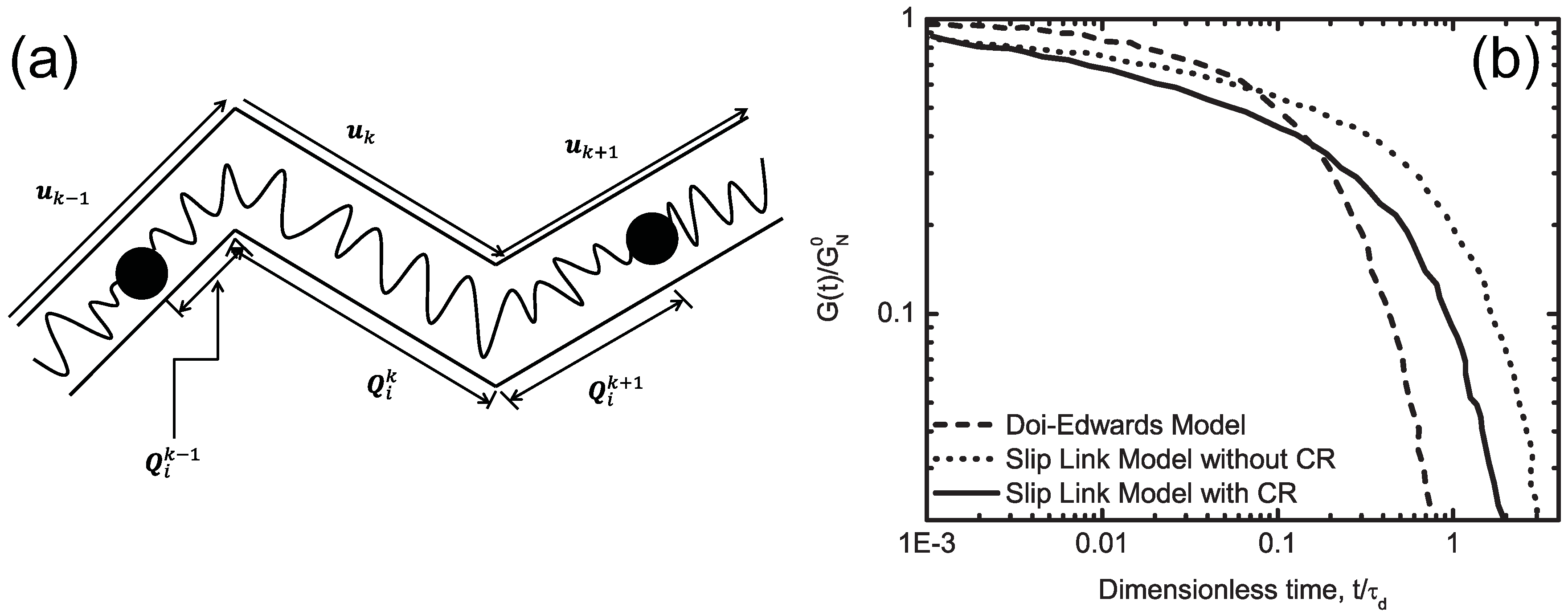
3.3. Slip-Link Model

Both the BFM and FENE model are used to simulate generic polymer chains at the level of a Kuhn step length. To further extend the spatial and temporal scales of these generic simulation methods, Hua and Schieber [33,80,81] performed the pioneering works in developing the slip-link model, based on the concept of the tube model, as illustrated in Figure 5a. In the slip-link model, the molecular details on the monomer or Kuhn-length level are smeared out, while the segmental network of generic polymers is directly modeled, which is similar to a crosslinked polymer network. However, the crosslinks in the slip-link model represent the entanglements in a polymer melt and are not permanent. They are temporary and constrain the motion of monomers of each chain into a tubular region by allowing them to slide through the slip-link constraints. The motion of segments is updated stochastically, and the positions of slip-links are either fixed in space, or mobile. When either of the constrained segments slithers out of a slip-link constraint, they are considered to be disentangled, and the slip-link is destroyed. Conversely, the end of one segment can hop towards another segment and create another new entanglement or slip-link. From the tube model [5,6], it is known that the motion of the PP makes the primary contribution to the rheological properties of entangled polymer melts. Therefore, from the microscopic information given by the slip-link model, we can precisely access the longest polymer chain relaxation time, which is quite impossible in MD simulations of dynamically entangled polymer chains. Moreover, from the ordering, spatial location and aging of the entanglements or slip-links in the simulations, the macroscopic properties of polymer melts, i.e., stress and dielectric relaxation, can be calculated through mathematical formulations [80,81].
Figure 5. Illustrations for (a) the slip-link model and (b) shear relaxation moduli G ( t ) given by different models. Figures reproduced with permission from [80].
Polymers 05 00751 g005
In contrast to the original Doi-Edwards tube model [6], the slip-link model of Hua and Schieber [80] accounts for (i) the effect of the relative velocity on the chain-tube friction; (ii) the chain stretching induced by additional chain-tube interactions; (iii) segment connectivity; (iv) chain-length fluctuation or breathing and (v) constraint release. The governing equations in the slip-link model can be separated into two parts [80]: the chain motion governed by Langevin equations and the tube motion governed by deterministic convection and stochastic constraint release processes. The motion of a chain is confined by its tube, which is assumed to be convected affinely with the flow field. In addition, the tube can undergo a constraint-release process along its contour. As shown in Figure 5a, the chain is modeled by a bead-spring chain with N beads, confined to a tube. The chain can escape the tube from its two ends by reptation or random motion, governed by the Langevin equation. The orientation of the tube segment during the deformation can be directly obtained from the deformation gradient tensor, since it is deformed affinely with the flow. However, we should emphasize that the chain inside the tube does not convect affinely with the flow, due to the friction between the chain and its tube. Thus, the equations of motion for both the chain and its tube have to be solved simultaneously in the slip-link model. There are five fundamental parameters in this model: the friction coefficient, ζ, the number of beads per chain, N, the Kuhn step length, b, the number of Kuhn steps, N K , and the tube diameter, a pp . Here, N K and b are known for a specific polymer from the polymer chemistry. ζ and a pp can be obtained through the average number of entanglements per chain, Z eq , and disentanglement time, τ d . The shear relaxation moduli, G ( t ) , simulated with different models are shown in Figure 5b. It is clear that the G ( t ) given by the Doi-Edwards model decays very quickly, compared with the slip-link model, since the Doi-Edwards model only considers reptation, whereas the slip-link model contains other relaxation mechanisms, i.e., the chain fluctuation and constraint release. When comparing the results of the slip-link model with and without constraint release, the stress relaxation is enhanced with its inclusion; the zero-rate shear viscosity, η 0 = G t d t , is reduced by a factor of 3 / 5 when constraint release is included [80].
Since the first slip slink model was introduced by Hua and Schieber [80], several related models have been developed with different resolutions and algorithmic details. Shanbhag et al. [139] developed a dual slip-link model with chain-end fluctuations for entangled star polymers, which explained the observed deviations from the “dynamic dilution” equation in the dielectric and stress relaxation data. Doi and Takimoto [140] adopted the dual slip-link model to study the nonlinear rheology of linear and star polymers with arbitrary molecular weight distribution. The strain-hardening behavior of polymer blends has been observed with 5% highly entangled chains [140]. Likhtman [141] introduced a new single-chain dynamic slip-link model to describe the experimental results for neutron spin echo, linear rheology and diffusion of monodisperse polymer melts. All the parameters in this model were obtained from one experiment and were applied to predict other experimental results. Schieber and his co-workers studied the fluctuation effect on the chain’s entanglement and viscosity using a mean-field model [142,143]. Masubuchi et al. [144] proposed a primitive chain network (PCN) model from the concept of the slip-link model. In the PCN model, the polymer chain is coarse-grained into segments connected by entanglements. Different segments are coupled together through the force balance at the entanglement node. The Langevin equation is applied to update the positions of these entanglement nodes, by incorporating the tension force from chain segments and an osmotic force caused by density fluctuations. The entanglement nodes are modeled as slip-links. The creation and annihilation of entanglements are controlled by the number of monomers at chain ends. The longest relaxation time was found to scale with the number of entanglements, Z, as Z 3.5 ± 0.1 , while the self-diffusion coefficient was found to scale as D cm Z - 2.4 ± 0.2 ; both agree well with experimental results [144]. Later on, the PCN model was extended to study the relationship between entanglement length and plateau modulus [145,146,147,148,149]. It was also extended to study star and branched polymers [150], nonlinear rheology [151,152,153], phase separation in polymer blends [154,155], block copolymers [156] and the dynamics of confined polymers [157]. Chappa et al. [158] proposed a translationally invariant slip-link model for the dynamics of entangled polymers. The proposed model can correctly describe many aspects of the dynamic and rheological properties of entangled polymer melts, i.e., segmental mean-squared displacement, shear thinning and reduction of entanglements under shear flow [158]. In addition, Ramírez-Hernández et al. presented a more general formalism based on the slip-link model to quantitatively capture the linear rheology of pure homopolymers and their blends, as well as the nonlinear rheology of highly entangled polymers and the dynamics of diblock copolymers [159]. However, so far, there is no direct mapping from the BFM or FENE model to the slip-link model, which could identify the explicit spatial locations of entanglement nodes modeled by slip-links. Such a mapping scheme could help to discriminate between the proposed slip-link models.

4. Systematic Coarse-Graining Methods

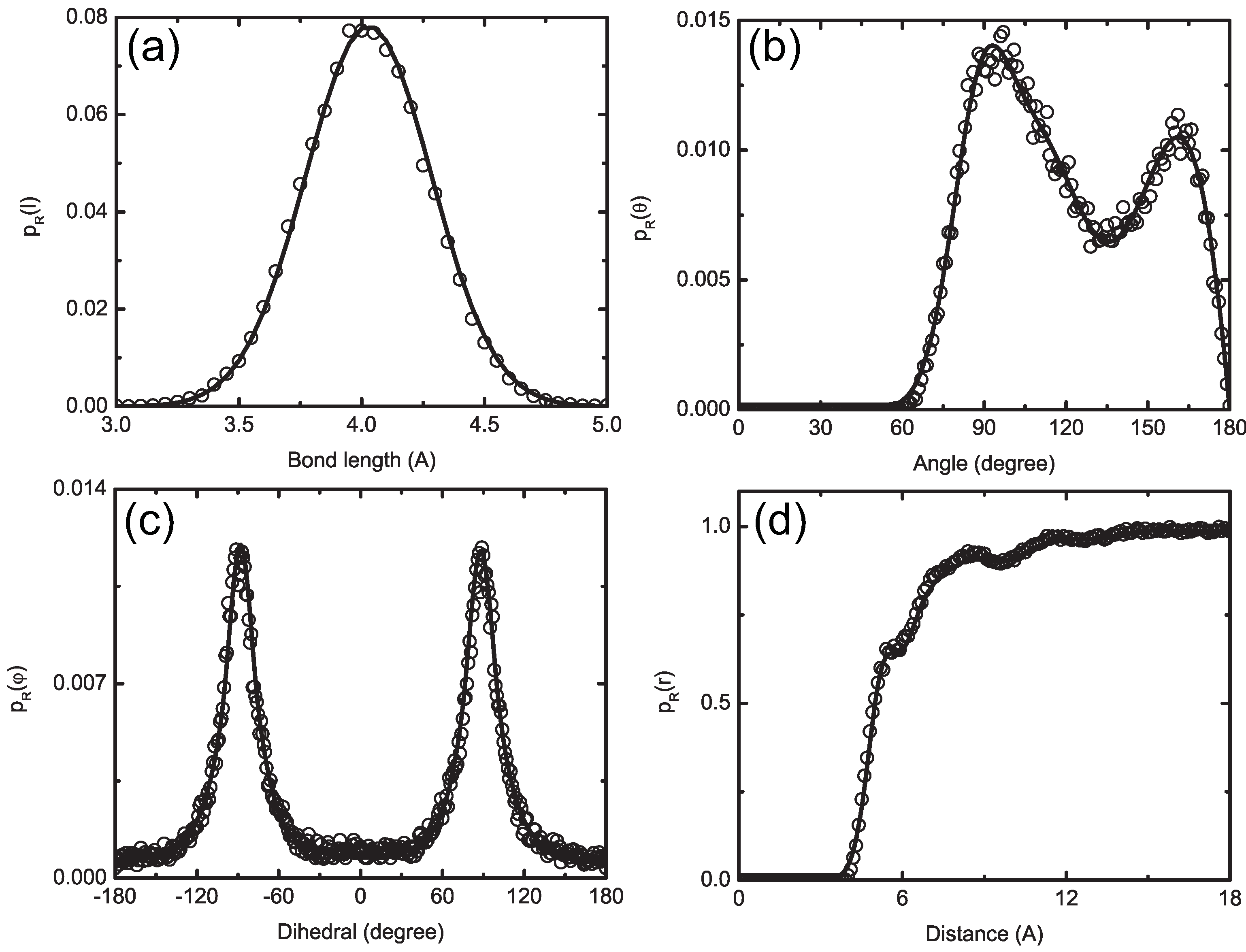
4.1. Iterative Boltzmann Inversion Method

According to their different purposes, the systematic coarse-graining methods (i.e., those with low degrees of coarse graining) can be divided into two different methodological approaches: parameterized and derived coarse-graining methods. In the parameterized coarse-graining methods, the all-atomistic simulations are used to calculate target properties, i.e., pair distribution function or force distribution, and the coarse-graining potentials are constructed to reproduce these target quantities. However, they cannot be guaranteed to reproduce all the properties of the original system, as discussed below. The derived coarse-graining methods employ direct all-atomistic simulations between the defined super atoms to derive the corresponding coarse-grained interactions. The derived potentials are not optimized to reproduce the target quantities; these quantities are, instead, predicted by the derived coarse-grained model. These derived potentials have clear physical meanings, representing the potential of mean force between super atoms. Therefore, they also have good transferability and can be systematically modified to include multibody effects, such as the effect of solvent in implicit-solvent models [160,161]. There are three methods belonging to the derived coarse-graining methods: pair potential of mean force [160], effective force coarse-graining [162] and conditional reversible work [163]. For a comparison between these methods, we refer to [43].
In the parameterized coarse-graining methods, there are structure- and force-based methods, depending on the target quantities. If the method aims to reproduce the target pair distribution functions given by the all-atomistic simulations, then it is structure-based. The structure-based methods include the iterative Boltzmann inversion (IBI) method [82,83], the Kirkwood-Buff IBI method [164], the inverse Monte Carlo (IMC) method [165], the relative entropy method [166] and the generalized Yvon–Born–Green theory [167]. All structure-based methods follow the IBI method in spirit, but with different optimization or mapping schemes. The force-based methods aim to match the force distribution on a super atom within the coarse-grained model to that obtained from all-atomistic simulation. There are two methods belonging to the force-based methods: the force-matching method [168] and the multiscale coarse-graining method [169,170]. The latter was validated through rigorous statistical thermodynamic formulations by Noid et al. [171,172,173]. Rühle et al. [174] implemented the IBI, IMC and force-matching methods into a toolkit and compared them by coarse-graining water molecules, liquid methanol, liquid propane and a single molecule of hexane. They found that each method had its own advantages and disadvantages. Readers interested in more details of the related methods mentioned may wish to inspect the referenced materials. Of the methods mentioned, the IBI method is one of most widely used and is discussed in detail below.
As shown in Figure 6, the all-atomistic model contains n atoms with Cartesian coordinates, r n = r 1 , , r n . These n atoms interact with each other through the inter-atomic potential, u ( r n ) . According to the canonical equilibrium distribution function [175], the configurational probability distribution of atomic positions, r n , for the all-atomistic model at given volume, V, and temperature, T, is [82,83]:
p r ( r n ) = 1 z n e - u ( r n ) / k B T
where z n = z n , V , T = d r n e - u ( r n ) / k B T is the partition function, an integral over all the possible atomic coordinates. By grouping a small number of atoms into one single interaction site, given in Figure 6, the all-atomistic model can be mapped into a coarse-grained model with N super atoms. The coordinates of the N super atoms in the coarse-grained model are represented by R N . The corresponding mapping matrix M RI between r n and R N is defined as R N = M RI r n . Analogous to the all-atomistic representation, the probability distribution of positions for these super atoms at the given V and T is obtained as the following:
P R ( R N ) = 1 Z N e - U ( R N ) / k B T
where Z N = Z N , V , T = d R N e - U ( R N ) / k B T is the partition function for the coarse-grained system. The U ( R N ) is the inter-atomic potential function for the super atoms. In order for the all-atomistic model to be consistent with its corresponding coarse-grained model, the two probability distribution functions should satisfy the following condition:
P R ( R N ) = p R ( R N )
Here, p R ( R N ) = d r n p r ( r n ) δ ( R N - M RI r n ) . Consequently, a rigorous connection between the potential functions, u r n and U R N , is defined through an ab initio coarse-graining procedure:
e - U ( R N ) k B T = Z N z n d r n e - u ( r n ) / k B T δ R N - M RI r n
From the above equation, it is clear that the derived coarse-grained potential function, U ( R N ) , is not a conventional potential energy function [82,83,176,177]. The potential function, U ( R N ) , contains many-body effects and highly depends on the configurational free energy function or potential of mean force (PMF) of the thermodynamic state point. Thus, U ( R N ) relies both on energetic and entropic effects, which should affect the dynamic behavior of the coarse-grained model. Such an effect will be explained below.
Figure 6. Illustration for mapping from the all-atomistic model ( r n ) to the coarse-grained model ( R N ), with a mapping operator, M RI , using the polymer cis-polyisoprene.
Polymers 05 00751 g006
In practice, the probability distribution function for the all-atomistic model, p r ( r n ) , can be estimated directly from trajectories of Monte Carlo or MD simulations. To be specific, the potential function for the corresponding coarse-grained system is determined through the following equation [82,176]:
U ( R N ) = - k B T ln p R ( R N )
That is, according to the relationship between p r ( r n ) and p R ( R N ) , the potential function, U ( R N ) , can be numerically determined. In most cases, the probability distribution function, p R , is considered to depend on the following four variables: pair distance, r, bond length, l, bond angle, θ, and dihedral angle, ψ, as p R ( R N ) = p R r , l , θ , ψ . If we assume that these four variables are independent of each other, then p R r , l , θ , ψ = p R r p R l p R θ p R ψ , and the potential function for the coarse-grained model becomes U ( R N ) = U ( r , l , θ , ψ ) = U ( r ) + U ( l ) + U ( θ ) + U ( ψ ) ; i.e., U ( q ) = - k B T ln p R q with q = r , l , θ , ψ for pair, bond, angle and dihedral interactions, respectively. In the interest of reproducing the distribution function of the all-atomistic model as accurately as possible via the coarse-grained model, additional iterations of this numerical process are often undertaken [92,178]:
U n + 1 q = U n q + Δ U n q
Δ U n q = k B T ln p R n q p R target q
where p R target are the target distribution functions calculated from the all-atomistic simulations. Thus, the distribution functions, p R , can converge to the target distribution functions, p R target , after several iterations.
The typical procedure for the IBI is illustrated in Figure 7. The target distributions, p R target , are obtained from all-atomistic simulations after defining the super atoms for the coarse-grained model, which is not shown in this workflow. The “Global initialization” module organizes all the paths for the input files, executables, etc. Next, the “Iteration initialization” module converts the target distribution functions, p R target , into the internal format and smooths them. Subsequently, the smoothed target functions are used to calculate the initial guesses for the potential functions of the coarse-grained model in the “Prepare sampling” module. With the input files from the “Iteration initialization” module and the potential files from the “Prepare sampling” module, the “Sampling” module will run the canonical MD or Monte Carlo simulations to generate the trajectories of the coarse-grained model. From these trajectories, the distribution functions, p R n , are calculated, as well as the potential updates, Δ U n , in the “Calculate updates” module. After this, the potential updates, Δ U n , are smoothed and extrapolated in the “Post-processing of updates” module. The updated potential functions, U n + 1 , are calculated via U n + 1 = U n + Δ U n in the “Update potentials” module. The updated potential functions, U n + 1 , are further smoothed and extrapolated in the “Post-processing of potentials” module. The convergence of the potential updates, Δ U n , or distribution functions, p R , will be further evaluated. If a convergence criterion is met, the iteration process is stopped and the obtained potential function returned. Otherwise, the algorithm proceeds with the next iteration step to optimize the potential functions. Within this process, the “Sampling” and “Calculate updates” are obviously the most time-consuming modules.
Figure 7. Workflow chart for the Iterative Boltzmann Inversion (IBI) method. The figure is taken and modified from [174].
Polymers 05 00751 g007
Here, we use cis-polyisoprene (PI) polymer, which is one of the most widely used polymers, as an example to demonstrate the IBI method. As shown in Figure 6, there are five carbon atoms per monomer. Four of them are connected sequentially to form the backbone. The fifth one is connected to the backbone as a side chain. The center of the monomer lies on the center of the carbon-carbon double bond, and the PI polymer chain is formed by all head-to-tail linkages between monomers. The all-atomistic model for PI was defined by 100 chains with 10 monomers per chain, which was built using the Amorphous Cell module in the Materials Studio software package [179]. The side length of the simulation box was around 54 Å, with periodic boundary conditions. The ab initio force field COMPASS [180] was used for the all-atomistic simulations. The MD simulation was performed under the N V T ensemble with a temperature of T = 413 K and a time step of t = 1 fs. Twenty snapshots of the trajectory were taken over a 10 ns simulation. The Amorphous Cell module may generate unphysical initial structures for polymers, but investigation of the rheological properties of polymers requires proper equilibration. Therefore, we compared our equilibrated all-atomistic cis-PI polymer structure with that reported by other researchers [181], through the radius of gyration, end-to-end distance and the pair distribution function between different monomers. All these quantities are found to be in accordance with the published results [181], and we therefore consider the cis-PI polymer used in our work to be well equilibrated. As shown in Figure 6, the center of the super atom in the coarse-grained model was defined as the center of the carbon-carbon bond connecting two monomers, instead of the center of the PI monomer (to be discussed in the following section). With the super atom thus defined, the super-atomic coordinates can be directly mapped from the all-atomistic model. The distribution functions, p R ( q ) , obtained from the all-atomistic simulation trajectories, are shown in Figure 8.
Once the target distribution functions, p R target , were obtained from all-atomistic simulations, the initial-guess potential functions for the corresponding coarse-grained model were calculated as U 0 ( l ) = - k B T ln p R target ( l ) , U 0 ( θ ) = - k B T ln p R target ( θ ) / sin ( θ ) , U 0 ( ψ ) = - k B T ln p R target ( ψ ) and U 0 ( r ) = - k B T ln p R target ( r ) . The appearance of sin ( θ ) in U 0 ( θ ) is a result of the mathematical derivation of the IBI method and is explained in [82,83,176,177]. These initial-guess potentials were used in canonical coarse-grained MD simulations and, then, iteratively optimized according to Equation (8). After 15 iterations, the obtained distribution functions from the coarse-grained MD simulations were found to be in agreement with the target distribution functions, as shown in Figure 8. The final potential functions for the coarse-grained model for PI obtained after completion of the iteration process are shown in Figure 9. Here, we found that 15 iterations of the IBI method were sufficient to yield good results for our PI polymer, due to the correct definition of super atom and the initial potentials used. In general, the number of iterations required within the IBI method depends on polymer structure, the definition of super atom, degree of coarse-graining, initial potentials, etc., and hundreds of iterations may be required to reach convergence [174]. It should be noted, as shown in Figure 9d, that the pair interaction is purely repulsive, due to the lack of correlation “spikes” in p R target ( r ) , as shown in Figure 8d. This is a common problem with systematically coarse-grained potentials, and it induces anomalous pressures in simulations. To obtain the correct pressure for the coarse-grained model, a linear attractive function can be added to the tail of the pair potential, as discussed below. The potentials given in Figure 9 should be used only for the NVT ensemble that operates at the correct density of the PI polymer.
Figure 8. Distribution functions for (a) bond length; (b) bond angle; (c) dihedral angle; and (d) pair distance of all atomistic (solid lines) and coarse-grained (dots) models of cis-polyisoprene (PI) melts at 413 K. Figure reproduced with permission from [92].
Polymers 05 00751 g008
Figure 9. Optimized potential functions for (a) bond; (b) angle; (c) dihedral and (d) pair interactions of coarse-grained cis-PI melts at 413 K. Figure reproduced with permission from [92].
Polymers 05 00751 g009
Although the IBI method is a very straightforward and systematic coarse-graining method with rigorous thermodynamical foundations [82,83,176,177], there are several important issues that require attention and further discussion.

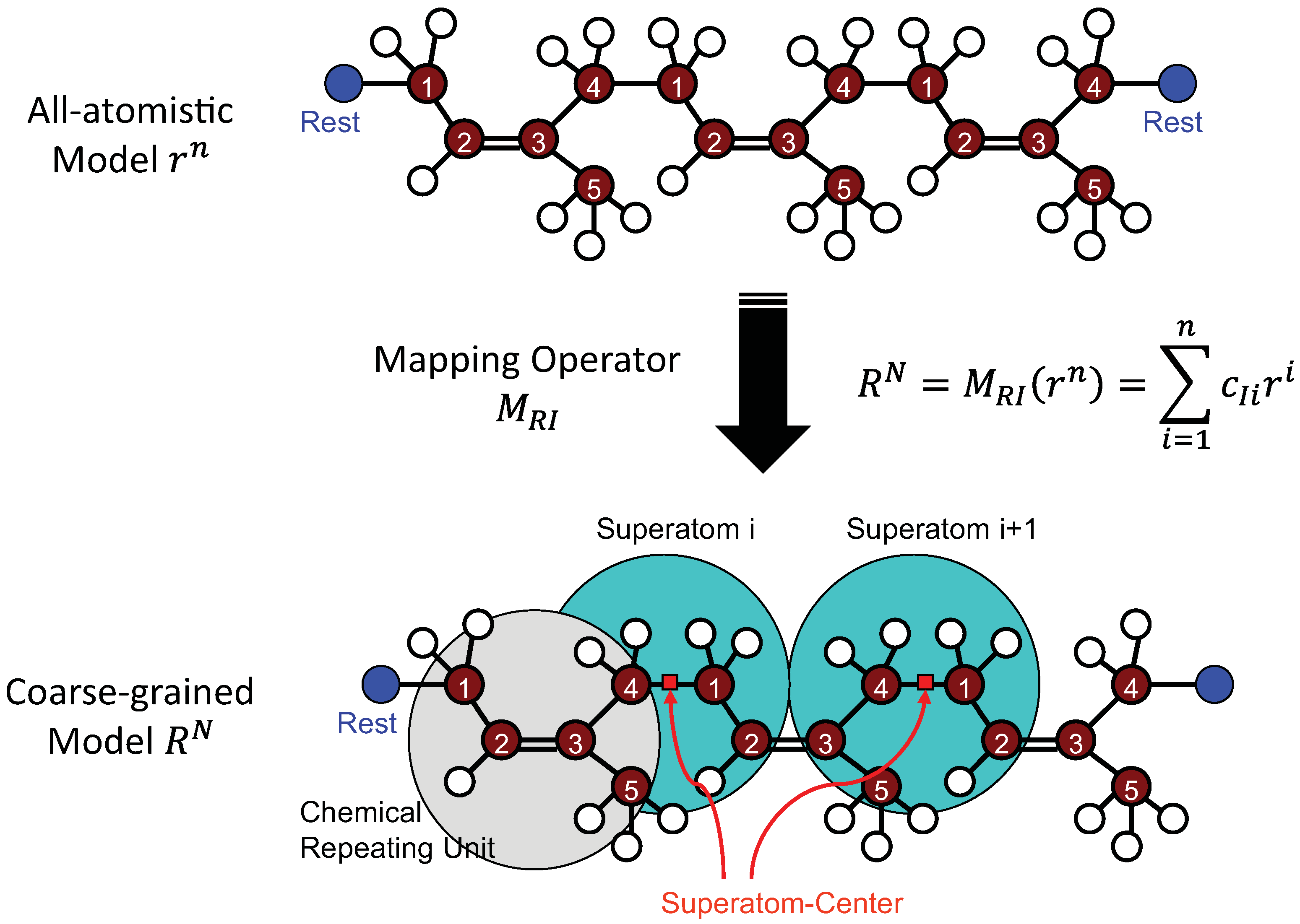
4.1.1. Definition of Super Atom

The aforementioned mapping matrix, M RI , is not unique, since there are multiple ways to define the super atoms. When different mapping matrices are used, the obtained coarse-grained potential functions are also quite different. The obvious question is, “How to define the super atom?” or alternatively, “Is there a criterion to determine whether a given super-atom definition is appropriate?” This is actually a very important question when using the IBI method. As shown in Figure 6, there are at least two ways to define the center of super atoms for cis-PI. One is the center of the PI monomer, and the other is the center of the carbon-carbon bond connecting two monomers together. The distribution functions, p R ( l ) , for both of these definitions have been obtained (Figure 10). In the first case, p R ( l ) is characterized well by a single Gaussian, and from Equation (7), the corresponding bond potential function is harmonic, where the height-to-width ratio of the Gaussian defines the strength of the harmonic bond and the equilibrium bond length is determined by the location of the peak. However, in the second case, p R ( l ) is doubly peaked (see Figure 10b). The underlying reason for these two different distributions is that the carbon-carbon double bond is very rigid in torsion, while the carbon-carbon single bonds can easily flip from one torsional state to another. Thus, if the super-atomic center is defined as the center of mass of the cis-PI monomer (i.e., the carbon-carbon double bond), the p R ( l ) will have two peaks, corresponding to the two torsional states of the carbon-carbon single bonds that effectively connect the super atoms together. Of course, this cannot be modeled by a single harmonic potential. Similar behavior is also found in cis-1-4 PI and trans-PI polymers by Faller and his co-workers [37,68,182,183,184,185,186].
Figure 10. Bond-length distribution functions for a super atom of cis-PI defined (a) at the center of a carbon-carbon single bond connecting two monomers and (b) at the center of the monomer. The inserts show the bond-length versus bond-angle distributions.
Polymers 05 00751 g010
The multiplicity of peaks for p R ( l ) can lead to interdependence of the bond-length and -angle potential functions. As shown in the insert of Figure 10a, the bonds and angles can be plotted following the idea of a Ramachandran diagram [187]. Comparing the two different super-atom definitions, p R ( l ) , with a single peak demonstrates a more uniform distribution of bond lengths, l, and angles, θ, suggesting their independence. In the case of the doubly peaked p R ( l ) , the correlation between l and θ is not uniform, indicating their interdependence (Figure 10b). Correlation uniformity is a basic criterion highlighting the proper choice of the super atom in coarse-graining, as it relates to whether the factorization assumption of the probability distributions is valid. Such a criterion has been checked in detail for different coarse-graining models, through combined p R ( θ ) versus p R ( ϕ ) distribution plots (see Figure 3 in [188]). It is also more convenient to represent a group of atoms as a spherical super atom with an isotropic potential, instead of an ellipsoidal super atom with anisotropic potential. In most studies, the super atom is defined to be a spherical particle [37,177,184,189,190,191], but there are also some studies attempting to do generalizations for anisotropic potentials [192,193]. However, the potential functions and the coarse-grained MD simulations become rather complex, and only slightly higher accuracy can be achieved. When a single spherical super atom is not good enough to characterize a group of atoms, it is more feasible to use more than one spherical super atom per monomer than a single non-spherical one. For example, to model polycarbonate polymers, Abrams and Kremer [194] utilized five spherical super atoms to represent one all-atomistic monomer.
Another interesting example is the coarse-graining of polystyrene (PS) via the IBI method, as illustrated in Figure 11, which has been extensively studied using different methods. Müller-Plathe and his co-workers [195,196,197] adopted the mapping scheme shown in Figure 11a using an IBI method with pressure correction. The developed model successfully reproduces the gyration radius and the Flory characteristic ratio of PS in melts (500 K). However, the obtained entanglement length is much smaller than the experimental value. Through slight modifications, Spyriouni et al. [198] improved the coarse-grained potential functions from previous works [196,197]. The optimized coarse-grained model can capture the correct entanglement length of PS melts [198]. The structure parameters, i.e., packing length and tube diameter, were also obtained and found to be in agreement with experiments [199]. However, the obtained isothermal compressibility is far from the experimental value, which indicates poor transferability of the developed potential to pressures different from the one used in the all-atomistic simulation. Sun and Faller systematically developed a coarse-grained model for isotactic PS melts from the unentangled to the entangled regime using the super atom definition shown in Figure 11b [185,200]. The obtained entanglement length at 450 K is found to be in agreement with experimental observations. Qian et al. [69] chose another mapping scheme (see Figure 11c). The newly obtained potentials can reproduce the isothermal compressibility and structure properties of the PS melts from 400 K to 500 K. Kremer and his co-workers used yet another mapping scheme, as shown in Figure 11d [188,201]. They split the PS monomer into two parts, and each of them was represented by one super atom, which is a so-called “2:1” coarse-grained model. The derived model can represent the PS sequence with varying tacticities and has been validated for the structural and dynamic properties of atactic PS [188,201]. These models have recently been used to distinguish the dynamics of iso-, syndio- and atactic PS polymers. Interestingly, the time scale factors are not identical for these models [42]. Moreover, the model can be applied to study both the mechanical properties of PS glasses [202,203] and the dynamic properties of PS melts [204,205]. From these studies, it is important to know that although there are different ways to define the super atom in deriving a coarse-grained model, the static, dynamic or thermodynamic properties of the coarse-grained model should be tested and validated before it is further applied [42].
Figure 11. Different definitions for the super atoms of coarse-grained polystyrene (PS): (a) [195,196,197]; (b) [185,200]; (c) [69]; and (d) [188,201].
Polymers 05 00751 g011

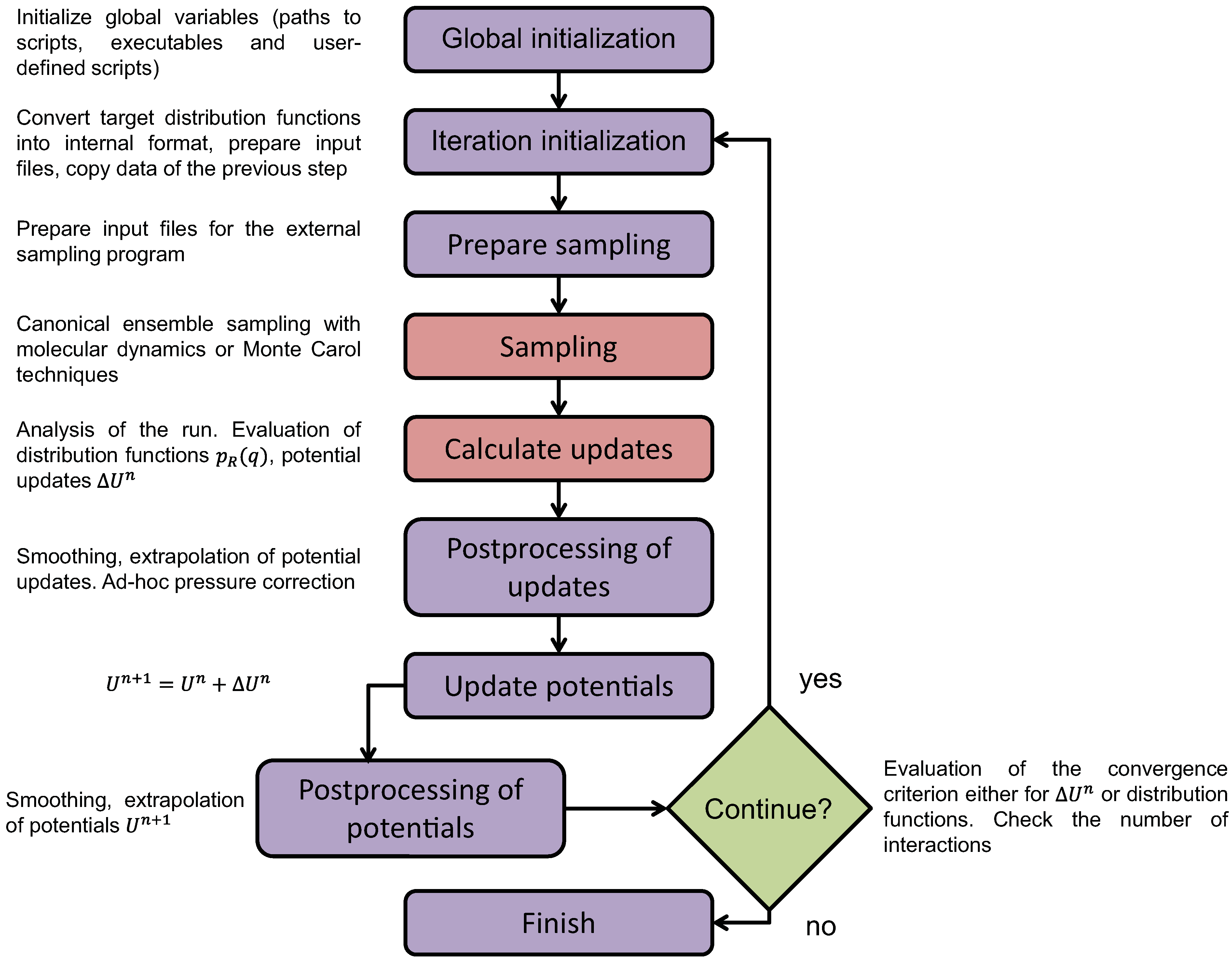
4.1.2. Smoothing, Extrapolation and Convergence

As mentioned in Figure 7, the obtained distribution and potential functions need to be smoothed and extrapolated. Moreover, some of the distribution functions, i.e., p R ( θ ) , p R ( ψ ) and p R ( r ) , shown in Figure 8 are very irregular. Thus, these distribution functions cannot be easily fitted, hindering the derivation of the effective coarse-graining potentials. Milano et al. [196] developed and discussed analytical forms for these complex distribution functions. Since these distribution functions always exhibit multiple peaks, they applied multi-centered Gaussian distribution functions to fit them [196]:
p R ( q ) = i = 1 n A i w i π / 2 e - 2 q - q c i w i 2
where q c i is the location of the ith peak, and A i and w i represent the corresponding total area and width, respectively. According to Equation (7), the potential function for each distribution is obtained via:
U ( q ) = - k B T ln i = 1 n A i w i π / 2 e - 2 q - q c i w i 2
The corresponding force is easily obtained analytically as F ( q ) = - d U ( q ) / d q . The advantage of such an analytical multi-centered Gaussian distribution function is obvious: they are continuous and differentiable at any order. Therefore, during the iteration process, the potential functions for the coarse-grained model converge rather quickly. Moreover, the fitted and extrapolated distributions are non-zero everywhere. Thus, the corresponding energy also always has finite value, which avoids any energy singularity in the simulation. In addition, such a distribution function is easily implemented into the existing software. Müller-Plathe and his collaborators developed the “It is Boltzmann Inversion software for Coarse Graining Simulations” (IBIsCO) code to incorporate this form into their coarse-grained MD simulations [206,207]. It is also possible to use the tabulated form for these complex potential functions. Luo and Sommer [208] developed a tabulated angle potential function with cubic spline interpolation to smooth both potential and force in simulations. To date, there is support for tabulated forms for all the potential functions, including pair, bond, angle and dihedral interactions, in the Large-scale Atomic/Molecular Massively Parallel Simulator (LAMMPS) [209]. Since the system pressure and density are very sensitive to the vdW interaction, the smoothness and extrapolation of the pair or vdW interaction are also important. Müller-Plathe and his co-workers adopted the automatic simplex optimization to fit this potential function [83,210,211,212]. They furthermore developed different analytical functions to fit p R ( r ) , as well [83,211].
During the smoothing and iteration process of the IBI method, the rate of convergence is of utmost practical relevance, especially for multi-component systems [174]. For one-component systems, the coarse-grained potentials easily converge, as there is only one target distribution function. However, for a two-component system, for example, consisting of components, S a and S b , there are three target radial distribution functions, ( g a a ( r ) , g b b ( r ) , and g a b ( r ) ), and three corresponding effective pair potentials ( W a a ( r ) , W b b ( r ) and W a b ( r ) ), which are correlated with each other. However, in the IBI method, the updates for g a a ( r ) , g b b ( r ) , g a b ( r ) do not account for such cross-correlations. The convergence of the IBI method is therefore not easily satisfied for multi-component systems. To overcome this issue, Lyubartsev and Laaksonen [165] developed the IMC method, in which the correlation between different distribution functions is accounted for during the updating and iterating process, and the effective potentials of the multi-component system rather quickly converge. The convergence rate can be further improved using a smoothing technique on the potential update, Δ U . Here, we should emphasize that the smoothing should not be applied to the potential, U, itself, since it has important structural features that can be destroyed if smoothing is applied haphazardly. Using a multiplicative prefactor for the update function of the pair potential, Reith et al. [212] further improved the convergence of the pair potential in the IBI method. Murtola et al. [213] adopted thermodynamic constraints in the IMC method to improve the convergence. Recently, Wang et al. [214,215] adopted a single-step coarse-grained potential scheme for poly(ethylene terephthalate) (PET), by invoking the Ornstein-Zernike equation with the Percus-Yevick approximation [214], sidestepping iteration and convergence issues. The obtained coarse-grained potentials can satisfactorily reproduce the structural and dynamic properties of PET obtained via atomistic MD simulations [215].

4.1.3. Dynamic Rescaling

In the IBI method, a group of atoms is lumped together into a spherical super atom. Thus, the internal degrees of freedom inside the super atom have been averaged out, which can change the entropy and, thus, the free-energy landscape of the system, altering the its internal dynamics after coarse-graining. In addition, since a cluster of atoms is simplified into a spherical super atom, it can also change the amount of surface of each molecule that is available to surrounding molecules. Consider an all-atomistic polymer chain immersed in water, and let the total surface available to the solvent be denoted by S solvent all . If we switch from the all-atomistic polymer chain to a bead-spring chain, whose beads are represented by spherical particles, the solvent-accessible surface of the bead-spring chain is S solvent CG . Obviously, S solvent CG S solvent all , since the surface roughness of the monomer has been smeared out in the bead-spring chain. As such, the hydrodynamic radius, r hydr , of the coarse-grained super atom in each situation is also different. According to Stokes’s law [216], the friction coefficient, ζ, is related to the hydrodynamic radius, r hydr , through the solvent viscosity, η solvent , as ζ = 6 π η solvent r hydr . Thus, in the coarse-graining process, the internal friction coefficient between monomers is typically also changed, leading to incorrect dynamic behavior of the coarse-grained system [37,217,218]. It is therefore necessary to perform dynamic mapping (i.e., rescale the dynamics) in order to simulate the correct behavior.
Faller [37] proposed several methods to perform dynamic mapping: by chain diffusion, through the segmental correlation times in the Rouse model and by direct mapping of the Lennard-Jones time. However, none of these methods can recover exactly the same dynamics of all-atomistic simulations. Harmandaris and Kremer [204,205,219,220] used short-chain atomistic and coarse-grained simulation to calculate a time-mapping constant based on the friction coefficients. In their approach, they assumed that the softer coarse-grained potential induces a reduced friction coefficient, ζ CG , between the super atoms. If we denote the friction coefficient for the realizations of these super atoms in the all-atomistic simulation as ζ AA , the corresponding time-mapping factor is determined as S AA - CG = ζ AA / ζ CG [204], in accord with the Rouse model. However, it is quite difficult to determine analytical expressions for the friction coefficients. Alternatively, one can calculate S AA - CG numerically, using the mean-squared displacement (MSD) of the monomers as the time-scaling metric, since the MSD is inversely proportional to the friction coefficient for unentangled polymer chains. As such, S AA - CG can be estimated as MSD CG / MSD AA . Although such a dynamic rescaling method does not have rigorous theoretical foundations, it has been used successfully for low degrees of coarse graining [92,183,184,197,200,201,221,222,223,224,225,226,227]. Using this mapping method, Harmandaris and Kremer [204,205] successfully mapped the dynamic behavior of PS melts from the all-atomistic scale to the coarse-grained level, as shown in Figure 12a,b. The obtained diffusion coefficients for unentangled and entangled PS melts were in agreement with the experimental results [204]. Recently, Li et al. [92] adopted the same method to map the dynamic behavior of cis-PI melts (Figure 12c,d), with a mapping ratio of S AA - CG = 11.47 . After rescaling the time of the coarse-grained simulation by this mapping ratio, both translational (MSD) and rotational (autocorrelation function of end-to-end unit vector) dynamics of cis-PI melts were correctly captured (see Figure 12c,d). Moreover, the diffusion coefficient of the highly entangled cis-PI was also directly predicted from the coarse-grained simulation without any adjustable parameters [92]. Note that in the coarse-grained PS melts, one PS monomer is coarse-grained into two super atoms, as shown in Figure 10d, and in the coarse-grained model of cis-PI, each of the PI monomers is mapped to a single super atom (see Figure 6). This small degree of coarse-graining should only produce a minor change in system entropy (compared with the change of interacting surfaces), so it is ignored in the time mapping. However, entropy change plays a much more important role in highly coarse-grained models. Finally, we would like to emphasize that time-scaling is one of the central challenges in the coarse-graining process [75,228]. It is known that different modes of motions in a system can have different time-scaling factors compared to the underlying all-atomistic model; this phenomenon is referred to as “dynamical heterogeneity” [75,228,229]. Dynamical heterogeneity is a significant problem in studying the structure formation of polymer mixtures.
Figure 12. (a) Autocorrelation function of end-to-end unit vector, R ( t ) · R ( 0 ) , and (b) mean-squared displacement g 3 ( t ) versus time for both united-atom (dots) and coarse-grained (lines) PS melts at 463 K; (c) R ( t ) · R ( 0 ) and (d) mean-squared displacement, g 1 ( t ) , versus time for both all-atomistic and coarse-grained cis-PI melts at 413 K. The time of the coarse-grained simulation has been rescaled by a factor of 11.47 in (c) and (d). Figures reproduced with permission from [92,204].
Polymers 05 00751 g012

4.1.4. Transferability and Thermodynamic Consistency

In the IBI method, the distribution functions are obtained for a specific ensemble (fixed number, N, of particles, temperature, T, and volume, V, or pressure, p). The effective potential functions are optimized against the target distribution functions, which are calculated from one set of thermodynamic conditions. The effective potential functions, however, depend on the free energy of the system, which is also state-dependent. Thus, the potential functions derived from one thermodynamic state are not usually transferable to another set of conditions (N, T and V or p), as discussed by Luis [230]. Therefore, usually, the effective potential functions will require a process of optimization for each thermodynamic state of the coarse-grained system. Naive use of interaction potentials at the coarse-grained level developed from the IBI method can lead to incorrect values for the thermodynamic properties of polymers. This is because the main goal of the IBI method is to correctly reproduce the static structure of the polymer chains by means of a set of equivalent potentials of mean forces, and as such, the effective potentials obtained from the IBI method are only approximate, and many-body effects are ignored beyond a certain number of super atoms.
However, there are several studies demonstrating that the effective potential functions of the coarse-grained model have a limited range of transferability into a subset of thermodynamics states [69,188,201,231,232,233,234,235,236]. Doi and his co-workers studied the mean densities and segment distribution functions of coarse-grained and united atom models for linear PE from 300–800 K and found that they agree well at all temperatures, except 300 K [231]. Thus, they concluded that the derived potential functions could be applied to the PE melts over a broad temperature range. Müller-Plathe and his co-workers [232] studied the transferability of the coarse-grained force fields derived with the IBI method for PS and polyamide-6,6 (PA66) polymers, systematically testing the temperature and pressure effects on the static, dynamic and thermodynamic properties by comparing the coarse-grained results with the all-atomistic ones. They found that the coarse-grained PS model (with the center of the super atoms defined on the methylene group, as shown in Figure 10b) was only transferable over a very narrow temperature range, and its bulk density change cannot be correctly predicted by the coarse-grained model when the temperature is about 80 K below the optimization temperature (500 K) [232]. In addition, the isothermal compressibility of the PS melts was also overestimated by the coarse-grained model. However, for the PA66 polymers, the derived coarse-grained model is fully transferable for different temperature and pressure states. All the intra- and inter-structural rearrangements induced by the temperature change can be correctly reproduced by the coarse-grained model [232]. Moreover, the isothermal compressibility of PA66 polymers calculated from the coarse-grained simulations at different temperatures is in accordance with the experimental values [232]. They also found that chain length did not affect the transferability of the derived potentials, and that the transferability of the PA66 coarse-grained potential was due to the lower degree of coarse graining, compared with the PS model [232]. Later, Müller-Plathe and his co-workers studied the temperature transferability of the coarse-grained potentials for ethylbenzene (EB), PS and their mixtures [69]. The center of the super atoms for PS and EB were defined to coincide with the centers of mass for each monomer, as shown in Figure 11c. The thermal expansion coefficients for PS and EB polymers were reproduced well by their coarse-grained simulations, compared with the all-atomistic simulations. It was also found that the derived coarse-grained potentials for PS melts were transferable within the temperature range 400–500 K [69]. However, the coarse-grained potential for EB is temperature-dependent, with a temperature shift factor, T / T 0 , such that U ( T ) = U 0 ( T 0 ) T / T 0 [69]. The coarse-grained potential for the EB polymer was derived at a temperature of T 0 = 298 K . The coarse-grained model for PS melts developed by Harmandaris et al. [219], with super atoms defined in Figure 10d, can capture the correct temperature and pressure dependence of PS dynamics. From the above discussion, we can see that the transferability of the coarse-grained potentials derived by the IBI method can be highly dependent on the definition of super atoms, and special attention should be paid to this choice. For homopolymer melts, for example, polyethylene [237], polybutadiene [226,238] and other polymers, the coarse-grained potentials show a remarkable transferability over a large range of temperatures.
In addition to the transferability of the coarse-grained potentials, the thermodynamic consistency of the model should also be considered. For example, in the long range, the super atoms are homogeneously arranged in space, such that p R ( r ) = 1 for r 15 Å, as shown in Figure 8d. Thus, the corresponding pair potential will be zero. However, in reality, the long-range interactions between these super atoms should be attractive, which leads to U ( r ) > 0 . Due to the missing long-range attraction, the pressure in the coarse-grained model can be overestimated [83,174,211,212]. To recover the correct pressure for the coarse-grained model, a linear, attractive tail function is usually added into the pair potential:
Δ U pressure ( r ) = A ( 1 - r / r cut )
where r cut is the cutoff distance for the pair potential and A is a fitting parameter to be used for pressure correction. The above equation also implies that Δ U pressure ( 0 ) = A and Δ U pressure ( r cut ) = 0 . This correction term mostly manifests itself when r > 1 nm. Thus, the short range pair distribution of the super atoms will not be greatly affected. Such a linear, attractive tail function has been demonstrated to recover the correct pressure for coarse-grained polymer systems [83,211,212,239,240].

4.2. Blob Model and Uncrossability of Coarse-Grained Chains

As we have mentioned for the IBI method, the definition of super atoms is not unique. Therefore, it is possible to define the super atom to represent several monomers of the polymer chain in order to extend the available length and time scale of the coarse-grained simulation. Here, the super atom is considered to be a spherical blob of radius R blob , which represents the center of mass for χ consecutive monomers. This is the basis of the so-called “blob model” [84,85,241], illustrated in Figure 13a. All the potential functions for the blob model are derived systematically from all-atomistic simulation, as in the IBI method. The blob must be spherical, so χ cannot be arbitrarily large. Otherwise, the size of the blob will exceed the tube diameter of the polymer chain. However, in order to approach the long-time relaxation behavior of the polymer chain, χ should be large enough to allow a large integration time step in simulation.
In modeling of polyethylene (PE) polymers, Padding and Briels chose χ to be 20 [84], which is about 1 / 3 of the entanglement length of PE [242]. By following the same principle of the IBI method, the potential functions for the blob model were systematically derived from the all-atomistic simulation [243]. Since the blob represents about 20 monomers of PE, the dihedral interactions between these monomers are very weak and, thus, ignored in simulation. As such, the potential functions for the blob model usually consist of non-bonded (vdW) interaction and bonded (bond and angle) interactions. According to Padding and Briels, the non-bonded interaction consists of a single repulsive Gaussian function [84]:
U r = c 0 e - r / b 0 2
where c 0 and b 0 are fitted parameters. The bond potential consists of a repulsive term described by two Gaussians and an attractive term described by a single power law [84]:
U ( l ) = U rep l + U att ( l ) = c 1 e - l / b 1 2 + c 2 e - l / b 2 2 + c 3 l μ
where c 1 , c 2 , c 3 , b 1 , b 2 and μ are fitting parameters. The angle (or bending) potential is characterized by a cosine function [84]:
U ( θ ) = c 4 1 - cos θ ν
Here, c 4 and ν are fitted to all-atomistic simulation results. The potential functions for non-bonded and bonded interactions (Equations (13) and (14)) of the blob model for PE are plotted in Figure 13b.
Figure 13. Illustrations for (a) the blob model and (b) potential functions for bonded ( U b , squares) and non-bonded ( U nb , circles) interactions. In (b), the scattered data are taken from [85]. The solid lines are fitted with Equations (13) and (14).
Polymers 05 00751 g013
As more atoms are coarse-grained into one super atom, the broader the distribution functions become, because averages are taken over more degrees of freedom. Accordingly, the potential interactions become increasingly soft (see Figure 9 and Figure 13). As a result, in highly coarse-grained models, i.e., the blob model, unphysical bond crossings may occur, an unwanted effect that tends to reduce the number of entanglements in the modeling of long polymer chains. Since the entanglement effect is crucial for polymer rheology [244], it is very important to avoid the bond-crossing phenomenon in the blob model. Padding and Briels [245] developed the TWENTANGLEMENT algorithm to achieve this goal. The bond-uncrossability constraint in the TWENTANGLEMENT algorithm was implemented through elastic bands formed by bonds between consecutive blobs, as shown in Figure 13a. If a bond crossing is attempted, an “entanglement” is created at the crossing point, X , whose position is determined by force equilibrium, and crossing is prevented by modification of the attractive part of the bonded potential, ( c 3 l μ , in Equation (14)) by substituting the path length, L i , i + 1 , between two blobs ( R i blob and R i + 1 blob ) via the crossing point, X [84]:
L i , i + 1 = | R i blob - X | + | X - R i + 1 blob |
More details about the TWENTANGLEMENT algorithm are available from [84]. Here, we should emphasize that these so-called “entanglements” are not the classical entanglements introduced within the tube model [5,6]. These “entanglements” are created and annihilated in the dynamic simulation of polymer melts, without imposing a network structure a priori. Earlier studies using dissipative-particle-dynamic (DPD) models did not apply constraints to prevent chain crossing and, as a result, could not be used to study entangled chains. However, Nikunen et al. [246] developed a simple and computationally efficient criterion for avoiding chain crossing in DPD simulations, and the new model could capture the reptation behavior of entangled chains. The estimated entanglement length of DPD polymers is found to be consistent with the classical MD simulations [247,248]. These works build on studies by Goujon et al. [249], who developed a repulsive potential between segments [250] in DPD simulation to avoid bond crossing. The blob model has been adopted to study the dynamic and rheological properties of PE and poly(ethylene-alt-propylene) (PEP) polymers [84,85,241]. The obtained results are found to be in agreement with the experimental measurements and all-atomistic/united atom simulation results. As shown in Figure 14, Padding and Briels applied the blob model to study PE polymer melts with chain lengths ranging between 80 and 1000 (blobs from four to 50) [85]. For unentangled PE chains, the simulation results indicate the self-diffusion coefficient scales as D cm N - 1 and zero-rate shear viscosity scales as η 0 N 1 . For highly entangled PE chains, this model predicts D cm N - 2 and η 0 N 3.6 , well in accordance with the tube model [6,7].
Figure 14. (a) Self-diffusion coefficient, D cm , and (b) zero-rate shear viscosity, η 0 , for PE melts at 450 K. The experimental data are given by Pearson et al. [251]. The MD data are given by Mondello et al. [2], Padding et al. [85] and Paul et al. [252].
Polymers 05 00751 g014
Similar to the IBI method, the time in the blob model should also be rescaled to capture the correct dynamics of polymer chains. In the blob model, such a rescaling has been achieved by adjusting the friction coefficient of the Langevin equation to a value measured in all-atomistic simulation [85]. Since the blobs are assumed to be spherical and isotropic in space, it is also reasonable to assume an isotropic friction force on each blob that is independent of the other blobs. This way, the friction force can be calculated by fixing one blob in the all-atomistic simulation box and measuring the constraint force. Part of this constraint force balances the mean forces induced by the interactions from neighboring blobs. The other part arises from a random fluctuation force, which is related to the friction coefficient. By way of a Fourier transformation and truncation of the constraint force below the oscillation frequency of mean force, the part induced by the random fluctuation force can be isolated and used to calculate the friction coefficient, which was estimated by Padding and Briels to be about 8 ps - 1 for C 120 H 242 at 450 K [85]. By using such a friction coefficient in the blob model, the correct diffusion coefficients of PE polymer melts can be predicted as shown in Figure 14a.

4.3. Super Coarse-Graining Method

In the IBI method, each polymer monomer is typically coarse-grained into one or two super atoms. This amounts to a rather low degree of coarse-graining. In the blob model, around 20 monomers are coarse-grained into a single blob, which is still a moderate degree of coarse-graining, since the polymer chain length is typically far in excess of this number. To approach the extremely large spatial and temporal scales of polymer melts, there is a need for a super coarse-grained model, in which an entire polymer chain is replaced by a single particle. In this kind of simulation, only the displacements of the polymer chains’ centers of mass are considered, and the high-frequency linear and non-linear rheology of the polymers are ignored.
Murat and Kremer [70] first adopted this concept and developed an extremely efficient, but rather general, model for polymer melts, where each polymer chain is represented by a soft ellipsoidal particle. These ellipsoids are characterized by their sizes and shapes, which are induced by the conformation of the underlying polymer chains. The occurrence probability of each ellipsoid particle is determined by its internal free energy. The interaction between two ellipsoid particles is considered to depend on the spatial overlap of their monomer density distribution functions [70]. Since the internal degrees of freedom of the polymer chains have been smeared out, a large number (on the order of 10 4 ) of long chains can be simulated with this super coarse-grained model within a reasonable computer time on a single work-station processor [70]. Moreover, the generic Gaussian statistics of the polymer melts can be realized. However, in their model, the entanglement effect between different chains had been ignored. More recently, the method has been extended to chains of Gaussian blobs by Pierleoni and his co-workers [253,254] and Kremer and his co-workers [255,256], allowing for much more efficient implementations. Kindt and Briels [86] developed a single-particle model to study entangled polymer chain dynamics. In this model, the entanglement number, n i j , is introduced between particle pairs, i and j, which accounts for the deviation of the the ignored degrees of freedom from the equilibrium state. Moreover, the deviations of n i j from the equilibrium values induce transient forces. The displacements of the centers of mass of polymer chains are governed by these transient forces and the conservative forces originating from the potential of mean force. The equilibrium entanglement number, n 0 ( r i j ) , is set as [86]:
n 0 ( r i j ) = c ( r i j - r c ) 2 , r i j r c 0 , r i j > r c
Here, r c is a cutoff radius that represents the interaction range of the underlying polymer chains. Usually, r c is taken to be a multiple of the radius of gyration, R G , of the polymer chains; it was taken to be r c = 2.5 R G in these particular simulations. The prefactor, c = 15 / 2 π r c 5 , is used to normalize n 0 , and the compressibility of the super coarse-grained system is considered through the free energy, A c , of the ignored degrees of freedom in the given configuration, R 3 N [84,86], as follows:
A c ( R 3 N ) = i , j c G exp - r i j 2 b 0 2
As the level of coarse-graining increases, the potential strength, c G , decreases, while the Gaussian width, b 0 , increases. The density distribution of particles is determined by the conservative force, F c i , obtained by Taylor expansion of the free energy of the ignored degrees of freedom around the homogeneous state [86]:
F c i = - i A c ρ = - 1 ρ 3 κ T j = 1 N Δ i + Δ j i ω r i j
where ρ is the macroscopic number density of the polymer chains, κ T is the isothermal compressibility and Δ i = j ω ( r i j ) - ρ is the excess local density of particle, i. The equations of motion for the super coarse-grained system are governed by the Smoluchowski diffusion equation with friction coefficient, ζ, and strength of entanglement fluctuation, α f , around the equilibrium, n 0 [86,257]. There are a total of seven parameters in the super coarse-grained model, i.e., mass density, ρ M , isothermal compressibility, κ T , radius of gyration, R G , disentanglement time, τ d , time step, Δ t , fluctuation strength, α f , and friction per entanglement, ζ e . All these parameters can be measured or calculated from experiments and all-atomistic simulations, except α f and ζ e , which can be fitted to match a desired diffusion coefficient and zero-rate shear viscosity. The time step, Δ t , is limited by the value of α f / ζ e . The computer times and accelerations for different simulation methods were compared by Kindt and Briels [86], as shown in Table II of [86]. The acceleration of the super coarse-grained model, compared with the all atomistic model, is by a factor of about 10 6 [86]. The developed model has been adopted to study the static structure and the linear and nonlinear rheology of PE (C 800 H 1602 ) at 450 K [86], as shown in Figure 15. Figure 15a shows the storage and loss moduli, G and G , of the PE polymer, calculated from a direct Fourier transform on the measured relaxation modulus, G ( t ) . The overall shapes of G and G are found to be in agreement with experimental observation [109] and theoretical prediction [14]. Moreover, in the intermediate range, the loss modulus, G , is found to be proportional to ω - 1 / 4 , a scaling induced by the CLF and CR effect [14]. The super coarse-grained model has also been demonstrated to predict the nonlinear rheology of polymer melts. The dynamic viscosity of PE (C 800 H 1602 ) was calculated by NEMD simulations and agrees reasonably well with the viscosity obtained by the Cox-Merz rule, as shown in Figure 15b. In addition, shear-thinning behavior of the polymer melts under high shear rate was also observed [86]. Zhu et al. [258] adopted the same methodology with a stochastic relationship between the probability of appearance of an entanglement between any pairs of neighboring chains and the rate of creation and annihilation of entanglements in a given time interval. The probability of the entanglement annihilation was tuned to keep the total number of entanglements in the system close to the target value. The developed model was validated by simulating the static, dynamic and rheological properties of PE (C 1000 H 2002 ) at 450 K [258].
It may be astonishing to see that such a simple super coarse-grained model can capture the correct statics, dynamics and linear and nonlinear rheology of polymer melts. The rheology of highly entangled polymer chains is induced by the entanglements between different chains, which can confine the motion of a single chain into a tube-like region. So, how can the single particle model capture the correct reptation behavior of polymer chain? Briels has given several qualitative explanations concerning this issue [259]. In the above super coarse-grained model, if the distance, r i j , between two particles were suddenly changed, the equilibrium number of entanglements, n 0 , would also change. However, the relaxation from non-equilibrium, n ( r i j ) , to equilibrium, n 0 , will take a finite time. Thus, memory effects and the spatial correlations in the motion of these particles will induce transient forces, which are very strong and cannot be derived from a potential of mean force. Such transient forces have been shown to be quadratic in the deviations of n 0 , originating from a penalty free energy equation [259]. The main effect of the tube is to confine the motion of a polymer chain to a curvilinear path, especially for the center mass of the chain. The transient forces act similarly to tie the particles to their instantaneous coordinates harmonically. This basic idea of a harmonic penalty was also put forward in earlier works [260]. Beyond the Rouse time, τ R , the polymer chain diffuses along the central line of the tube; it performs one-dimensional Brownian motion, with the center of mass of the chain moving randomly. Similarly, the transient forces move the particles into random directions. In this way, the super coarse-grained model, with the whole polymer chain simplified into a single particle, can capture the correct dynamic and rheological properties of entangled polymer chains. The above model is also referred to as the transient force model or responsive particle dynamics model [259]. The transient force model has been demonstrated to correctly reproduce the large temporal linear and nonlinear rheological properties of linear polymer melts [86,261,262], telechelic [263] and star polymers [264] and polymeric adhesives [265,266]. Its thermodynamic aspects are discussed in [267].
Figure 15. (a) Storage, G , and loss, G , moduli and (b) the flow curve, viscosity, η, versus shear rate, γ ˙ , for PE (C 800 H 1602 ) at 450 K. In (a), the slope of the straight, solid line is ≈-0.25. In (b), the solid curve is extracted from the equilibrium simulations, according to the Cox-Merz rule, while the circles and squares are measured in shear simulations through linear background and variable flow field, respectively. Figures reproduced with permission from [86].
Polymers 05 00751 g015
Very recently, Guenza and her co-workers developed another super coarse-grained model by coarse-graining the polymer chain into a sphere with radius equal to R G , based on the Ornstein-Zernike equations [71,72,87,88,217,218,268,269,270,271,272]. The newly derived model is different from the previous IBI models or super coarse-grained model in four aspects: (i) the model was derived analytically through the Ornstein-Zernike equation [11]; (ii) it is not state-dependent, in contrast with the effective potential functions derived through the IBI method; (iii) the analytical solution does not need further optimization against the more detailed model; and (iv) the thermodynamic quantities (as well as the self-diffusion coefficient) of the super coarse-grained model can also be analytically determined. However, as with all highly coarse-grained models, the internal degrees of freedom are smeared out. For example, only the diffusion coefficient of the centers of mass of polymer chains can be directly obtained.
In deriving this super coarse-grained analytical model, Guenza and her co-workers first mapped an all-atomistic polymer chain onto a freely-rotating chain model [217,218]. They then applied the hard-bead approximation to evaluate the integrals of the Ornstein-Zernike equation [273]. The whole polymer chain is simplified as a soft-colloidal particle with radius, R G , and it interacts with other particles through a pair potential in a range of a few R G . The center of the soft-colloidal particle lies on the center of mass of its corresponding polymer chain. The total intermolecular correlation function between these centers can be formulated for long chains ( N ) as [218]:
h cc r - 39 16 3 π ξ p R G 1 + 2 ξ p R G 1 - 9 r 2 26 R G 2 e - 3 r 2 4 R G 2
Here, ξ p is the length scale of density fluctuation, which is determined by the length scale of the correlation hole, the molecular number density and R G . For N > 30 , the approximation of h cc given above is exact [73,274]. The inter-particle potential in this super coarse-grained model is then obtained using a hypernetted-chain closure approximation [175,218]:
β U cc = h cc r - ln 1 + h cc r - c cc r
where β = 1 / k B T and c cc ( r ) is determined by the h cc ( r ) in the reciprocal space.
Although Equation (20) may correctly represent the structure of the polymers, the dynamic behavior of this super coarse-grained model is artificially fast, due to the high degree of coarse-graining, a feature also seen to lesser degrees in the IBI method and the blob model. As previously mentioned, there are two reasons for this artificially fast dynamics. One is the free energy change induced by smearing out the internal degrees of freedom of the polymer chain, since the local states are ignored and the system entropy is decreased. The other is the shape change of the molecule, since the solvent-accessible surface/volume is not preserved. The latter plays the dominant role in the dynamic rescaling of the IBI model or blob model. However, the former becomes very important for such a highly coarse-grained model. To consider this effect for the dynamic rescaling, an a posteriori correction in terms of the entropy contribution to the dynamics of the coarse-grained system must be included [218,272]. The proposed time-rescaling factor induced by the free-energy change is [218,272]:
S entropy = R G M k B T 3 2 N
where M is the molecular mass of the chain, R G its radius of gyration and N is the number of monomers per chain. The 3 N / 2 factor was introduced to account for the averaging-out of the internal degrees of freedom during the coarse-graining. The other rescaling factor induced by the change of the internal friction coefficient is introduced as [218,272]:
S friction = ζ N ζ m
where ζ and ζ m are the friction coefficients of the super coarse-grained and freely-rotating chain systems, respectively. Whereas rescaling in the IBI model must be performed numerically, in this case, there are analytical equations for ζ and ζ m [218,272]. Thus, the rescaling factors, S entropy and S friction , can be analytically determined without performing any numerical simulation. The only parameter that needs to be determined is the effective hard sphere diameter, d, for the freely-rotating chains. For a specific thermodynamic condition, the value of d only depends on the local monomer structure, not the degree of polymerization, N. By following the Rouse model, the value of d can be easily determined by the diffusion coefficient of the freely-rotating chains [218,272]. For example, the values of d for PE and cis-1,4-polybutadiene (PB) polymers are 2.1 Å and 1.47 Å, respectively. In modeling entangled polymer melts, a one-loop perturbation was added into the dynamic rescaling approach to account for the presence of entanglements [218]. The dynamics of the super coarse-grained system can then be integrated through the generalized Langevin equation. This super coarse-grained model has been implemented into LAMMPS by Guenza and her co-workers [218].
Figure 16 shows the calculated diffusion coefficients, D cm , for PE and cis-1,4-PB polymers with different chain lengths. Obviously, the obtained diffusion coefficients are in agreement with the previous united atom simulation results and the experimental values. The scaling relationship between the chain length, N and D cm , is observed to be D cm N - 1 and D cm N - 2 for unentangled and entangled chains, respectively. One advantage of such a super coarse-grained model is that the speed-up of the simulation is increased by a factor of 10 6 , compared with the all-atomistic simulations. The spatial and temporal scales that are unapproachable by the all-atomistic simulations can be approached through the super coarse-grained model, since the internal degrees of freedom of the chain are ignored. Such a model can also be adopted to predict D cm of ultra-long chains, which can be further compared with experimental results. Although the diffusion coefficient, D cm , is the only quantity that can be directly calculated from such a super coarse-grained model, the monomer friction coefficient can also be deduced and used as input to a Langevin equation to simulate the internal dynamics of the chain. Through the generalized Langevin equation for cooperative dynamics, Lyubimov et al. [272] studied the dynamic structure factor, S ( q , t ) , of cis-1,4-PB melts with chain lengths, N = 96 and N = 400 . The obtained S ( q , t ) are found to be in accordance with the results from the united atom model [272]. The structure and thermodynamic consistency between the all-atomistic model and its corresponding super coarse-grained model has also been studied and verified [270,271]. However, rheological properties of such a highly coarse-grained model have not been reported.
Figure 16. Center of mass self-diffusion coefficient, D cm , for (a) polyethylene (PE) and (b) cis-1,4-PB polymer melts. In (a), the downward and upward triangles denote 400 K and 509 K, respectively. Unfilled circles are experimental results at 509 K. In (b), filled and unfilled symbols are data from united-atom and super coarse-grained simulations, respectively. Figure a,b are reproduced with permission from [218,272], respectively.
Polymers 05 00751 g016

5. Multiple-Scale-Bridging Methods

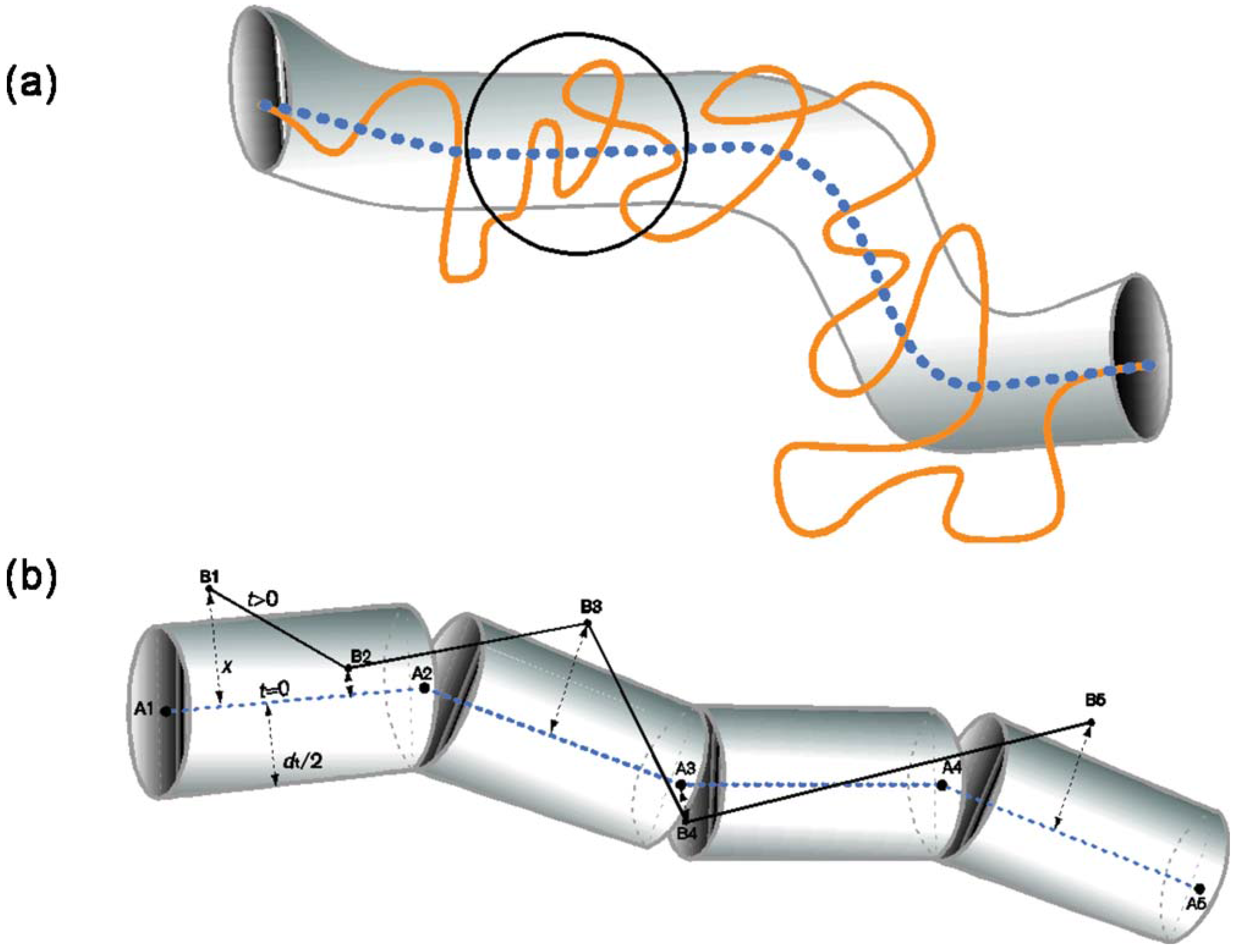
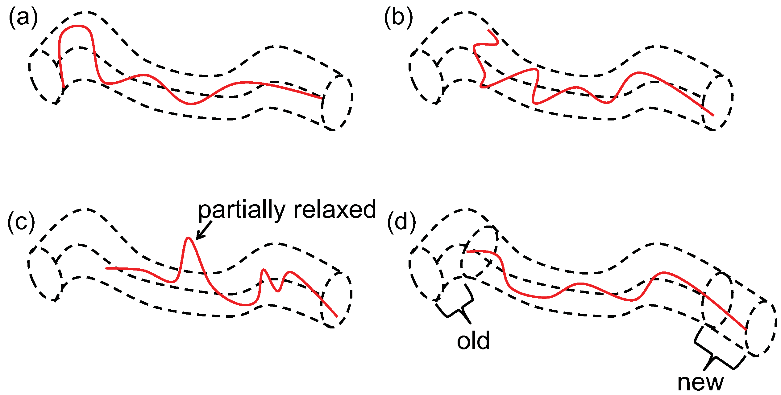
5.1. Dynamic Mapping onto Tube Model

Since the rheological properties of entangled polymer melts are dominated by entanglements, many computational works have been undertaken to extract the underlying primitive path (PP) and entanglement characteristics predicted by the tube model directly from the atomistic simulations [76,79,97,119,178,198,223,242,275,276,277,278,279,280,281,282,283,284,285]. All of the studies are based on the tube concept developed by Doi and Edwards [6] in which the PP is considered to be the shortest entanglement-preserving path between two ends of the polymer chain, as they are fixed in space. Everaers et al. [97,119] applied an energy-minimization method to extract a tube diameter and entanglement length from all-atomistic simulations of linear polymer chains. In this method, all the ends of the polymer chains are fixed in space. Then, most of the intra-chain interactions (vdW, angle and dihedral interactions) are turned off, while the inter-chain excluded volume interactions are retained. The bonded atoms or monomers only interact with each other through a FENE type potential. Afterward, the energy of the whole system is slowly minimized by cooling the system down to temperature, T = 0 K. The bond lengths and system energy are monitored in this process to ensure that the topological state of the PP network approaches a stationary value. Such a method is also referred to as the primitive path analysis (PPA) method [97,119]. Uchida et al. [120] combined computer simulations of the FENE model with bending, the PPA of the polymer topological state and scaling arguments to develop a unified picture of the relationship between plateau moduli and reduced polymer density. The obtained results agree with experimental observations of the normalized plateau moduli of both loosely and tightly entangled polymers over 13 decades in frequency space, from 10 - 6 to 10 7 s - 1 [120]. Recently, Everaers [286] compared the entanglement length, N e , given by the PPA, tube models and slip-link models, and proposed a simple relationship between topological and rheological entanglement length.
Within the original PPA method, the PP was defined as the path with minimum total energy, not as the shortest path between two ends of the chain, and PPA results are known to weakly depend on implementation details, such as a temperature ramp and bead size [276,287]. Later on, Kröger and Tzoumanekas et al. introduced the Z1 code [281,287] and contour reduction topological analysis (CReTA) [283] methods, respectively, to minimize the total contour length rather than the elastic energy, to supply a shortest parameter-free path for analyzing entanglement information of polymeric systems. Both Z1 and CReTA codes are purely geometric methods, which were found to give the same results on the same polymer systems [287]. The less computationally expensive Z1 code [279,281] begins to construct the PP network by fixing the ends of polymer chains and replacing each polymer chain by a series of infinitesimally thin, impenetrable and tensionless straight lines. The length of these multiple disconnected paths is then monotonically reduced, subject to chain-uncrossability, by introducing a smaller number of nodes. Upon iterating the procedure, each multiple disconnected path converges to a final state, the shortest path representing the PP. Recently, Schieber and his co-workers have developed an analytical expression for the PP length of entangled polymer chains [288,289,290], based on statistical mechanics of a chain as a random walk with randomly distributed entanglements. A single PP is often characterized by its conformational properties, i.e., PP length, L pp , number of interior kinks/entanglements, Z, and the end-to-end distance, R ee . According to the tube model [6], the real polymer chain and its corresponding PP both can be considered as random walks with the same R ee , but as different contour lengths. Thus, the tube diameter can be estimated as [6]:
a pp = R ee 2 L pp
Similarly, the entanglement length, N e , can be calculated via [6]:
N e = N R ee 2 L pp 2
while this expression for N e is generally N-dependent and requires simulations with N N e to determine N e precisely, there are also modified expressions that determine lower and upper bounds for N e . Most useful are the ideal N e -estimators that converge to N e for chain lengths, N N e . Such estimators are discussed in detail and tested by Hoy et al. [242].
Based on the Z1 code [281], Stephanou et al. [74,89,291,292,293] developed a dynamic mapping method to quantify polymer chain reptation in entangled polymer melts. As shown in Figure 17a, a virtual tube with diameter, a pp , is constructed around a real polymer chain and its PP, where the tube diameter, a pp , can be determined independently through either the calculation of the MSD for the innermost monomers of the polymer chains or the time displacement of the primitive chain segment orthogonal to the initial PP. As shown in Figure 17b, the tube is separated into consecutive cylinders. Here, each cylinder piece corresponds to an entanglement strand of the PP with a diameter, a pp . At time, t = 0 , the entanglement structure is A1-A2-A3-A4-A5, with each point representing a kink/entanglement along the PP. After time, t > 0 , the original polymer chain moves, as does its PP. The previous entanglement points thus move to a new configuration, which we denote as B1-B2-B3-B4-B5. The perpendicular distance traveled by each entanglement point, x ( s ) , can be calculated and compared with the tube radius, a pp / 2 . Here, s [ 0 , 1 ] labels the contour position of the PP segment. If x ( s ) > a pp / 2 , the segment, s, is considered to have escaped the initial tube perpendicularly, and the function, ψ ( s ) , whose average is taken over an ensemble of chains, describes the probability for the segment, s, to remain inside the original tube after time, t, is set to be 0. Conversely, if x ( s ) < a pp / 2 , the segment s has not laterally escaped the tube. However, we need to further check if it has escaped the tube longitudinally along the curvilinear axis. If not, ψ ( s ) = 1 . Such criteria work well for short times. However, for long time simulations, since the chain fluctuates and can retract back into its tube, these criteria are modified in accord with the tube theory [6]: (i) if x ( s ) < a pp / 2 , then ψ ( s , t ) = 1 ; (ii) if a pp / 2 < x ( s ) < a pp , then ψ ( s , t ) = 0 , but the segment is allowed to return back to its original tube; (iii) if x ( s ) > a pp , then ψ ( s , t ) = 0 , and the segment, s, cannot return to its original tube, which means ψ ( s , t ) = 0 for subsequent times, as well. Therefore, as shown in Figure 17b, we have ψ ( B 1 , t ) = 0 , ψ ( B 2 , t ) = 1 , ψ ( B 3 , t ) = 0 , ψ ( B 4 , t ) = 1 and ψ ( B 5 , t ) = 0 .
Figure 17. Schematic of tube construction around the primitive path (PP) of a polymer chain to calculate function, ψ ( s , t ) . Figure reproduced with permission from [89].
Polymers 05 00751 g017
Figure 18 shows successive illustrations of the instantaneous conformation of a reptating polymer chain with CR. For clarity, the conformations of a single chain are shown here. The movement of the chain and its PP can be clearly seen in Figure 18. It is obvious that the reptation behavior is not only due to the movement of the PP, but also due to fluctuations of the entanglements, which is accounted for by the CLF and CR effects. Specifically, the CR effect makes the main contribution to the relaxation of local transverse modes along the contour of PP, allowing some parts of the chain to explore the space outside of the average tube region for a certain time before disengagement (Figure 18c). These effects can be further enhanced by the thermally-induced local fluctuations perpendicular to the main PP orientation. As time goes on, more and more segments disengage the tube. Eventually, the entire chain can escape the original tube and form another new tube with its surrounding chains. As previously mentioned, the function, ψ ( s , t ) , can be obtained at any time, t, and averaged over all the chains in the system. As the molecular simulations can provide us with the atomistic trajectories at all times, these trajectories can be mapped onto the tube model by the Z1 code, as shown in Figure 3 in [89]. Therefore, the function, ψ ( s , t ) , can be numerically obtained from the molecular simulations combined with Z1 analysis. Moreover, to improve the statics, the multiple-time-origins technique is adopted during the calculation of ψ ( s , t ) . The portion of PP remaining inside its original tube after time, t, can be subsequently obtained as:
Ψ t = 1 L pp 0 L pp ψ s , t d s
The tube survivability function, Ψ t , is the key to the linear viscoelastic properties of polymers. The relaxation modulus reads [6]:
G t = G N 0 Ψ t
where G N 0 is the plateau modulus. In addition, the zero-rate shear viscosity, η 0 , and the storage, G ( ω ) , and loss, G ( ω ) , moduli can be obtained as [6]:
η 0 = 0 G t d t = G N 0 0 Ψ t d t
G ω = ω 0 G t sin ω t d t = G N 0 ω 0 Ψ t sin ω t d t
G ω = ω 0 G t cos ω t d t = G N 0 ω 0 Ψ t cos ω t d t
Here, we should emphasize that the tube survivability, Ψ t , is directly computed from the molecular simulations, without making any assumption aside from the tube concept. The original tube theory [6] provides a simple analytical expression for ψ s , t as ψ s , t = p : odd 4 / p π sin p π s / L pp exp - p 2 t / τ d , which implies the scaling behaviors, η 0 N 3 and D cm N - 2 , which, in fact, do not completely agree with experimental results [7,294], due to the inconsistency between the analytical expression of Ψ t and its true value.
Figure 18. Reptation behavior of a polymer chain with contour length fluctuation (CLF) and constraint release (CR) effects. The dashed center line represents the original primitive path, while the solid red line represents the actual polymer chain, whose instantaneous primitive path is not specifically indicated. The CLF effect is associated with the variation of the primitive path length resulting from the retraction and subsequent expansion of the polymer chain within the tube. The CR effect is illustrated by the polymer’s lateral escape from the tube in (c).
Polymers 05 00751 g018
Figure 19 shows the tube survivability, Ψ t , zero-rate shear viscosity, η 0 , and the storage, G ( ω ) , and loss, G ( ω ) , moduli of PE (C 500 H 1002 ) polymer melts at 450 K. In Figure 19a, the Ψ t is compared with the double reptation model [295,296] and dual constraint model [297,298]. Although all three of these models give similar trends in Ψ ( t ) , the double reptation model is found to overestimate the data obtained by direct PP analysis, due to the neglect of the CLF effect, while the dual constraint model is found to underestimate the data given by the PP analysis, due to the overestimation of CLF effect. Thus, there also exists some inconsistency for G ( ω ) and G ( ω ) between these three models, as shown in Figure 19c,d. Moreover, the zero-rate shear viscosities of PE melts obtained by the PP analysis are found to be in agreement with the experimental values, as given in Figure 19b. Baig et al. [74] utilized the same PP analysis method to study the dynamics of binary mixtures of entangled cis-1,4-PB melts and to explore the matrix chain length and composition effects of the CLF and CR mechanisms. Probe chains of C 600 cis-1,4-PB were immersed in matrices of varying chain lengths (from C 100 to C 1000 cis-1,4-PB). They found that the values of static topological properties, i.e., the average values of L pp and its fluctuation, did not change with different matrices. However, the different matrices have significant effects on the dynamical properties, i.e., ψ ( t , s ) , Ψ ( t ) , the time autocorrelation functions for L pp and the end-to-end unit vector [74]. As the length of the matrix chains decreases, the functions, ψ ( t , s ) and Ψ ( t ) , of probe chains are found to decrease more rapidly. Furthermore, the relaxation of longer chains is delayed as the concentration of shorter matrix chains decreases [74]. More importantly, the CR effect is found to be the dominant relaxation mechanism in the mixtures of longer and shorter cis-1,4-PB polymers, since the CLF effect appears to be independent of the compositional differences [74]. Later on, such a method was applied to improve the theoretical descriptions on the CLF and CR effects in the tube model [293].
Figure 19. Results of (a) tube survivability function, Ψ t ; (b) zero-rate shear viscosity, η 0 ; (c) storage, G ( ω ) , modulus; and (d) loss, G ( ω ) , modulus of PE (C 500 H 1002 ) polymer melts at 450 K. In (a), (c) and (d), the double reptation and dual constraint models are given by [295,296] and [297,298], respectively. In (b), the unfilled symbols are given by experiments. Figures reproduced with permission from [89].
Polymers 05 00751 g019

5.2. Molecularly-Derived Constitutive Equation

Recently, Ilg et al. [90,236,299,300,301] developed a molecularly-derived constitutive equation for low-molecular-weight FENE polymer melts from thermodynamically guided simulations and, also, applied similar concepts to sheared demixing systems [302], liquid crystals [303,304,305,306] and ferrofluids [307,308]. They have applied established concepts of non-equilibrium thermodynamics [309,310] and an alternating Monte-Carlo/molecular-dynamics scheme to derive a constitutive model for polymer melts under arbitrary flows (including shear and elongation). Here, we should emphasize that the molecularly-derived constitutive equation is based on a rigorous thermodynamics formulation, through an analytical super coarse-graining method. Therefore, it can be applied not only to generic polymers (i.e., FENE), but also polymers with chemical details; in fact, smaller-scale (i.e., MD or coarse-grained MD (CGMD)) simulation results are used as input. The issues of representability (associated with generic coarse-grained models) and transferability (associated with systematically coarse-grained models) in this method, therefore, arise from whatever smaller-scale model is chosen and can be avoided altogether by using an all-atomistic model as input. The main ingredient of this thermodynamically-guided method is the assumption that the non-equilibrium stationary state of the system is captured by a generalized canonical ensemble with the probability of state z being:
ρ z = f eq z e - Λ : Π z - Λ 0
where z = r j , p j are phase-space variables with r j and p j denoting particle positions and momenta, respectively. f eq z exp - H ( z ) / k B T , where H ( z ) represents the microscopic Hamiltonian. Λ ( x ) are Lagrange multipliers determined by the measured values of slow variables, x = Π z , and Λ 0 is a normalization constant. Here, the mesoscale behavior of the polymer melt is represented by the “structural” or “collective” variables, Π, which are assumed to be able to capture all the relevant physical processes on the time scale of interest. In their study, Ilg et al. chose the slow conformational variable to be the mean gyration tensor of polymer chains, considering that its decay is slow compared with fluctuations of bond lengths, angles and intermolecular distances or the higher normal modes [309,311]. The macroscopic hydrodynamic velocity field is ignored in Equation (31), since it equilibrates extremely rapidly on the length scale of individual polymer chains. Thus, the time evolution for the slow variables, x , can be written as [90]:
x ˙ = x ˙ rev + M : δ S δ x , δ S δ x = k B Λ
where x ˙ rev is the reversible contribution in terms of a Poisson bracket. The macroscopic entropy, S ( x ) = - k B ln ρ , is obtained with the distribution from Equation (31). The entropy gradient, δ S / δ x , determines the irreversible contribution through conjugation with M , a symmetric and semi-positive definite friction matrix obtained by a Green-Kubo type formula [309,312]:
M = M ( z ( t ) ) , M = 1 2 k B τ s Δ τ s Π ( z ) Δ τ s Π z
Here, Δ τ s Π ( z ) represents the fast fluctuation of Π on the time scale, τ s , which separates the evolution of the slow variables, x , from the rapid dynamics of the remaining degrees of freedom. The reversible part of the motion, x ˙ rev , can be obtained analytically by the transformation behavior of Π [309]. For example, as x represents the gyration tensor of polymer chains under homogeneous flow, v ( r ) = κ · r and κ = ( v ) T , one has x ˙ rev ( x , κ ) = x · κ T + κ · x . The remaining building blocks, Λ and M , can be determined self-consistently through a hybrid iteration scheme, as given below [90]:
  • Step (i): Choose initial values for the Lagrange multipliers, Λ
  • Step (ii): Generate n-independent configurations distributed according to the generalized canonical ensemble in Equation (31)
  • Step (iii): Solve Hamilton’s unconstrained equations of motion for all n systems during a short time interval, τ s
  • Step (iv): Calculate the friction matrix, M , from Equation (33) and x directly from the n trajectories produced in (iii)
  • Step (v): Calculate an updated value for Λ by solving Equation (32) for Λ with x ˙ = 0 (in terms of M , x and κ ; the transposed velocity gradient, κ , is “hidden” in x ˙ rev )
Note here the updated Lagrange multiplier obtained in step (v) can be used to reenter the procedure at step (i) for iteration, which will allow one to calculate the converged Λ. In step (ii), the Monte Carlo method is used to generate the equilibrated configurations for polymer chains with the same Lagrange multipliers used in step (i). In step (iii), NEMD simulations are performed on the configurations generated in step (ii) to calculate and store trajectories, z ( t ) , during a short time interval, t 0 , τ s . Here, we should emphasize that the duration of the MD simulation in step (iii) is very short, compared with conventional NEMD simulations, which should be larger than the inverse of the shear rate, γ ˙ - 1 . With all these n trajectories, z ( t ) , at hand, the friction term, M , can be evaluated in terms of the slow variables, Π ( z ( t ) ) , according to Equation (33) in step (iv). Here, the number of samples, n, should be large enough to obtain an accurate estimation of M . Afterward, Λ is updated according to Equation (32) and the value of M from step (iv). For a wide range of shear rates, γ ˙ - 1 , consistent sets of x , Λ ( x ) and M ( x ) can be obtained. The stress tensor of the polymer melt under shear flow can then be calculated as [90,299,313]
σ = - 2 n p k B T x · Λ
where n p is the polymer number density.
The above method can be applied to study both homogeneous, stationary flow situations for polymer melts and transient flows, as its implementation does not require flow-adapted periodic boundary conditions. Ilg and Kröger applied this method to study low-molecular-weight polymer melts under shear and other flows [299]. Figure 20 shows the transient behavior of FENE chains with N = 20 , under planar shear flow. For small shear rates, the transient viscosity, η + , increases monotonically and approaches its steady-state value for the strains, γ = γ ˙ t 1 . However, for large strain rates ( γ ˙ 10 - 2 , as shown in Figure 20a), there is an overshoot for η + before it reaches its stationary value. A similar behavior is also found for the transient first normal stress difference, Ψ 1 + = σ x x - σ y y , as shown in Figure 20b. These behaviors are experimentally observed [314,315] and have also been captured by different constitutive models [316,317]; however, these models tend to exhibit the inconvenient feature that they describe some types of flow very well, while failing for others [19]. In addition, the flow curves for η, Ψ 1 and the second normal stress difference, Ψ 2 = σ y y - σ z z , have been obtained and compare well with the NEMD results [299]. Baig and his co-workers [318,319] adopted a similar concept to study the viscoelasticity of polymer melts. They used an expanded Monte Carlo method as the macroscale solver for a family of viscoelastic models, which are built on the “structural” variable, x . Similar to the work done by Ilg et al. [90,299,313], x can be obtained from all-atomistic non-equilibrium simulations. Thus, there is no need to have an explicit form of the macroscopic model. The obtained conformation tensors, as well as the chain orientation functions of low-molecular weight PE melts are found to agree with atomistic non-equilibrium simulations [318].
Figure 20. (a) Normalized shear viscosity, η + / η 0 , and (b) normalized first normal stress coefficient, Ψ 1 + / Ψ 1 , 0 , for FENE chains with length N = 20 .
Polymers 05 00751 g020

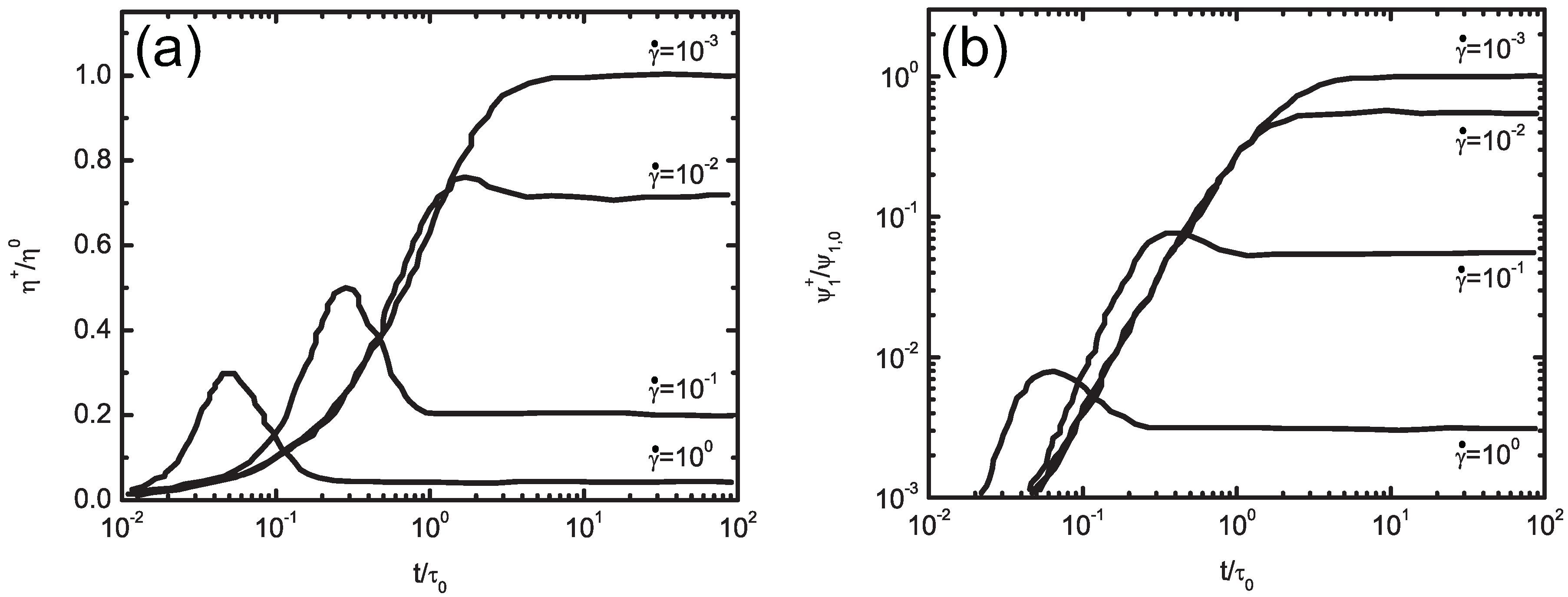
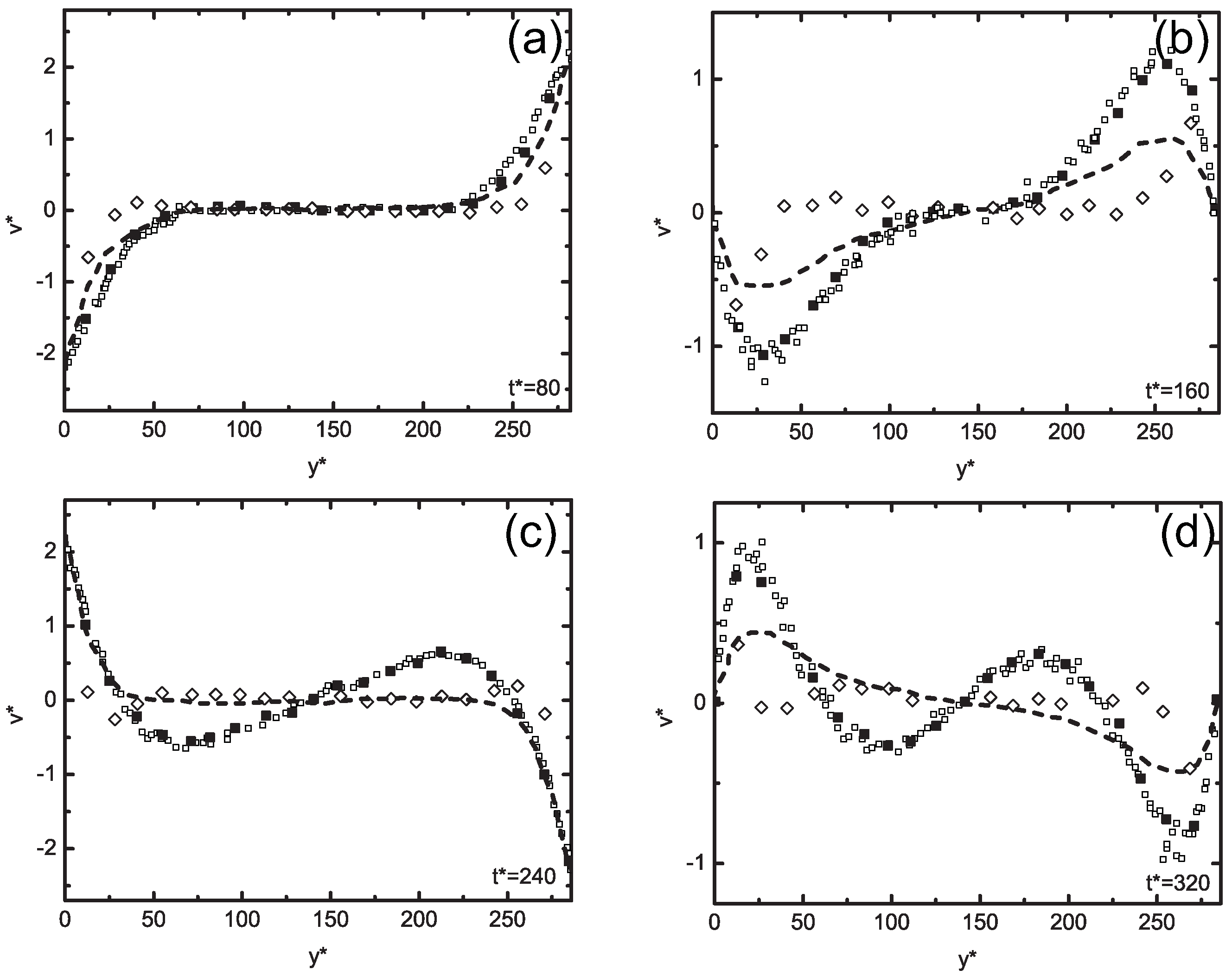
5.3. Concurrent Modeling of Polymer Melts under Shear Flow

Kumar and his co-workers developed a concurrent multiscale modeling strategy for parallel simulations of systems with a large spatial extent [91]. In this method, the continuum system is divided into multiple partitions. Each partition is simulated independently by MD simulations with periodic boundary conditions. Information is then occasionally passed between different partitions through a continuum approach without a constitutive model. The proposed method has been demonstrated in the simulation of polymer melts under rapid one-dimensional shear flow [91]. As shown in Figure 21, the polymer melt is subjected to a one-dimensional oscillatory shear flow along the x direction. The system is then partitioned along the y direction into N + 1 blocks. If we consider the entire system as a coarse-grained problem, it can be solved by determining the behavior at each Gauss point in the different partitions/blocks. As the Gauss-point behavior can be determined through independent NEMD simulations with the Lee-Edwards periodic boundary conditions [320], the coarse-grained problem should be easily solved. The velocity profile along the y direction from the coarse-grained problem serves as an input for the NEMD simulations of each Gauss point. The two scales are then coupled in a Lagrangian framework by following the generalized mathematical homogenization theory [321,322,323] for different scales:
m q ¨ x ζ - f x ζ = 0 for x ζ Θ ζ
ρ u ¨ ( x ζ ) - · σ ( x ζ ) = 0 for x ζ Ω
σ ( x ζ ) = 1 2 Θ ζ A B A r ζ AB x ζ f ζ AB x ζ
Equations (35) and (36) are for the fine scale (MD), scale bridging (modified virial stress) and the coarse scale (continuum), respectively. On the coarse scale, ρ is the density of the polymer melt, u ( x ) is the displacement vector in the continuum (coarse scale) and σ ( x ) is the Cauchy stress tensor in the continuum. On the fine scale (molecular level), q ( x ) is the displacement vector, m is the atomistic mass, r ζ AB is the radial vector between atoms A and B and f ζ AB is the force vector between atoms A and B. Ω represents the coarse domain, and Θ ζ represents the fine domain corresponding to the Gauss point, x ζ . From the above equations, we can see that the fine scale is governed by Newton’s second law with all the atomistic details and corresponding potentials. The stress tensor, σ ( x ) , at the Gauss point can be calculated based on the modified virial stress [321], which is further used as the input for the continuum equation of motion (on the coarse scale). The velocity field on the fine scale is updated according to the velocity field calculated on the coarse scale and used to run NEMD simulations in the next loop. Thus, σ ( x ) serves as the bridging law between the coarse-grained and fine-grained scales, and there is no need to use a constitutive model on the continuum scale. The NEMD simulations on the fine scale must be run for the duration of the time step used for the coarse grained integrator, Δ t . Moreover, the starting configurations for the NEMD simulations at Gauss points are taken as the ending configurations corresponding to the previous coarse-grained time step, which preserves the memory effect of friction.
The above method has been applied to study FENE chains with 120 beads per chain under oscillatory shear flow in the x direction. The velocity profiles along the y direction were monitored during the simulations (Figure 22). Reduced LJ units were used, and the period of oscillation was P * = 320 . The system temperature was kept at T 0 * = 1 by employing thermostats in the y and z directions. Obviously, at all times, the simulation results given by the proposed concurrent multiscale modeling method are in agreement with the results from the full MD simulations. When random starting configurations for each Gauss point were used, the obtained velocity profile was found to differ from the results of the full MD simulations, which addresses the importance of memory effects. Shear-thinning occurs in polymer melts under such high shear rates [324] and from the strain-rate dependent viscosity and its definition σ x y = η v x / y , the above coarse-grained problem can be directly solved without calculating the stress tensors in the fine scale at the Gauss points. However, the obtained velocity profile does not agree with the full MD simulations, due to anisotropy of chain conformation under such strong shear flow. The number of partitions can be adjusted in order to use the optimum number of Gauss points in the proposed approach, and the velocity profile can be linearly interpolated across the domain. The proposed method has been demonstrated to reproduce the velocity profile of full-fledged MD simulations, but with a net computational time gain proportional to the number of beads in the system, N bead (for large N bead ), thanks to the domain decomposition and parallelization [91]. The proposed concurrent method is similar in spirit to the above mentioned molecularly-derived constitutive equation, in that both of them require configurational inputs from full MD simulations. However, the concurrent method does not rely on a constitutive model on the continuum scale.
Figure 21. Description of the setup of the concurrent multiscale modeling method. The stresses calculated from MD simulations are passed into continuum simulation, while the velocity profile obtained from continuum simulations is used for the next set of MD simulations. Figure reproduced with permission from [91].
Polymers 05 00751 g021
Figure 22. The velocity profiles for the FENE system with thickness, 282σ, at different time steps. The small hollow and filled squares are given by the direct MD and concurrent multiscale simulations, respectively. The broken line is from the steady-state constitutive equation. The hollow diamonds are obtained from the concurrent multiscale simulations with equilibrated configurations freshly generated at each time. Figure reproduced with permission from [91].
Polymers 05 00751 g022

5.4. Hierarchical Modeling of Polymer Rheology

Very recently, Li et al. [92] developed a hierarchical multiscale method in which atomistic information is passed into a continuum constitutive model to predict the mechanical properties of linear polymers. The main idea in this hierarchical model is to decompose the material into two superimposed structures: a crosslinked (hyperelastic) network and a free-chain (viscous) network, as shown in the Figure 1 of [32]. The crosslinked network is characterized by its strand length, N elastic , and strand number density, n elastic , which primarily depend on the processing, e.g., how many crosslinkers are added and how the crosslinking occurs in polymers. Crosslinks are extremely strong chemical bonds that are unlikely to break under macroscopic deformation. The crosslinked network forms a relatively rigid internal frame that deforms in a homogeneous manner. The well-established Arruda-Boyce model [28,325,326] is used to describe the elastic behavior of the crosslinked network under deformation:
P E = W AB F - p J F - T
where P E is the elastic first Piola-Kirchhoff (PK1) stress, W AB is the hyperelastic internal energy, given in [28], F is the deformation gradient, p is the hydrostatic pressure and J det F . The viscous properties of polymers originate from the dynamic behavior of free chains. According to the tube model [5,6], assumed to describe the motion of these free chains, the viscous Cauchy stress can be formulated as [32]:
σ V = n v 3 k B T N b 2 L pp 2 0 t j = 1 , 3 , Υ ( j , t , t , τ d ) d t
where Υ is an integrand that depends on the tube survivability, Ψ ( t ) , and polymer chain rotation during deformation, as shown in [32,92]. The above viscous Cauchy stress can be related to its corresponding PK1 stress as J σ V = P V · F T [327]. The total stress response of the complex polymeric material under deformation is then the sum of the elastic stress tensor (Equation (38)) and the viscous stress tensor (Equation (39)). The parameters in the above equation fall into three categories: polymer chemistry, dynamics and physics. The chain length, N, and chain density, n v , represent the polymer chemistry of free chains, which also rely on the synthesis process. The polymer dynamics are represented by the diffusion coefficient, D cm , and disentanglement time, τ d , which can be obtained through experiments or MD simulations [92,328,329]. The tube diameter, a pp , PP length, L pp , and the Kuhn length, b, represent polymer physics, according to the tube model [5,6]. The Mittag-Leffler exponent, α, also represents polymer physics and enters through the modified tube survivability, Ψ ( t ) , which will be shown in the following section. The tube diameter, a pp , is related to the disentanglement time, τ d , which is also included in Ψ ( t ) . Through static PP analysis using Z1 code, all these parameters, except α, can be directly obtained [92,178,242,330]. The evaluation of α requires calibration with experimental results of the more sophisticated, dynamic PP analysis, whose description follows. In the molecular simulations, the trajectories of polymer chains can be directly mapped onto the tube model, through the Z1 code [89], as discussed in Section 5.1. Thus, the tube survivability, Ψ ( t ) , can be directly calculated, as shown in Figure 19a, which represents the portion of the primitive chain remaining inside the original tube after time, t. Afterward, the analytical equation for Ψ ( t ) obtained from the modified Doi-Edwards theory [32] with the Mittag-Leffler exponent, α, can be used to fit the numerical one obtained from molecular simulations. As such, all the parameters in the above constitutive model for the viscoelastic properties of polymers have physical meanings and can be directly predicted through the molecular simulations or experiments.
Figure 23 illustrates this multiscale computational framework developed to predict the viscoelastic properties of polymeric materials from the bottom up. The force field used in the all-atomistic simulations is obtained through quantum-mechanical calculations and, thus, acts as a bridging law between the pico- and nano-scales. The IBI method [37] then bridges the nano- and meso-scales by allowing us to coarse-grain the all-atomistic model. Applying the Z1 code [281] to the coarse-grained model, the PP network can be obtained and mapped onto the tube model, which bridges the meso- and micro-scales. Finally, through Equation (39), the tube model can be further utilized to derive the constitutive model for polymers in the macroscale. Since all the parameters in the macroscale constitutive model have physical meanings and can be obtained through coarse-grained molecular simulations and PP analysis [92], the viscoelastic properties of polymeric materials can be directly predicted from the bottom up without performing experiments. Vice versa, the developed hierarchical multiscale computational framework can also be applied in the parametric design of the viscoelastic properties of polymers, since all the parameters involved are signatures of polymer chemistry and physics.
Figure 23. Hierarchical multiscale computational framework adopted to predict the viscoelastic properties of polymers. Different time and length scales are connected through different bridging laws. Figure reproduced with permission from [92].
Polymers 05 00751 g023
The predicted storage ( G ) and loss ( G ) moduli of cis-PI polymer melts are given in Figure 24. Including the CLF and Rouse effects (see Appendix in [92]), the predicted moduli are in agreement with the experimental measurement for multiple molecular weights over a frequency range extending from 10 - 4 to 10 6 rad s - 1 (ten decades). For G in the terminal region, ω < τ d - 1 , we have G ω 2 . There is a sharp transition to the plateau region for G at higher frequencies. For extremely high frequencies ( ω > τ R - 1 ), G ω 1 / 2 in accord with the Rouse model [14,92,331]. Similarly, G ω in the terminal region, in accord with the tube model [6]. In the intermediate range ( τ d - 1 < ω < τ R - 1 ), the contribution of reptation to G is proportional to ω - 1 / 2 . However, the CLF effect will play an important role in this range, as discussed by McLeish and his co-workers [14,331]. In fact, G ω 1 / 4 in the intermediate range, due to the combined effects of reptation and CLF. In the high frequency range ( ω > τ R - 1 ), the polymer chain does not feel the constraint of its neighboring chains, thus G ω 1 / 2 , in line with the Rouse model [1]. As shown in Figure 24, the proposed hierarchical computational framework can both qualitatively and quantitatively capture all of these important features for cis-PI. In addition, the predicted G and G for PE (C 500 H 1002 ) also agree well with the atomistic simulations by Stephanou et al. [89] over a broad range of frequencies, ω [ 10 4 , 10 8 ] s - 1 , cf. Figure 10 of [92].
Figure 24. (a) Storage, G ; and (b) loss, G , moduli of cis-PI polymers with different molecular weights. The solid lines are given by the hierarchical multiscale computational framework. The dots are experimental results taken from [332]. Figure reproduced with permission from [92].
Polymers 05 00751 g024

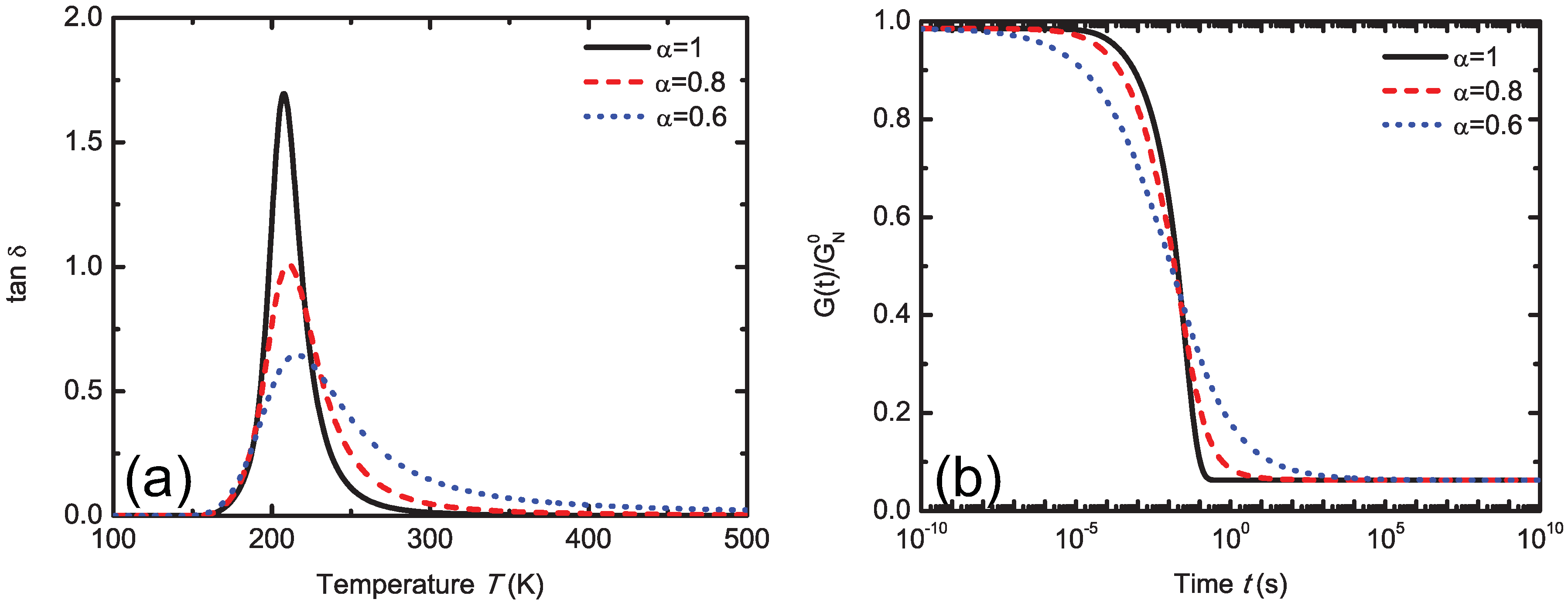
5.4.1. Mittag-Leffler Exponent α

The Mittag-Leffler exponent, α, plays an important role in the above multiscale computational framework. In the classical tube theory [6], the tube survivability, Ψ ( t ) , is known to follow from ψ ( s , t ) = p : odd 4 / p π sin p π s / L pp exp - p 2 t / τ d . However, this classical analytical equation does not agree well with the molecular observations, as shown in Figure 19a. Thus, the function, ψ ( s , t ) , was modified to take the form [32,92]:
ψ ( s , t ) = p = 1 , odd 4 p π sin p π s L pp E α , 1 - p 2 t τ d α
where the enhancement introduces the standard Mittag-Leffler function, E α , 1 , a solution to fractional diffusion problems. This introduces into the model a new parameter, α, that accounts for the effect of crosslinks or nonuniform distribution of molecular weight on relaxation (here, 0 α 1 ). Setting α = 1 reduces to the standard Doi-Edwards model [6], since E 1 , 1 ( x ) = exp ( x ) . Thus, the nature of the diffusive process is characterized by the Mittag-Leffler exponent, α, which indicates classical diffusion when equal to one, and anomalous (fractional) diffusion when between zero and one, leading to a widening of the glass transition and suppression of tan δ , as shown in Figure 25a. The width of the glass transition is also found to be proportional to 1 / α . The larger the value of α, the more uniform is the polymer’s relaxation spectrum, as shown in Figure 25b. Lion and Kardelky [333] applied a similar fractional diffusion equation to study the Payne effect in the finite viscoelasticity of carbon-black-filled elastomers.
Figure 25. Effect of the Mittag-Leffler exponent, α, on (a) tan δ and (b) the relaxation modulus, G ( t ) .
Polymers 05 00751 g025
Free-chain network polydispersity and interactions with the crosslinked network are the main causes of fractional diffusive behavior (α effect). To demonstrate this effect, the above multiscale computational framework with the enhancement of α has been applied to study the relaxation moduli G ( t ) of linear PE melts, as shown in Figure 26. If α = 1 , as suggested by the classical Doi-Edwards limit, the predicted G ( t ) can only capture the relaxation behavior of these polymers up to the disentanglement time, τ d . However, when t > τ d , the predicted G ( t ) is significantly smaller than the experimental one. Since the polydispersity index (PDI) of these PE samples is about 1.1 to 2.9 [92], the polymer chains should exhibit fractional diffusive behavior. Recall that α = 1 is for monodisperse polymer chains, which reduce Equation (40) to the standard Doi-Edwards model [6]. Thus, without the enhancement of α, the above multiscale computational framework cannot capture the correct relaxation behavior of these polydisperse chains. Since the PDI values of HPB TM polymersare rather small ( 1.1 ) [334], while they are as large as 1.8 to 2.9 for PEs [335], a large α = 0.7 value has been chosen for HPBs and a small one, α = 0.3 , for PEs when t > τ d . With the enhancement of α, the predicted G ( t ) is in agreement with experimental results, which further confirms the fractional diffusive behavior of polydisperse chains. A similar behavior has also been observed by Baig et al. [74]. They have calculated the tube survivability, Ψ ( t ) , of binary mixtures of entangled cis-1,4-PB melts. The decay of Ψ ( t ) for monodisperse C 600 cis-1,4-PB was very slow. However, the decay of Ψ ( t ) was sped up with increasing concentration of C 320 cis-1,4-PB inside the C 600 cis-1,4-PB matrix [74]. The observed decay of Ψ ( t ) is found to be in accordance with our previous speculations and discussions.
Figure 26. Normalized viscoelastic relaxation of various PE polymers at 463 K: (a) HPB TM and (b) PE. In (a), the dots are experimental results [334]. The solid and dash lines are given by the hierarchical method with α = 0.7 and 1.0 when t > τ d , respectively. In (b), the dots are experimental results [335]. The solid and dashed lines are from the hierarchical method with α = 0.3 and 1.0 when t > τ d , respectively. Figure reproduced with permission from [92].
Polymers 05 00751 g026

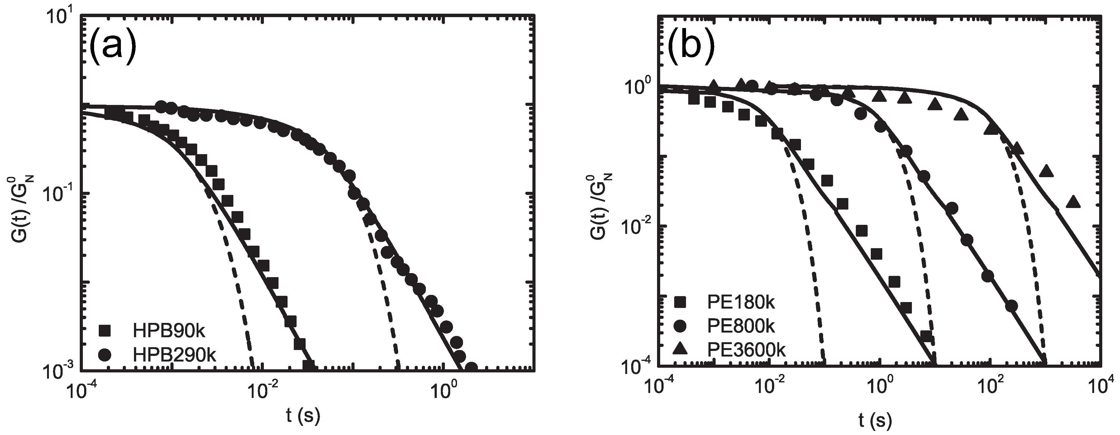
5.4.2. Finite Viscoelasticity Modeling

The developed multiscale computational framework can also be applied to the finite viscoelasticity of polymers. For example, consider the polymer bulk under one-dimensional tension with a stretch factor, λ = L / L 0 , with L and L 0 denoting the current and initial length of the material in the tension direction, respectively. The true strain is calculated as ln λ . Assuming the polymer is incompressible, the deformation gradient tensor, F , is:
F = 1 / λ 0 0 0 1 / λ 0 0 0 λ
and the unit vector, ν , tangent to the PP of a free chain is:
ν = 1 - z 2 cos ϕ 1 - z 2 sin ϕ z
where ϕ 0 , 2 π and z - 1 , 1 . Thus, according to the affine deformation assumption, we can calculate the deformed contour length of PPs as [6,336]:
L pp ( λ ) = L pp 0 F · ν d 2 ν = L pp 0 2 λ + sinh - 1 λ 3 - 1 λ 4 - λ
Assuming random walk statistics, the distribution of the end-to-end vector, R ee , in equilibrium is [6]:
f 0 ( R ee ) = 3 2 π N b 2 3 / 2 exp - 3 R ee 2 2 N b 2
where R ee 2 0 = N b 2 and b is the Kuhn length. The mean squared end-to-end distance, R ee 2 , in the deformed state is thus:
R ee 2 λ = F · R ee 2 f 0 R ee d 3 R ee = 2 + λ 3 3 λ R ee 2 0
and the change of tube diameter, a pp , is:
a pp λ a pp 0 = R ee 2 λ L pp λ L pp 0 R ee 2 0 = 2 2 + λ 3 3 λ λ + sinh - 1 λ 3 - 1 λ 4 - λ
The above derived Equations (43) and (46) are compared with molecular simulation results in Figure 27. A system of 200 FENE chains with N = 500 at number density ρ = 0.85 was extended under the canonical ensemble, at different strain rates and temperatures. The obtained trajectories were then analyzed with the Z1 code [281]. Obviously, the theoretical relationships between L pp or a pp and stretch ratio, λ, agree reasonably well with our molecular simulations, although the predicted L pp is larger than the simulation results at high temperature ( T = 1 ). Such differences imply the existence of non-affine deformation [26,337,338,339]. However, for chemically crosslinked polymers, i.e., vulcanized natural rubber, experimental results indicate that the deformation is affine [337]. Therefore, the proposed method should work well for finite deformation of chemically crosslinked polymers. The change of contour length, L pp , tube diameter, a pp , as well as the chain orientation have been considered in successful studies of the finite viscoelastic properties of polymeric materials [32,92]. As such, the proposed hierarchical multiscale computational framework captures both the linear and finite viscoelastic properties of polymeric materials well [32,92].
Figure 27. Uniaxial tension effect on (a) PP length, L pp , and (b) tube diameter, a pp , of FENE chains with length N = 500 . The dashed lines are given by Equations (43) and (46).
Polymers 05 00751 g027

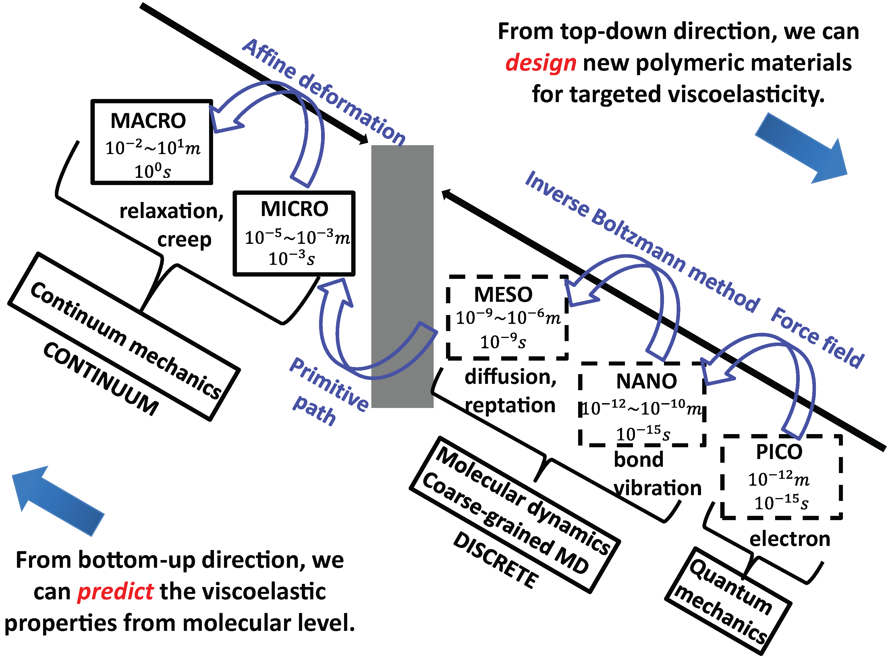
6. Perspectives and Challenges for Multiscale Modeling

6.1. From Atomistic to Macroscopic Scales and Back

The simulations reviewed in this paper were mostly performed independently at different spatial and temporal scales. The systematic coarse-graining methods, such as the IBI method, pass information from the all atomistic scale to the coarse-grained scale. Conversely, the well-equilibrated coarse-grained models can be mapped back onto an atomistic model, as reviewed by Müller-Plathe [38] and Peter and Kremer [340]. As the equilibration of a coarse-grained polymer is much faster and easier than the all-atomistic one, the back-mapping procedure can be used to quickly generate equilibrated all-atomistic models of highly entangled polymers, including polycarbonates [177,235,341], polystyrene [198,201] and polyamide [197,342]. Recently, Chen et al. [343] have extended this method to obtain polymer chains under non-equilibrium situations. In this back-mapping protocol, through applying position restraints on the deformed conformations of atactic polystyrene under steady-state shear flow, the atomistic details were reinserted. Such a back-mapping method presents an opportunity to study the atomistic details of highly entangled polymer chains under flow and their effect on measurable rheological quantities.
The multiple-scale-bridging methods enable the transfer of information from one scale to the next above, and so on. Most of these methods are hierarchical and transfer information in one direction. However, the concurrent modeling method reviewed in Section 5.3, borrowing ideas from the bridging scale method [344] and the bridging domain method [345], can exchange information and capture interaction between the fine scale and coarse scale in both directions. There is a tremendous amount of concurrent multiscale modeling methods developed in the recent ten years with rigorous mathematical foundations, but mostly for metals [344,346,347,348,349,350] and carbon nanomaterials [345,351,352,353,354]. These concurrent methods enable the information exchange between different length scales, capture their interactions and couple MD simulations with continuum simulations. Thus, both the atomistic details and the macroscopic properties of materials can be obtained at the same time from these simulations. In the future, if some of these methods can be extended to study polymeric materials, i.e., like the concurrent modeling method for polymers under shear flow [91], it will greatly enhance our understanding of their mechanical and physical properties, as well as our capability to design new materials.

6.2. Polymer Dynamics under Flow

Polymer melts under flow have distinct features, compared with Newtonian liquids, i.e., shear thinning and normal stress differences in shear flow [315,355], strain hardening in elongation [356] and shear banding [357]. All of these peculiar phenomena are related to the multiplicity of the temporal and spatial scales characterizing the structure and dynamics of polymer melts. Understanding the stress relaxation and the structural evolution over these multiple scales is a prerequisite for deriving a reliable constitutive model for polymer melts under shear flow. The only way to build the relationship between molecular structure, conformation, architecture and macroscopic rheology of polymer melts is through a comprehensive understanding across scales. Although recent MD simulation of FENE chains reproduces shear banding [358], it is a simple, brute-force approach. There is a demand today to move from such simple, brute-force computational experiments to complete, redundancy-free and consistent multiscale methods in studying the flow dynamics of polymeric materials. With help from recent advances in the field of non-equilibrium statistical mechanics and thermodynamics, the molecularly-derived constitutive equation, shown in Section 5.2, has demonstrated some capabilities in the comprehensive modeling of polymer flow behavior. However, the current results are limited to either generic polymer models (FENE chains [299]) or specific models of very simple polymers (PE chains [318]) with short chain length (smaller than or comparable to the entanglement length). Since the entanglements between different chains have significant effects on the dynamics and shear rheology of polymer melts, it is necessary to extend these methods to study the complex flow behavior of highly entangled polymer chains.
Applying the coarse-grained models developed under equilibrium conditions (i.e., IBI method) to flowing polymeric systems usually comes with some difficulties: the distinct time scales between the all-atomistic and coarse-grained models and the variation of the effective coarse-grained potential (e.g., the pair potential derived from the pair distribution under equilibrium conditions) with respect to the non-equilibrium flow field. Baig and Harmandaris [359] performed a quantitative analysis of a coarse-grained model for PS polymer melts under shear flow and compared the results with atomistic simulations. Both translational and orientational dynamics rescaling were applied to tackle the time scale issue. The dynamic properties of PS melts were reasonably captured by the coarse-grained model at low-to-intermediate strain rates, and the chain conformation was well reproduced by the coarse-grained model up to an intermediate flow strength (Weissenberg numbers W i < 10 ) [359]. However, the chain length in these studies was below the entanglement length. It is expected that such a method can be further extended to study entangled polymer chains subjected to flow.
Polymer flow in dilute solution is also an interesting and challenging problem [360]. Compared with polymer melts, particular attention must be paid to the solvent-mediation effect between polymeric beads, also called hydrodynamic interaction [361]. In order to avoid modeling the solvent explicitly, some techniques have been developed recently, such as dissipative particle dynamics [362], stochastic rotation dynamics [363,364] and the lattice Boltzmann method [365,366]. These methods not only provide an efficient and suitable coupling of the bead dynamics, but also the non-uniformities and fluctuations in the flow fields. Very recently, both the immersed finite element method [367] and the immersed boundary element method [368] have been extended to account for hydrodynamic interaction and thermal fluctuation in molecular or mesoscale simulations. However, most of the simulations for polymer flow in dilute or semi-dilute solutions incorporate simple mechanical models of polymers, i.e., dumbbell, FENE, bead-spring chain and bead-rod chain. Although these models can capture some important aspects of polymer dynamics and provide understanding of the key mechanisms, the obtained results still cannot be applied to specific polymers, as discussed when reviewing generic coarse-graining methods (Section 3). We further note that most of the concurrent methods reviewed in this paper are not capable of dealing with liquid solvents. The extension of the systematic coarse-graining and concurrent methods to study polymer flow in dilute solutions, taking into account full hydrodynamic interactions, thermal fluctuations and the properties of water and other solvents, is another area with its own challenges. While the relaxation time of polymer chains in dilute solutions is often small compared to that in concentrated or dense polymeric systems, and, thus, less obviously demanding for multiscale methods, the unapproximated calculation of long-ranged hydrodynamic interactions and detailed properties, such as hydrogen-bond structure of the solvent and its effect on polymer dynamics, has triggered its own area of research. For reviews see, e.g., [170,369].

6.3. Polymer Dynamics at Interfaces and in Interphases

The dynamic behavior of polymer chains close to a free surface or interface play a large role in predicting and designing the shear elasticity and viscosity of polymer nanocomposites (PNCs). For this reason, many computational and experimental works have been performed in recent years to understand the polymer dynamics at the interface and in the interphase [127,128,328,329,370,371,372,373,374,375,376,377,378,379,380,381,382]. While extensive works have been done to explore the chain dynamics inside PNCs, widely different and often conflicting results are reported. On the one hand, both experimental and computational results have suggested that a mobility gradient exists near the surface of nanoparticles (NPs) on a small, sub-chain-length scale [370,376,377]. On the other hand, silica NPs have been found to have no influence on the local segmental dynamics of poly(vinyl acetate) chains adjacent to them, when compared with the chains in the bulk [383]. Very recently, Richter and his co-workers carried out extensive neutron spin echo experiments on the dynamics of entangled polymer chains in PNCs [374,375,384]. For the polymer melts interacting with a confining surface, they found an anchored surface layer with internal high mobility, which was considered to be glassy in past works [370,376]. In addition, for poly(ethylene-alt-propylene) (PEP) matrices filled with hydrophobic (non-attractive) silica NPs, they reported several key findings [374,375]: (i) the Gaussian behavior of polymer chains was still preserved at a high volume fraction of NPs; (ii) NPs were found to have negligible influence on the basic Rouse relaxation rate of PEP chains; (iii) the effective lateral confining length of PEP chains increased with the NP volume fraction; (iv) a crossover from polymer chain entanglements to “NP entanglements” was observed with a critical NP volume fraction of about 35%; and (v) both the CLF and CR effects were suppressed by the appearance of NPs. All of these key findings, except (ii) and (v), were later observed by Li et al. [329] in large-scale isobaric MD simulations with generic NPs.
As discussed in this review, although many simulations have been applied to the polymer dynamics at interfaces, there is no conclusive answer to the question on how the dynamics of a polymer chain and its PP are affected by free surfaces or NPs. Most of the related works have utilized the generic coarse-grained polymer models, i.e., FENE chains. Thus, some of the key mechanisms in specific polymers may not be reproduced by these simulations. To address this issue, Bayramoglu and Faller [240] and Müller-Plathe and his co-workers [239,385] adopted a systematic coarse-graining method, the IBI method, to study confined polystyrene and Polyamide-6,6, respectively. Thus, in the future, we also expect to see that systematic coarse-graining methods, as discussed in Section 4, can be extended to study confined polymer dynamics in PNCs, which presents a great opportunity to understand the real situation of polymer dynamics at an interface or within an interphase. Such important understanding will enhance our capability to process and design PNCs with targeted mechanical and physical properties, as discussed extensively in [328,329,377,379,380,381,382,386,387,388,389,390,391].

6.4. Nonlinear Viscoelasticity, Viscoplasticity and Damage

Microstructured elastomeric solids have a broad range of applications, from blast-resistant shielding to vehicle tires. During deformation, these materials exhibit not only hyperelasticity, but also viscoelasticity, viscoplasticity and damage. These inelastic properties of elastomeric solids have a large impact on functionality. For example, when the rubber compounds filled with carbon black are under cyclic loading conditions with small strain amplitudes, the storage modulus is found to rapidly decrease as the strain amplitude increases. Such a behavior is the so-called “Payne effect” [392,393], which is attributed to the deformation-induced change of the internal microstructure of elastomeric solids, i.e., the breakage and recovery of weak physical bonds between carbon black clusters. This effect is also essential for the frequency and amplitude-dependent dynamic mechanical properties and damping behavior of tire compounds. Several constitutive models [333,394] have been developed to characterize this important feature, incorporating the concept of occlusion to account for the breakage of weak physical bonds. However, the underlying assumptions have not been rigorously tested against the existing experiments or simulations; the models remain purely phenomenological. This situation can be improved by applying multiscale computational techniques to study microstructural evolution during deformation. The corresponding insights will help to develop a predictive constitutive model with solid physical mechanisms for designing microstructured elastomeric solids [32,395].
In the viscoplastic deformation of polymer glasses, strain hardening plays an important role in stabilizing polymers against strain localization and fracture. The entropic network models [396,397], based on the rubber elasticity theory, produce good fitting to experimental data. However, the underlying assumptions in these theoretical models are found to be inconsistent with the molecular simulations [121,122,123]. For example, when the segments between entanglements are pulled taut, the corresponding energy contribution to the stress grows rapidly [122]. Moreover, when the stresses are plotted against the microscopic strain-induced chain orientation ( g ( λ eff ) λ eff 2 - 1 / λ eff , where λ eff denotes the average stretch ratio of the end-to-end distance of polymer chains), instead of the macroscopic strain (stretch ratio, λ), both entangled and unentangled chains show the same strain hardening behavior, which cannot be explained by the entropic network models. Hoy and Robbins [121] studied the effects of entanglement density, temperature and deformation rate on the strain hardening behavior of polymer glasses. They found that the dependence of strain hardening on strain and entanglement density was consistent with these entropic network models, while the temperature dependence showed the opposite trend. They also studied the change of PP length, L pp , and tube diameter, a pp , of polymer glasses with deformation, which can be fitted using the mean-field tube model. Similar to the case of viscoelasticity, these studies are still limited to the generic coarse-grained polymer model. However, they are also expected to be extendable to the systematic coarse-graining models or the multiple-scale-bridging methods to investigate the viscoplastic deformation mechanisms of polymer glasses.
When a pre-cracked particle-reinforced elastomer specimen with a 4 × 5 mm 2 cross-section was loaded in tension, Akutagawa et al. [398] found a highly localized strain region near the crack tip in a roughly circular area with diameter 0.5 mm. They utilized 3D transmission electron microtomography to extract a digital data set and reconstructed the microstructure of filler networks, as shown in Figure 28a. When the applied global strain was about 15%, they found a strikingly high strain concentration, about 200%, between the fillers. Thus, strain localization can be thirteen-times greater than the applied overall strain, which can induce fracture and damage of particle-reinforced elastomers. It seems therefore crucial to properly capture the post-localization phenomena in the continuum modeling of microstructured viscoelastic materials in order to predict the initiation and propagation of the fracture path [395]. Very recently, Tang et al. [32] developed a two-scale multiresolution continuum theory to study strain localization in filled elastomers. With damaged elements introduced into the continuum simulation, they demonstrated that the proposed two-scale theory can qualitatively capture strain localization and corresponding stress softening phenomena, as illustrated in Figure 28b. When the applied global strain was 0.2, the maximum local strain was found to be about 0.7, which is more than three-times the applied strain. This agrees with the three- to 13-fold strain localization observed in the experiments [398,399]. However, the current studies on damage and strain softening phenomena are mostly limited to continuum modeling [32,333,395,400,401]. Greater predictive power can be achieved if multiscale computational techniques are applied to study the molecular and mesoscopic mechanisms related to damage and strain softening phenomena.
Figure 28. Strain amplification in filled elastomers under tension: (a) experimental and (b) computational results. The green/yellow and red colors in (a) and (b), respectively, correspond to high strain localization regions. Parts (a) and (b) reproduced with permission from [32,398], respectively.
Polymers 05 00751 g028

7. Summary and Conclusions

The structure and dynamics of polymeric materials involve multiple length and time scales. It is unfeasible to use a single computer simulation method to capture all of their relevant aspects. Rather, it is necessary to adopt a multiscale computational technique to study polymeric materials at spatial and temporal scales that span several orders of magnitude. In this review, we have divided the different multiscale modeling methods into three categories: (i) coarse-graining methods for generic polymers; (ii) systematic coarse-graining methods; and (iii) multiple-scale-bridging methods. In the coarse-graining methods (i) for generic polymers, the simulations are performed on the length scale of the Kuhn or entanglement length, without considering detailed chemical structures. These methods can provide us with an understanding of the key mechanisms of polymeric materials and their interplay within relatively large time and length scales (Section 3). However, due to the lack of detailed chemical information, the obtained results do not provide quantitative predictions for the relaxation dynamics of specific polymers, unless the involved simulation units can be calibrated to match a particular chemistry. To overcome this issue, systematic coarse-graining methods (ii) were developed from all-atomistic models. In these methods, a few atoms are lumped into a single super atom. According to the degree of coarse-graining, the systematic coarse-graining methods can be further divided into the IBI method, the blob model and the super coarse-graining method (Section 4). Within the IBI method, one or two monomers are coarse-grained into one super atom. Therefore, the underlying entanglement network of polymers can be well captured with a computational speedup of two orders of magnitude, compared with all-atomistic methods (Section 4.1). In the blob model, about twenty monomers are coarse-grained into one super atom. To preserve the important aspect of chain uncrossability in the blob model, extra bond interactions are introduced (Section 4.2). Similar to the coarse-graining methods in Category (i), the acceleration of this method is about three or four orders of magnitude compared with all-atomistic simulations. To reach an even higher degree of coarse-graining, the entire polymer chain can be coarse-grained into a soft colloidal particle with the super coarse-graining method (Section 4.3). The friction and stochastic interactions play important roles in the dynamics of these colloids. The super coarse-grained model can provide accurate predictions of some dynamic and rheological properties of polymer melts with a computational speedup of roughly six orders of magnitude, compared with all-atomistic methods.
On the basis of these coarse-grained simulations, different computational techniques for different scales can be coupled together in the multiscale modeling of polymeric materials, with the help of different bridging laws, as in the multiple-scale-bridging methods (iii). In the dynamical mapping method (Section 5.1), the trajectories of polymer chains are mapped onto the tube model upon invoking a primitive path analyzer. This way, the tube survivability can be directly quantified from the MD simulations. It is further used to calculate the storage and loss moduli, relaxation modulus and shear viscosity of polymers. The calculated tube survivability was used to test the double reptation and dual constraint models. The dual constraint model is found to overestimate the degree of polymer chain relaxation (lower survivability and modulus), while the double reptation model underestimates it (higher survivability and modulus). The dynamical mapping method can help to verify or reject the assumptions of different theoretical models and to provide insight into the physical mechanisms that should be incorporated into future theoretical models. Following the concept of non-equilibrium steady states, a molecularly-derived constitutive equation was developed to study the macroscopic properties of polymer melts subject to homogeneous flows (Section 5.2). This constitutive model is informed by detailed MD simulations, within rigorous non-equilibrium statistical mechanics and thermodynamics frameworks and captures both the linear and nonlinear rheology of unentangled polymer melts.
Using the macroscopic Cauchy stress calculated from the virial stress in MD simulations, the macroscopic velocity profile can be updated through a continuum approach without a constitutive model (Section 5.3). This velocity profile can then be used for the next set of MD simulations. Such a concurrent modeling method has been applied to study one-dimensional polymer flow in shear. The obtained velocity profile is in agreement with the full MD simulations. In contrast to the concurrent method, Li et al. developed a hierarchical multiscale modeling method to study the viscoelastic properties of polymeric materials (Section 5.4). In this method, the information from the all-atomistic scale is passed to the macroscopic constitutive model to directly predict viscoelastic properties. The different scales are coupled by bridging rules. For example, the IBI method is applied to bridge the scale from all-atomistic to the coarse-grained scale, and primitive path analysis (Z1 code) is then used to take the information from the coarse-grained scale to the microscale (tube model) (Figure 23). The proposed hierarchical multiscale modeling method can be applied to study both the linear and nonlinear viscoelasticity of polymers.
Perspectives and remaining challenges in the multiscale modeling of polymeric materials are discussed extensively in Section 6. Is it possible to pass the information from the atomic to macroscopic scale and back? Can a back-mapping scheme be applied to study polymer melts under strong shear flow? Can we extend the existing concurrent modeling methods for metals and carbon nanomaterials to polymeric and composite systems? Why do shear thinning and normal stress differences occur in shear flow, but strain hardening in elongation? Why and how does shear banding develop in unentangled and entangled polymers? Can we use the multiscale modeling methods to describe polymer flow in dilute and concentrated solutions? How does the free surface and interface affect the dynamical behavior of polymer chains and their underlying PP networks? Is there a glassy polymer layer near the surface of NPs in PNCs? What are the molecular origins for the viscoelasticity, viscoplasticity and damage in filled elastomers? How can we use the multiscale modeling techniques to characterize these phenomena? Can the concept of non-equilibrium steady states also be used to develop constitutive equations for entangled polymer melts? Can the super coarse-grained methods be extended to describe phenomena, such as flow birefringence? These questions are just a few among a vast number of topics for the future research of polymeric materials that have not, or have only to some extent, been addressed, so far. With continuous progress in simulation and experimental techniques, answering these questions will lead to a comprehensive understanding and description of the mechanical and physical properties of polymeric materials across different spatial and temporal scales. It will also guide us to design new polymeric materials with desired or yet unexplored properties in the future.
Nomenclature
definitions are given here in the following sequence: Roman alphabetical order followed by Greek alphabetical order. Bold quantities denote vectors or tensors.
a pp
tube diameter in reptation/tube model
a T
shift factor in time-temperature superposition principle
b
Kuhn length of polymer chain as R ee 2 = N b 2
D cm
self-diffusion coefficient of polymer chain
D Rouse
diffusion coefficient defined by the Rouse model as D Rouse = k B T / N ζ
G , G
storage and loss shear moduli
G N 0 , G ( t )
plateau and relaxation shear moduli
F
deformation gradient tensor
L, L 0
current and initial length of material in the direction of uniaxial tension
L pp
primitive chain length in reptation/tube model, defined as L pp = R ee 2 / a pp
M RI
geometric mapping matrix between all-atomistic and coarse-grained models
N
number of monomers per chain
N e
entanglement length, which is the number of monomers between two entanglements
n v
number of polymer chains per unit volume
n i j n 0 ( r i j )
entanglement number (at equilibrium) between particle pairs i and j
p r , P R
configurational probability distributions in all-atomistic and coarse-grained models, respectively
R ee
end-to-end distance of polymer chain
R G
radius of gyration of polymer chain
s
segment index/contour length variable along primitive chain
S ( q )
single chain coherent dynamic scattering function
Z
number of entanglements per chain, defined as Z = N / N e
α
exponent in standard Mittag-Leffler function
σ E
elastic part of Cauchy stress
σ V
viscous part of Cauchy stress
P E
elastic part of nominal stress
P V
viscous part of nominal stress
η , η 0
viscosity and zero-rate viscosity
γ, γ ˙
shear strain and shear strain rate
λ
stretch ratio in uniaxial tension, defined as λ = L / L 0
ν
unit tangent vector of the primitive chain
ω
circular frequency
ψ ( s , t )
probability that chain segment, s, remains in the tube of reptation at time, t
Ψ ( t )
tube survivability function, defined as Ψ ( t ) = 0 L pp ψ s , t d s / L pp
τ d
disentanglement time of polymer chain, defined as τ d = L pp 2 / π 2 D cm
τ e
entanglement time of polymer chain, defined as τ e = ( 1 / 3 ) τ d / ( N / N e ) 3
τ R
Rouse time of polymer chain, defined as τ R = ( 1 / 3 ) τ d / ( N / N e )
ζ
friction coefficient between polymer beads
ζ AA , ζ CG
friction coefficients in all-atomistic and coarse-grained models, respectively

Acknowledgments

This work was supported by NSF CMMI Grants 0823327, 0928320 and NSF IDR Grant 1130948. Y. Li acknowledges partial financial support from the Ryan Fellowship at Northwestern University. W.K. Liu was also partially supported by the World Class University Program through the National Research Foundation of Korea (NRF) funded by the Ministry of Education, Science and Technology (R33-10079). This research used resources of the QUEST cluster at Northwestern University and the Argonne Leadership Computing Facility at Argonne National Laboratory, which is supported by the Office of Science of the U.S. Department of Energy under contract DE-AC02-06CH11357. We acknowledge valuable comments from anonymous reviewers.

References

  1. Rouse, P.E., Jr. A theory of the linear viscoelastic properties of dilute solutions of coiling polymers. J. Chem. Phys. 1953, 21, 1272–1280. [Google Scholar] [CrossRef]
  2. Mondello, M.; Grest, G.S.; Webb, E.B.; Peczak, P. Dynamics of n-alkanes: Comparison to Rouse model. J. Chem. Phys. 1998, 109, 798–805. [Google Scholar] [CrossRef]
  3. Harmandaris, V.A.; Doxastakis, M.; Mavrantzas, V.G.; Theodorou, D.N. Detailed molecular dynamics simulation of the self-diffusion of n-alkane and cis-1, 4 polyisoprene oligomer melts. J. Chem. Phys. 2002, 116, 436–446. [Google Scholar] [CrossRef]
  4. Fleischer, G.; Appel, M. Chain length and temperature dependence of the self-diffusion of polyisoprene and polybutadiene in the melt. Macromolecules 1995, 28, 7281–7283. [Google Scholar] [CrossRef]
  5. De Gennes, P.G. Scaling Concepts in Polymer Physics; Cornell University Press: Ithaca, NY, USA, 1979. [Google Scholar]
  6. Doi, M.; Edwards, S.F. The Theory of Polymer Dynamics; Oxford University Press: New York, NY, USA, 1988; Volume 73. [Google Scholar]
  7. McLeish, T.C.B. Tube theory of entangled polymer dynamics. Adv. Phys. 2002, 51, 1379–1527. [Google Scholar] [CrossRef]
  8. Doi, M. Explanation for the 3. 4-power law for viscosity of polymeric liquids on the basis of the tube model. J. Polym. Sci. Polym. Lett. 1983, 21, 667–684. [Google Scholar] [CrossRef]
  9. Needs, R.J. Computer simulation of the effect of primitive path length fluctuations in the reptation model. Macromolecules 1984, 17, 437–441. [Google Scholar] [CrossRef]
  10. Watanabe, H. Viscoelasticity and dynamics of entangled polymers. Progr. Polym. Sci. 1999, 24, 1253–1403. [Google Scholar] [CrossRef]
  11. Schweizer, K.S.; Curro, J.G. Integral equation theories of the structure, thermodynamics, and phase transitions of polymer fluids. Adv. Chem. Phys. 1997, 98, 1–142. [Google Scholar]
  12. Schweizer, K.S.; Fuchs, M.; Szamel, G.; Guenza, M.; Tang, H. Polymer-mode-coupling theory of the slow dynamics of entangled macromolecular fluids. Macromol. Theory Simul. 1997, 6, 1037–1117. [Google Scholar] [CrossRef]
  13. Dealy, J.M.; Larson, R.G. Structure and Rheology of Molten Polymers: From Structure to Flow Behavior and Back again; Hanser Gardner Publications: Heidelberg, Germany, 2006. [Google Scholar]
  14. Likhtman, A.E.; McLeish, T.C.B. Quantitative theory for linear dynamics of linear entangled polymers. Macromolecules 2002, 35, 6332–6343. [Google Scholar] [CrossRef]
  15. Hou, J.X.; Svaneborg, C.; Everaers, R.; Grest, G.S. Stress relaxation in entangled polymer melts. Phys. Rev. Lett. 2010, 105, 068301:1–068301:4. [Google Scholar] [CrossRef]
  16. Kröger, M. Simple models for complex nonequilibrium fluids. Phys. Rep. 2004, 390, 453–551. [Google Scholar] [CrossRef]
  17. Larson, R.G.; Zhou, Q.; Shanbhag, S.; Park, S.J. Advances in modeling of polymer melt rheology. AIChE J. 2007, 53, 542–548. [Google Scholar] [CrossRef]
  18. Likhtman, A.E. Viscoelasticity and Molecular Rheology. In Comprehensive Polymer Science; Elsevier: Amsterdam, The Netherlands, 2011. [Google Scholar]
  19. Fang, J.; Kröger, M.; Öttinger, H.C. A thermodynamically admissible reptation model for fast flows of entangled polymers. II. Model predictions for shear and extensional flows. J. Rheol. 2000, 44, 1293–1317. [Google Scholar] [CrossRef]
  20. Shanbhag, S. Analytical rheology of polymer melts: State of the art. ISRN Mater. Sci. 2012, 2012, 732176:1–732176:24. [Google Scholar] [CrossRef]
  21. Edwards, S.F.; Vilgis, T.A. The tube model theory of rubber elasticity. Rep. Progr. Phys. 1999, 51, 243–297. [Google Scholar] [CrossRef]
  22. Edwards, S. The statistical mechanics of polymerized material. Proc. Phys. Soc. 1967, 92, 9–16. [Google Scholar] [CrossRef]
  23. Edwards, S. Statistical mechanics with topological constraints: I. Proc. Phys. Soc. 1967, 91, 513–519. [Google Scholar] [CrossRef]
  24. Edwards, S. Statistical mechanics with topological constraints: II. J. Phys. A 1968, 1, 15–28. [Google Scholar] [CrossRef]
  25. De Gennes, P.G. Reptation of a polymer chain in the presence of fixed obstacles. J. Chem. Phys. 1971, 55, 572–579. [Google Scholar] [CrossRef]
  26. Rubinstein, M.; Panyukov, S. Nonaffine deformation and elasticity of polymer networks. Macromolecules 1997, 30, 8036–8044. [Google Scholar] [CrossRef]
  27. Rubinstein, M.; Panyukov, S. Elasticity of polymer networks. Macromolecules 2002, 35, 6670–6686. [Google Scholar] [CrossRef]
  28. Arruda, E.M.; Boyce, M.C. A three-dimensional constitutive model for the large stretch behavior of rubber elastic materials. J. Mech. Phys. Solids 1993, 41, 389–412. [Google Scholar] [CrossRef]
  29. Miehe, C.; Göktepe, S.; Lulei, F. A micro-macro approach to rubber-like materials. Part I: The non-affine micro-sphere model of rubber elasticity. J. Mech. Phys. Solids 2004, 52, 2617–2660. [Google Scholar] [CrossRef]
  30. Miehe, C.; Göktepe, S. A micro–macro approach to rubber-like materials. Part II: The micro-sphere model of finite rubber viscoelasticity. J. Mech. Phys. Solids 2005, 53, 2231–2258. [Google Scholar] [CrossRef]
  31. Göktepe, S.; Miehe, C. A micro–macro approach to rubber-like materials. Part III: The micro-sphere model of anisotropic Mullins-type damage. J. Mech. Phys. Solids 2005, 53, 2259–2283. [Google Scholar] [CrossRef]
  32. Tang, S.; Greene, M.S.; Liu, W.K. Two-scale mechanism-based theory of nonlinear viscoelasticity. J. Mech. Phys. Solids 2012, 60, 199–226. [Google Scholar] [CrossRef]
  33. Jensen, M.K.; Khaliullin, R.; Schieber, J.D. Self-consistent modeling of entangled network strands and linear dangling structures in a single-strand mean-field slip-link model. Rheol. Acta 2012, 51, 21–35. [Google Scholar] [CrossRef]
  34. Gee, R.H.; Lacevic, N.; Fried, L.E. Atomistic simulations of spinodal phase separation preceding polymer crystallization. Nat. Mater. 2005, 5, 39–43. [Google Scholar] [CrossRef] [PubMed]
  35. Baschnagel, J.; Binder, K.; Doruker, P.; Gusev, A.; Hahn, O.; Kremer, K.; Mattice, W.; Müller-Plathe, F.; Murat, M.; Paul, W.; et al. Bridging the Gap between Atomistic and Coarse-grained Models of Polymers: Status and Perspectives. In Viscoelasticity, Atomistic Models, Statistical Chemistry; Springer: Berlin, Germany, 2000; pp. 41–156. [Google Scholar]
  36. Kremer, K.; Müller-Plathe, F. Multiscale simulation in polymer science. Mol. Simul. 2002, 28, 729–750. [Google Scholar] [CrossRef]
  37. Faller, R. Automatic coarse graining of polymers. Polymer 2004, 45, 3869–3876. [Google Scholar] [CrossRef]
  38. Müller-Plathe, F. Coarse-graining in polymer simulation: From the atomistic to the mesoscopic scale and back. ChemPhysChem 2002, 3, 754–769. [Google Scholar] [CrossRef]
  39. Müller-Plathe, F. Scale-hopping in computer simulations of polymers. Soft Mater. 2002, 1, 1–31. [Google Scholar] [CrossRef]
  40. Paul, W.; Smith, G.D. Structure and dynamics of amorphous polymers: Computer simulations compared to experiment and theory. Rep. Progr. Phys. 2004, 67, 1117–1185. [Google Scholar] [CrossRef]
  41. Padding, J.T.; Briels, W.J. Systematic coarse-graining of the dynamics of entangled polymer melts: The road from chemistry to rheology. J. Phys. Condens. Matter 2011, 23, 233101:1–233101:17. [Google Scholar] [CrossRef] [PubMed]
  42. Karimi-Varzaneh, H.A.; van der Vegt, N.F.A.; Müller-Plathe, F.; Carbone, P. How good are coarse-grained polymer models? A comparison for atactic polystyrene. ChemPhysChem 2012, 13, 3428–3439. [Google Scholar] [CrossRef] [PubMed]
  43. Brini, E.; Algaer, E.A.; Ganguly, P.; Li, C.; Rodríguez-Ropero, F.; van der Vegt, N.F. Systematic coarse-graining methods for soft matter simulations—A review. Soft Matter 2013, 9, 2108–2119. [Google Scholar] [CrossRef]
  44. Holm, C.; Kremer, K. Advanced computer simulation approaches for soft matter sciences I. Adv. Polym. Sci. 2005, 173, 1–275. [Google Scholar]
  45. Holm, C.; Kremer, K. Advanced computer simulation approaches for soft matter sciences II. Adv. Polym. Sci. 2005, 185, 1–250. [Google Scholar]
  46. Holm, C.; Kremer, K. Advanced computer simulation approaches for soft matter sciences III. Adv. Polym. Sci. 2009, 221, 1–237. [Google Scholar]
  47. Voth, G.A. Coarse-Graining of Condensed Phase and Biomolecular Systems; CRC Press: Cambridge, UK, 2009. [Google Scholar]
  48. Faller, R. Biomembrane Frontiers: Nanostructures, Models, and the Design of Life; Springer: Berlin, Germany, 2009; Volume 2. [Google Scholar]
  49. Scheutjens, J.M.H.M.; Fleer, G.J. Statistical theory of the adsorption of interactingchain molecules. 1. Partition-function, segment density distribution, and adsoprtion-isotherms. J. Phys. Chem. 1979, 83, 1619–1635. [Google Scholar] [CrossRef]
  50. Boris, D.; Rubinstein, M. A self-consistent mean field model of a starburst dendrimer: Dense core vs. dense shell. Macromolecules 1996, 29, 7251–7260. [Google Scholar] [CrossRef]
  51. Lai, P.Y.; Binder, K. Structure and dynamics of polymer brushes near the theta point-A Monte Carlo simulation. J. Chem. Phys. 1992, 97, 586–595. [Google Scholar] [CrossRef]
  52. Szleifer, I.; Carignano, M.A. Tethered polymer layers. Adv. Chem. Phys. 1996, 94, 165–260. [Google Scholar]
  53. Detcheverry, F.A.; Kang, H.M.; Daoulas, K.C.; Müller, M.; Nealey, P.F.; de Pablo, J.J. Monte Carlo simulations of a coarse grain model for block copolymers and nanocomposites. Macromolecules 2008, 41, 4989–5001. [Google Scholar] [CrossRef]
  54. Zhulina, E.B.; Wolterink, J.K.; Borisov, O.V. Screening effects in a polyelectrolyte brush: Self-consistent-field theory. Macromolecules 2000, 33, 4945–4953. [Google Scholar] [CrossRef]
  55. Müller, M. Phase diagram of a mixed polymer brush. Phys. Rev. E 2002, 65, 030802:1–030802:4. [Google Scholar] [CrossRef]
  56. Stuart, M.A.C.; Huck, W.T.S.; Genzer, J.; Müller, M.; Ober, C.; Stamm, M.; Sukhorukov, G.B.; Szleifer, I.; Tsukruk, V.V.; Urban, M.; et al. Emerging applications of stimuli-responsive polymer materials. Nat. Mater. 2010, 9, 101–113. [Google Scholar] [CrossRef] [PubMed]
  57. Halperin, A.; Kröger, M. Theoretical considerations on mechanisms of harvesting cells cultured on thermoresponsive polymer brushes. Biomaterials 2012, 33, 4975–4987. [Google Scholar] [CrossRef] [PubMed]
  58. Peleg, O.; Tagliazucchi, M.; Kröger, M.; Rabin, Y.; Szleifer, I. Morphology control of hairy nanopores. ACS Nano 2011, 5, 4737–4747. [Google Scholar] [CrossRef] [PubMed]
  59. Tagliazucchi, M.; Peleg, O.; Kröger, M.; Rabin, Y.; Szleifer, I. Effect of charge, hydrophobicity and sequence of nucleoporins on the translocation of model particles through the nuclear pore complex. Proc. Natl. Acad. Sci. USA 2013, 110, 3363–3368. [Google Scholar] [CrossRef] [PubMed]
  60. Csányi, G.; Albaret, T.; Payne, M.; de Vita, A. “Learn on the fly”: A hybrid classical and quantum-mechanical molecular dynamics simulation. Phys. Rev. Lett. 2004, 93, 175503:1–175503:4. [Google Scholar] [CrossRef]
  61. Johnston, K.; Harmandaris, V. Properties of benzene confined between two Au (111) surfaces using a combined density functional theory and classical molecular dynamics approach. J. Phys. Chem. C 2011, 115, 14707–14717. [Google Scholar] [CrossRef]
  62. Johnston, K.; Nieminen, R.M.; Kremer, K. A hierarchical dualscale study of bisphenol-A-polycarbonate on a silicon surface: Structure, dynamics and impurity diffusion. Soft Matter 2011, 7, 6457–6466. [Google Scholar] [CrossRef] [Green Version]
  63. Johnston, K.; Harmandaris, V. Properties of short polystyrene chains confined between two gold surfaces through a combined density functional theory and classical molecular dynamics approach. Soft Matter 2012, 8, 6320–6332. [Google Scholar] [CrossRef]
  64. Ilett, S.M.; Orrock, A.; Poon, W.; Pusey, P. Phase behavior of a model colloid-polymer mixture. Phys. Rev. E 1995, 51, 1344–1352. [Google Scholar] [CrossRef]
  65. Müller, M.; Binder, K. Computer simulation of asymmetric polymer mixtures. Macromolecules 1995, 28, 1825–1834. [Google Scholar] [CrossRef]
  66. Müller, M.; Schmid, F. Incorporating Fluctuations and Dynamics in Self-consistent Field Theories for Polymer Blends. In Advanced Computer Simulation Approaches for Soft Matter Sciences II; Springer: Berlin, Germany, 2005; pp. 1–58. [Google Scholar]
  67. Deutsch, H.P.; Binder, K. Interdiffusion and self-diffusion in polymer mixtures: A Monte Carlo study. J. Chem. Phys. 1991, 94, 2294–2304. [Google Scholar] [CrossRef]
  68. Faller, R. Correlation of static and dynamic inhomogeneities in polymer mixtures: A computer simulation of polyisoprene and polystyrene. Macromolecules 2004, 37, 1095–1101. [Google Scholar] [CrossRef]
  69. Qian, H.J.; Carbone, P.; Chen, X.; Karimi-Varzaneh, H.A.; Liew, C.C.; Müller-Plathe, F. Temperature-transferable coarse-grained potentials for ethylbenzene, polystyrene, and their mixtures. Macromolecules 2008, 41, 9919–9929. [Google Scholar] [CrossRef]
  70. Murat, M.; Kremer, K. From many monomers to many polymers: Soft ellipsoid model for polymer melts and mixtures. J. Chem. Phys. 1998, 108, 4340–4348. [Google Scholar] [CrossRef]
  71. McCarty, J.; Guenza, M.G. Multiscale modeling of binary polymer mixtures: Scale bridging in the athermal and thermal regime. J. Chem. Phys. 2010, 133, 094904:1–094904:15. [Google Scholar] [CrossRef] [PubMed]
  72. McCarty, J.; Lyubimov, I.Y.; Guenza, M.G. Effective soft-core potentials and mesoscopic simulations of binary polymer mixtures. Macromolecules 2010, 43, 3964–3979. [Google Scholar] [CrossRef]
  73. Yatsenko, G.; Sambriski, E.J.; Nemirovskaya, M.A.; Guenza, M. Analytical soft-core potentials for macromolecular fluids and mixtures. Phys. Rev. Lett. 2004, 93, 257803:1–257803:4. [Google Scholar] [CrossRef]
  74. Baig, C.; Stephanou, P.S.; Tsolou, G.; Mavrantzas, V.G.; Kröger, M. Understanding dynamics in binary mixtures of entangled cis-1, 4-polybutadiene melts at the level of primitive path segments by mapping atomistic simulation data onto the tube model. Macromolecules 2010, 43, 8239–8250. [Google Scholar] [CrossRef]
  75. Harmandaris, V.A.; Kremer, K.; Floudas, G. Dynamic heterogeneity in fully miscible blends of polystyrene with oligostyrene. Phys. Rev. Lett. 2013, 110, 165701:1–165701:5. [Google Scholar] [CrossRef]
  76. Harmandaris, V.A.; Mavrantzas, V.G.; Theodorou, D.N.; Kröger, M.; Ramirez, J.; Öttinger, H.C.; Vlassopoulos, D. Crossover from the Rouse to the entangled polymer melt regime: Signals from long, detailed atomistic molecular dynamics simulations, supported by rheological experiments. Macromolecules 2003, 36, 1376–1387. [Google Scholar] [CrossRef]
  77. Carmesin, I.; Kremer, K. The bond fluctuation method: A new effective algorithm for the dynamics of polymers in all spatial dimensions. Macromolecules 1988, 21, 2819–2823. [Google Scholar] [CrossRef]
  78. Grest, G.S.; Kremer, K. Molecular dynamics simulation for polymers in the presence of a heat bath. Phys. Rev. A 1986, 33, 3628–3631. [Google Scholar] [CrossRef] [PubMed]
  79. Kremer, K.; Grest, G.S. Dynamics of entangled linear polymer melts: A molecular-dynamics simulation. J. Chem. Phys. 1990, 92, 5057–5086. [Google Scholar] [CrossRef]
  80. Hua, C.C.; Schieber, J.D. Segment connectivity, chain-length breathing, segmental stretch, and constraint release in reptation models. I. Theory and single-step strain predictions. J. Chem. Phys. 1998, 109, 10018–10027. [Google Scholar] [CrossRef]
  81. Hua, C.C.; Schieber, J.D.; Venerus, D.C. Segment connectivity, chain-length breathing, segmental stretch, and constraint release in reptation models. II. Double-step strain predictions. J. Chem. Phys. 1998, 109, 10028–10032. [Google Scholar] [CrossRef]
  82. Tschöp, W.; Kremer, K.; Batoulis, J.; Bürger, T.; Hahn, O. Simulation of polymer melts. I. Coarse-graining procedure for polycarbonates. Acta Polym. 1998, 49, 61–74. [Google Scholar] [CrossRef]
  83. Meyer, H.; Biermann, O.; Faller, R.; Reith, D.; Müller-Plathe, F. Coarse graining of nonbonded inter-particle potentials using automatic simplex optimization to fit structural properties. J. Chem. Phys. 2000, 113, 6264–6275. [Google Scholar] [CrossRef]
  84. Padding, J.T.; Briels, W.J. Uncrossability constraints in mesoscopic polymer melt simulations: Non-Rouse behavior of C120H242. J. Chem. Phys. 2001, 115, 2846–2859. [Google Scholar] [CrossRef]
  85. Padding, J.T.; Briels, W.J. Time and length scales of polymer melts studied by coarse-grained molecular dynamics simulations. J. Chem. Phys. 2002, 117, 925–943. [Google Scholar] [CrossRef]
  86. Kindt, P.; Briels, W.J. A single particle model to simulate the dynamics of entangled polymer melts. J. Chem. Phys. 2007, 127, 134901:1–134901:12. [Google Scholar] [CrossRef] [PubMed]
  87. Guenza, M.G. Theoretical models for bridging timescales in polymer dynamics. J. Phys. Condens. Matter 2007, 20, 033101:1–033101:24. [Google Scholar] [CrossRef]
  88. McCarty, J.; Lyubimov, I.Y.; Guenza, M.G. Multiscale modeling of coarse-grained macromolecular liquids. J. Phys. Chem. B 2009, 113, 11876–11886. [Google Scholar] [CrossRef] [PubMed]
  89. Stephanou, P.S.; Baig, C.; Tsolou, G.; Mavrantzas, V.G.; Kröger, M. Quantifying chain reptation in entangled polymer melts: Topological and dynamical mapping of atomistic simulation results onto the tube model. J. Chem. Phys. 2010, 132, 124904:1–124904:16. [Google Scholar] [CrossRef] [PubMed]
  90. Ilg, P.; Öttinger, H.C.; Kröger, M. Systematic time-scale-bridging molecular dynamics applied to flowing polymer melts. Phys. Rev. E 2009, 79, 011802:1–011802:7. [Google Scholar] [CrossRef]
  91. De, S.; Fish, J.; Shephard, M.S.; Keblinski, P.; Kumar, S.K. Multiscale modeling of polymer rheology. Phys. Rev. E 2006, 74, 030801:1–030801:4. [Google Scholar] [CrossRef]
  92. Li, Y.; Tang, S.; Abberton, B.; Kröger, M.; Burkhart, C.; Jiang, B.; Papakonstantopoulos, G.; Poldneff, M.; Liu, W.K. A predictive multiscale computational framework for viscoelastic properties of linear polymers. Polymer 2012, 53, 5935–5952. [Google Scholar] [CrossRef]
  93. Wittmer, J.P.; Cavallo, A.; Xu, H.; Zabel, J.E.; Polinska, P.; Schulmann, N.; Meyer, H.; Farago, J.; Johner, A.; Obukhov, S.P.; Baschnagel, J. Scale-free static and dynamical correlations in melts of monodisperse and Flory-distributed homopolymers. A review of recent bond-fluctuation model studies. J. Statist. Phys. 2011, 145, 1017–1126. [Google Scholar] [CrossRef]
  94. Paul, W.; Binder, K.; Heermann, D.W.; Kremer, K. Dynamics of polymer solutions and melts. Reptation predictions and scaling of relaxation times. J. Chem. Phys. 1991, 95, 7726–7740. [Google Scholar] [CrossRef]
  95. Binder, K.; Paul, W. Monte Carlo simulations of polymer dynamics: Recent advances. J. Polym. Sci. B 1997, 35, 1–31. [Google Scholar] [CrossRef]
  96. Shaffer, J.S. Effects of chain topology on polymer dynamics: Bulk melts. J. Chem. Phys. 1994, 101, 4205–4213. [Google Scholar] [CrossRef]
  97. Everaers, R.; Sukumaran, S.K.; Grest, G.S.; Svaneborg, C.; Sivasubramanian, A.; Kremer, K. Rheology and microscopic topology of entangled polymeric liquids. Science 2004, 303, 823–826. [Google Scholar] [CrossRef] [PubMed]
  98. Doi, M.; Kuzuu, N.Y. Rheology of star polymers in concentrated solutions and melts. J. Polym. Sci. Polym. Phys. 1980, 18, 775–780. [Google Scholar] [CrossRef]
  99. Paul, W.; Binder, K.; Kremer, K.; Heermann, D.W. Structure-property correlation of polymers, a Monte Carlo approach. Macromolecules 1991, 24, 6332–6334. [Google Scholar] [CrossRef]
  100. Paul, W.; Pistoor, N. A mapping of realistic onto abstract polymer models and an application to two bisphenol polycarbonates. Macromolecules 1994, 27, 1249–1255. [Google Scholar] [CrossRef]
  101. Tries, V.; Paul, W.; Baschnagel, J.; Binder, K. Modeling polyethylene with the bond fluctuation model. J. Chem. Phys. 1997, 106, 738–748. [Google Scholar] [CrossRef]
  102. Baschnagel, J.; Binder, K.; Paul, W.; Laso, M.; Suter, U.W.; Batoulis, I.; Jilge, W.; Bürger, T. On the construction of coarse-grained models for linear flexible polymer chains: Distribution functions for groups of consecutive monomers. J. Chem. Phys. 1991, 95, 6014–6025. [Google Scholar] [CrossRef]
  103. Weeks, J.D.; Chandler, D.; Andersen, H.C. Role of repulsive forces in determining the equilibrium structure of simple liquids. J. Chem. Phys. 1971, 54, 5237–5247. [Google Scholar] [CrossRef]
  104. Hess, S.; Kröger, M.; Voigt, H. Thermo-mechanical properties of the WCA-Lennard-Jones model system in its fluid and solid states. Physica A 1998, 250, 58–82. [Google Scholar] [CrossRef]
  105. Pütz, M.; Kremer, K.; Grest, G.S. What is the entanglement length in a polymer melt? EPL (Europhys. Lett.) 2000, 49, 735–739. [Google Scholar] [CrossRef]
  106. Kröger, M.; Hess, S. Rheological evidence for a dynamical crossover in polymer melts via nonequilibrium molecular dynamics. Phys. Rev. Lett. 2000, 85, 1128–1131. [Google Scholar] [CrossRef] [PubMed]
  107. Kremer, K.; Binder, K. Dynamics of polymer chains confined into tubes: Scaling theory and Monte Carlo simulations. J. Chem. Phys. 1984, 81, 6381–6394. [Google Scholar] [CrossRef]
  108. Cifre, J.G.H.; Hess, S.; Kröger, M. Linear viscoelastic behavior of unentangled polymer melts via non-equilibrium molecular dynamics. Macromol. Theory Simul. 2004, 13, 748–753. [Google Scholar] [CrossRef]
  109. Ferry, J.D. Viscoelastic Properties of Polymers; Wiley: New York, NY, USA, 1980; Volume 641. [Google Scholar]
  110. Cox, W.P.; Merz, E.H. Correlation of dynamic and steady flow viscosities. J. Polym. Sci. Polym. Phys. 1958, 28, 619–622. [Google Scholar] [CrossRef]
  111. Antonietti, M.; Coutandin, J.; Sillescu, H. Diffusion of linear polystyrene molecules in matrixes of different molecular weights. Macromolecules 1986, 19, 793–798. [Google Scholar] [CrossRef]
  112. Higgins, J.S.; Roots, J.E. Effects of entanglements on the single-chain motion of polymer molecules in melt samples observed by neutron scattering. J. Chem. Soc. Faraday Trans. II 1985, 81, 757–767. [Google Scholar] [CrossRef]
  113. Pearson, D.S.; Fetters, L.J.; Graessley, W.W.; Ver Strate, G.; von Meerwall, E. Viscosity and self-diffusion coefficient of hydrogenated polybutadiene. Macromolecules 1994, 27, 711–719. [Google Scholar] [CrossRef]
  114. Smith, S.W.; Hall, C.K.; Freeman, B.D. Molecular dynamics study of entangled hard-chain fluids. J. Chem. Phys. 1996, 104, 5616–5637. [Google Scholar] [CrossRef]
  115. Faller, R. Influence of chain stiffness on structure and dynamics of polymers in the melt. Ph.D. thesis, University of Mainz, Mainz, Germany, 2000. [Google Scholar]
  116. Affouard, F.; Kröger, M.; Hess, S. Molecular dynamics of model liquid crystals composed of semiflexible molecules. Phys. Rev. E 1996, 54, 5178–5186. [Google Scholar] [CrossRef]
  117. Kröger, M.; Peleg, O.; Ding, Y.; Schlüter, A.D.; Öttinger, H.C. Formation of double helical and filamentous structures in models of physical and chemical gels. Soft Matter 2008, 4, 18–28. [Google Scholar] [CrossRef]
  118. Harasim, M.; Wunderlich, B.; Peleg, O.; Kröger, M.; Bausch, A. Direct observation of the dynamics of semiflexible polymers in shear flow. Phys. Rev. Lett. 2013, 110, 108302:1–108302:5. [Google Scholar] [CrossRef]
  119. Sukumaran, S.K.; Grest, G.S.; Kremer, K.; Everaers, R. Identifying the primitive path mesh in entangled polymer liquids. J. Polym. Sci. B 2005, 43, 917–933. [Google Scholar] [CrossRef]
  120. Uchida, N.; Grest, G.S.; Everaers, R. Viscoelasticity and primitive path analysis of entangled polymer liquids: From F-actin to polyethylene. J. Chem. Phys. 2008, 128, 044902:1–044902:6. [Google Scholar] [CrossRef] [PubMed]
  121. Hoy, R.S.; Robbins, M.O. Strain hardening of polymer glasses: Effect of entanglement density, temperature, and rate. J. Polym. Sci. B 2006, 44, 3487–3500. [Google Scholar] [CrossRef]
  122. Hoy, R.S.; Robbins, M.O. Strain hardening in polymer glasses: Limitations of network models. Phys. Rev. Lett. 2007, 99, 117801:1–117801:4. [Google Scholar] [CrossRef]
  123. Hoy, R.S. Why is understanding glassy polymer mechanics so difficult? J. Polym. Sci. B 2011, 49, 979–984. [Google Scholar] [CrossRef]
  124. Halverson, J.D.; Lee, W.B.; Grest, G.S.; Grosberg, A.Y.; Kremer, K. Molecular dynamics simulation study of nonconcatenated ring polymers in a melt. I. Statics. J. Chem. Phys. 2011, 134, 204904:1–204904:13. [Google Scholar] [CrossRef] [PubMed]
  125. Halverson, J.D.; Lee, W.B.; Grest, G.S.; Grosberg, A.Y.; Kremer, K. Molecular dynamics simulation study of nonconcatenated ring polymers in a melt. II. Dynamics. J. Chem. Phys. 2011, 134, 204905:1–204905:10. [Google Scholar] [CrossRef] [PubMed]
  126. Halverson, J.D.; Grest, G.S.; Grosberg, A.Y.; Kremer, K. Rheology of ring polymer melts: From linear contaminants to ring-linear blends. Phys. Rev. Lett. 2012, 108, 038301:1–038301:5. [Google Scholar] [CrossRef]
  127. Baljon, A.R.C.; van Weert, M.H.M.; DeGraaff, R.B.; Khare, R. Glass transition behavior of polymer films of nanoscopic dimensions. Macromolecules 2005, 38, 2391–2399. [Google Scholar] [CrossRef]
  128. Morita, H.; Tanaka, K.; Kajiyama, T.; Nishi, T.; Doi, M. Study of the glass transition temperature of polymer surface by coarse-grained molecular dynamics simulation. Macromolecules 2006, 39, 6233–6237. [Google Scholar] [CrossRef]
  129. Peter, S.; Meyer, H.; Baschnagel, J.; Seemann, R. Slow dynamics and glass transition in simulated free-standing polymer films: A possible relation between global and local glass transition temperatures. J. Phys. Condens. Matter 2007, 19, 205119:1–205119:11. [Google Scholar] [CrossRef]
  130. Barrat, J.L.; Baschnagel, J.; Lyulin, A. Molecular dynamics simulations of glassy polymers. Soft Matter 2010, 6, 3430–3446. [Google Scholar] [CrossRef]
  131. Kröger, M.; Makhloufi, R. Wormlike micelles under shear flow: A microscopic model studied by nonequilibrium molecular dynamics computer simulations. Phys. Rev. E 1996, 53, 2531–2536. [Google Scholar] [CrossRef]
  132. Li, S.F.; Sheng, N. On multiscale non-equilibrium molecular dynamics simulations. Int. J. Numer. Meth. Eng. 2010, 83, 998–1038. [Google Scholar] [CrossRef]
  133. Huang, C.C.; Ryckaert, J.P.; Xu, H. Structure and dynamics of cylindrical micelles at equilibrium and under shear flow. Phys. Rev. E 2009, 79, 041501:1–041501:13. [Google Scholar] [CrossRef]
  134. Padding, J.T.; Briels, W.J.; Stukan, M.R.; Boek, E.S. Review of multi-scale particulate simulation of the rheology of wormlike micellar fluids. Soft Matter 2009, 5, 4367–4375. [Google Scholar] [CrossRef]
  135. Lukyanov, A.; Likhtman, A. Dynamic surface tension effects from molecular dynamics simulations. Bull. Am. Phys. Soc. 2010, 55. Abstract ID: BAPS.2011.DFD.S26.9. [Google Scholar]
  136. Peter, S.; Napolitano, S.; Meyer, H.; Wubbenhorst, M.; Baschnagel, J. Modeling dielectric relaxation in polymer glass simulations: Dynamics in the bulk and in supported polymer films. Macromolecules 2008, 41, 7729–7743. [Google Scholar] [CrossRef]
  137. Yokomizo, K.; Banno, Y.; Kotaki, M. Molecular dynamics study on the effect of molecular orientation on polymer welding. Polymer 2012, 53, 4280–4286. [Google Scholar] [CrossRef]
  138. Ge, T.; Pierce, F.; Perahia, D.; Grest, G.S.; Robbins, M.O. Molecular dynamics simulations of polymer welding: Strength from interfacial entanglements. Phys. Rev. Lett. 2013, 110, 098301:1–098301:5. [Google Scholar] [CrossRef]
  139. Shanbhag, S.; Larson, R.G.; Takimoto, J.; Doi, M. Deviations from dynamic dilution in the terminal relaxation of star polymers. Phys. Rev. Lett. 2001, 87, 195502:1–195502:4. [Google Scholar] [CrossRef]
  140. Doi, M.; Takimoto, J.I. Molecular modelling of entanglement. Phil. Trans. R. Soc. Lond. A 2003, 361, 641–652. [Google Scholar] [CrossRef] [PubMed]
  141. Likhtman, A.E. Single-chain slip-link model of entangled polymers: Simultaneous description of neutron spin-echo, rheology, and diffusion. Macromolecules 2005, 38, 6128–6139. [Google Scholar] [CrossRef]
  142. Indei, T.; Schieber, J.D.; Takimoto, J.i. Effects of fluctuations of cross-linking points on viscoelastic properties of associating polymer networks. Rheol. Acta 2012, 51, 1021–1039. [Google Scholar] [CrossRef]
  143. Schieber, J.D.; Indei, T.; Steenbakkers, R.J.A. Fluctuating entanglements in single-chain mean-field models. Polymers 2013, 5, 643–678. [Google Scholar] [CrossRef]
  144. Masubuchi, Y.; Takimoto, J.I.; Koyama, K.; Ianniruberto, G.; Marrucci, G.; Greco, F. Brownian simulations of a network of reptating primitive chains. J. Chem. Phys. 2001, 115, 4387–4394. [Google Scholar] [CrossRef]
  145. Masubuchi, Y.; Ianniruberto, G.; Greco, F.; Marrucci, G. Entanglement molecular weight and frequency response of sliplink networks. J. Chem. Phys. 2003, 119, 6925–6930. [Google Scholar] [CrossRef]
  146. Masubuchi, Y.; Ianniruberto, G.; Greco, F.; Marrucci, G. Molecular simulations of the long-time behaviour of entangled polymeric liquids by the primitive chain network model. Model. Simul. Mater. Sci. Eng. 2004, 12, S91. [Google Scholar] [CrossRef]
  147. Masubuchi, Y.; Ianniruberto, G.; Greco, F.; Marrucci, G. Quantitative comparison of primitive chain network simulations with literature data of linear viscoelasticity for polymer melts. J. Non-Newtonian Fluid Mech. 2008, 149, 87–92. [Google Scholar] [CrossRef]
  148. Yaoita, T.; Isaki, T.; Masubuchi, Y.; Watanabe, H.; Ianniruberto, G.; Greco, F.; Marrucci, G. Highly entangled polymer primitive chain network simulations based on dynamic tube dilation. J. Chem. Phys. 2004, 121, 12650:1–12650:5. [Google Scholar] [CrossRef] [PubMed] [Green Version]
  149. Uneyama, T.; Masubuchi, Y. Multi-chain slip-spring model for entangled polymer dynamics. J. Chem. Phys. 2012, 137, 154902:1–154902:13. [Google Scholar] [CrossRef] [PubMed]
  150. Masubuchi, Y.; Ianniruberto, G.; Greco, F.; Marrucci, G. Primitive chain network simulations for branched polymers. Rheol. Acta 2006, 46, 297–303. [Google Scholar] [CrossRef]
  151. Yaoita, T.; Isaki, T.; Masubuchi, Y.; Watanabe, H.; Ianniruberto, G.; Greco, F.; Marrucci, G. Statics, linear, and nonlinear dynamics of entangled polystyrene melts simulated through the primitive chain network model. J. Chem. Phys. 2008, 128, 154901:1–154901:11. [Google Scholar] [CrossRef] [PubMed] [Green Version]
  152. Yaoita, T.; Isaki, T.; Masubuchi, Y.; Watanabe, H.; Ianniruberto, G.; Marrucci, G. Primitive chain network simulation of elongational flows of entangled linear chains: Role of finite chain extensibility. Macromolecules 2011, 44, 9675–9682. [Google Scholar] [CrossRef]
  153. Yaoita, T.; Isaki, T.; Masubuchi, Y.; Watanabe, H.; Ianniruberto, G.; Marrucci, G. Primitive chain network simulation of elongational flows of entangled linear chains: Stretch/orientation-induced reduction of monomeric friction. Macromolecules 2012, 45, 2773–2782. [Google Scholar] [CrossRef]
  154. Masubuchi, Y.; Watanabe, H.; Ianniruberto, G.; Greco, F.; Marrucci, G. Comparison among slip-link simulations of bidisperse linear polymer melts. Macromolecules 2008, 41, 8275–8280. [Google Scholar] [CrossRef]
  155. Lay, S.; Sommer, J.U.; Blumen, A. Monte Carlo study of the microphase separation of cross-linked polymer blends. J. Chem. Phys. 2000, 113, 11355–11363. [Google Scholar] [CrossRef]
  156. Masubuchi, Y.; Ianniruberto, G.; Greco, F.; Marrucci, G. Primitive chain network model for block copolymers. J. Non-Cryst. Solids 2006, 352, 5001–5007. [Google Scholar] [CrossRef]
  157. Okuda, S.; Inoue, Y.; Masubuchi, Y.; Uneyama, T.; Hojo, M. Wall boundary model for primitive chain network simulations. J. Chem. Phys. 2009, 130, 214907:1–214907:7. [Google Scholar] [CrossRef] [PubMed] [Green Version]
  158. Chappa, V.C.; Morse, D.C.; Zippelius, A.; Müller, M. Translationally invariant slip-spring model for entangled polymer dynamics. Phys. Rev. Lett. 2012, 109, 148302:1–148302:5. [Google Scholar] [CrossRef]
  159. Ramírez-Hernández, A.; Müller, M.; de Pablo, J.J. Theoretically informed entangled polymer simulations: Linear and non-linear rheology of melts. Soft Matter 2013, 9, 2030–2036. [Google Scholar] [CrossRef]
  160. Hess, B.; Holm, C.; van der Vegt, N. Osmotic coefficients of atomistic NaCl (aq) force fields. J. Chem. Phys. 2006, 124, 164509:1–164509:8. [Google Scholar] [CrossRef] [PubMed]
  161. Hess, B.; Holm, C.; van der Vegt, N. Modeling multibody effects in ionic solutions with a concentration dependent dielectric permittivity. Phys. Rev. Lett. 2006, 96, 147801:1–147801:4. [Google Scholar] [CrossRef]
  162. Wang, Y.; Noid, W.; Liu, P.; Voth, G.A. Effective force coarse-graining. Phys. Chem. Chem. Phys. 2009, 11, 2002–2015. [Google Scholar] [CrossRef] [PubMed]
  163. Brini, E.; Marcon, V.; van der Vegt, N.F. Conditional reversible work method for molecular coarse graining applications. Phys. Chem. Chem. Phys. 2011, 13, 10468–10474. [Google Scholar] [CrossRef] [PubMed]
  164. Ganguly, P.; Mukherji, D.; Junghans, C.; van der Vegt, N.F. Kirkwood–buff coarse-grained force fields for aqueous solutions. J. Chem. Theory Comput. 2012, 8, 1802–1807. [Google Scholar] [CrossRef]
  165. Lyubartsev, A.P.; Laaksonen, A. Calculation of effective interaction potentials from radial distribution functions: A reverse Monte Carlo approach. Phys. Rev. E 1995, 52, 3730–3737. [Google Scholar] [CrossRef]
  166. Shell, M.S. The relative entropy is fundamental to multiscale and inverse thermodynamic problems. J. Chem. Phys. 2008, 129, 144108:1–144108:7. [Google Scholar] [CrossRef] [PubMed]
  167. Mullinax, J.; Noid, W. Reference state for the generalized Yvon–Born–Green theory: Application for coarse-grained model of hydrophobic hydration. J. Chem. Phys. 2010, 133, 124107:1–124107:11. [Google Scholar] [CrossRef] [PubMed]
  168. Ercolessi, F.; Adams, J.B. Interatomic potentials from first-principles calculations: The force-matching method. EPL (Europhys. Lett.) 1994, 26, 583–588. [Google Scholar] [CrossRef]
  169. Izvekov, S.; Voth, G.A. A multiscale coarse-graining method for biomolecular systems. J. Phys. Chem. B 2005, 109, 2469–2473. [Google Scholar] [CrossRef] [PubMed]
  170. Izvekov, S.; Voth, G.A. Multiscale coarse graining of liquid-state systems. J. Chem. Phys. 2005, 123, 134105:1–134105:13. [Google Scholar] [CrossRef] [PubMed]
  171. Noid, W.G.; Chu, J.W.; Ayton, G.S.; Voth, G.A. Multiscale coarse-graining and structural correlations: Connections to liquid-state theory. J. Phys. Chem. B 2007, 111, 4116–4127. [Google Scholar] [CrossRef] [PubMed]
  172. Noid, W.G.; Chu, J.W.; Ayton, G.S.; Krishna, V.; Izvekov, S.; Voth, G.A.; Das, A.; Andersen, H.C. The multiscale coarse-graining method. I. A rigorous bridge between atomistic and coarse-grained models. J. Chem. Phys. 2008, 128, 244114:1–244114:11. [Google Scholar] [CrossRef] [PubMed]
  173. Noid, W.G.; Liu, P.; Wang, Y.; Chu, J.W.; Ayton, G.S.; Izvekov, S.; Andersen, H.C.; Voth, G.A. The multiscale coarse-graining method. II. Numerical implementation for coarse-grained molecular models. J. Chem. Phys. 2008, 128, 244115:1–244115:20. [Google Scholar] [CrossRef] [PubMed]
  174. Rühle, V.; Junghans, C.; Lukyanov, A.; Kremer, K.; Andrienko, D. Versatile object-oriented toolkit for coarse-graining applications. J. Chem. Theory Comput. 2009, 5, 3211–3223. [Google Scholar] [CrossRef]
  175. Hansen, J.P.; McDonald, I.R. Theory of Simple Liquids; Academic Press: Waltham, MA, USA, 2006. [Google Scholar]
  176. Tschöp, W.; Kremer, K.; Hahn, O.; Batoulis, J.; Bürger, T. Simulation of polymer melts. II. From coarse-grained models back to atomistic description. Acta Polym. 1998, 49, 75–79. [Google Scholar] [CrossRef]
  177. Tschöp, W.; Kremer, K.; Batoulis, J.; Bürger, T.; Hahn, O. Simulation of polymer melts. I. Coarse-graining procedure for polycarbonates. Acta Polym. 1999, 49, 61–74. [Google Scholar] [CrossRef]
  178. Li, Y.; Kröger, M.; Liu, W.K. Primitive chain network study on uncrosslinked and crosslinked cis-polyisoprene polymers. Polymer 2011, 52, 5867–5878. [Google Scholar] [CrossRef]
  179. Accelrys, 2012. Available online: http://accelrys.com/products/materials-studio/ (accessed on 7 June 2013).
  180. Sun, H. COMPASS: An ab initio force-field optimized for condensed-phase applications overview with details on alkane and benzene compounds. J. Phys. Chem. B 1998, 102, 7338–7364. [Google Scholar] [CrossRef]
  181. Doxastakis, M.; Mavrantzas, V.; Theodorou, D. Atomistic Monte Carlo simulation of cis-1,4 polyisoprene melts. I. Single temperature end-bridging Monte Carlo simulations. J. Chem. Phys. 2001, 115, 11339:1–11339:13. [Google Scholar] [CrossRef]
  182. Faller, R.; Müller-Plathe, F.; Doxastakis, M.; Theodorou, D.N. Local structure and dynamics of trans-polyisoprene oligomers. Macromolecules 2001, 34, 1436–1448. [Google Scholar] [CrossRef]
  183. Faller, R.; Müller-Plathe, F. Modeling of poly (isoprene) melts on different scales. Polymer 2002, 43, 621–628. [Google Scholar] [CrossRef]
  184. Faller, R.; Reith, D. Properties of poly (isoprene): Model building in the melt and in solution. Macromolecules 2003, 36, 5406–5414. [Google Scholar] [CrossRef]
  185. Sun, Q.; Faller, R. Systematic coarse-graining of atomistic models for simulation of polymeric systems. Comp. Chem. Eng. 2005, 29, 2380–2385. [Google Scholar] [CrossRef]
  186. Sun, Q.; Faller, R. Systematic coarse-graining of a polymer blend: Polyisoprene and polystyrene. J. Chem. Theor. Comput. 2006, 2, 607–615. [Google Scholar] [CrossRef]
  187. Ramachandran, G.N.; Ramakrishnan, C.; Sasisekharan, V. Stereochemistry of polypeptide chain configurations. J. Mol. Biol. 1963, 7, 95–99. [Google Scholar] [CrossRef]
  188. Harmandaris, V.A.; Reith, D.; van der Vegt, N.F.A.; Kremer, K. Comparison between coarse-graining models for polymer systems: Two mapping schemes for polystyrene. Macromol. Chem. Phys. 2007, 208, 2109–2120. [Google Scholar] [CrossRef]
  189. McCoy, J.D.; Curro, J.G. Mapping of explicit atom onto united atom potentials. Macromolecules 1998, 31, 9362–9368. [Google Scholar] [CrossRef]
  190. Akkermans, R.L.C.; Briels, W.J. A structure-based coarse-grained model for polymer melts. J. Chem. Phys. 2001, 114, 1020–1031. [Google Scholar] [CrossRef]
  191. Reith, D.; Meyer, H.; Müller-Plathe, F. Mapping atomistic to coarse-grained polymer models using automatic simplex optimization to fit structural properties. Macromolecules 2001, 34, 2335–2345. [Google Scholar] [CrossRef]
  192. Hahn, O.; Site, L.D.; Kremer, K. Simulation of polymer melts: From spherical to ellipsoidal beads. Macromol. Theory Simul. 2001, 10, 288–303. [Google Scholar] [CrossRef]
  193. Xie, G.; Zhang, Y.; Huang, S. Glass formation of n-butanol: Coarse-grained molecular dynamics simulations using Gay-Berne potential model. Chin. J. Chem. Phys. 2012, 25, 177–185. [Google Scholar] [CrossRef]
  194. Abrams, C.F.; Kremer, K. Combined coarse-grained and atomistic simulation of liquid bisphenol A-polycarbonate: Liquid packing and intramolecular structure. Macromolecules 2003, 36, 260–267. [Google Scholar] [CrossRef]
  195. Müller-Plathe, F. Local structure and dynamics in solvent-swollen polymers. Macromolecules 1996, 29, 4782–4791. [Google Scholar] [CrossRef]
  196. Milano, G.; Goudeau, S.; Müller-Plathe, F. Multicentered Gaussian-based potentials for coarse-grained polymer simulations: Linking atomistic and mesoscopic scales. J. Polym. Sci. B 2005, 43, 871–885. [Google Scholar] [CrossRef]
  197. Milano, G.; Müller-Plathe, F. Mapping atomistic simulations to mesoscopic models: A systematic coarse-graining procedure for vinyl polymer chains. J. Phys. Chem. B 2005, 109, 18609–18619. [Google Scholar] [CrossRef] [PubMed]
  198. Spyriouni, T.; Tzoumanekas, C.; Theodorou, D.; Müller-Plathe, F.; Milano, G. Coarse-grained and reverse-mapped united-atom simulations of long-chain atactic polystyrene melts: Structure, thermodynamic properties, chain conformation, and entanglements. Macromolecules 2007, 40, 3876–3885. [Google Scholar] [CrossRef]
  199. Fetters, L.J.; Lohse, D.J.; Richter, D.; Witten, T.A.; Zirkel, A. Connection between polymer molecular weight, density, chain dimensions, and melt viscoelastic properties. Macromolecules 1994, 27, 4639–4647. [Google Scholar] [CrossRef]
  200. Sun, Q.; Faller, R. Crossover from unentangled to entangled dynamics in a systematically coarse-grained polystyrene melt. Macromolecules 2006, 39, 812–820. [Google Scholar] [CrossRef]
  201. Harmandaris, V.A.; Adhikari, N.P.; van Der Vegt, N.F.A.; Kremer, K. Hierarchical modeling of polystyrene: From atomistic to coarse-grained simulations. Macromolecules 2006, 39, 6708–6719. [Google Scholar] [CrossRef]
  202. Mulder, T.; Harmandaris, V.A.; Lyulin, A.V.; van der Vegt, N.F.A.; Vorselaars, B.; Michels, M.A.J. Equilibration and deformation of amorphous polystyrene: Scale-jumping simulational approach. Macromol. Theory Simul. 2008, 17, 290–300. [Google Scholar] [CrossRef]
  203. Mulder, T.; Harmandaris, V.A.; Lyulin, A.V.; van der Vegt, N.F.A.; Kremer, K.; Michels, M.A.J. Structural properties of atactic polystyrene of different thermal history obtained from a multiscale simulation. Macromolecules 2009, 42, 384–391. [Google Scholar] [CrossRef]
  204. Harmandaris, V.A.; Kremer, K. Dynamics of polystyrene melts through hierarchical multiscale simulations. Macromolecules 2009, 42, 791–802. [Google Scholar] [CrossRef]
  205. Harmandaris, V.A.; Kremer, K. Predicting polymer dynamics at multiple length and time scales. Soft Matter 2009, 5, 3920–3926. [Google Scholar] [CrossRef]
  206. Varzaneh, H.A.K.; Chen, X.; Carbone, P.; Qian, H.J.; Müller-Plathe, F. 2008. Available online: http://www.theo.chemie.tu-darmstadt.de/ibisco/IBISCO.html (accessed on 7 June 2013).
  207. Karimi-Varzaneh, H.A.; Qian, H.J.; Chen, X.; Carbone, P.; Müller-Plathe, F. IBIsCO: A molecular dynamics simulation package for coarse-grained simulation. J. Comput. Chem. 2011, 32, 1475–1487. [Google Scholar] [CrossRef] [PubMed]
  208. Luo, C.; Sommer, J.U. Coding coarse grained polymer model for LAMMPS and its application to polymer crystallization. Comput. Phys. Commun. 2009, 180, 1382–1391. [Google Scholar] [CrossRef]
  209. Plimpton, S. Fast parallel algorithms for short-range molecular dynamics. J. Comput. Phys. 1995, 117, 1–19. [Google Scholar] [CrossRef]
  210. Faller, R.; Schmitz, H.; Biermann, O.; Müller-Plathe, F. Automatic parameterization of force fields for liquids by simplex optimization. J. Comput. Chem. 1999, 20, 1009–1017. [Google Scholar] [CrossRef]
  211. Reith, D.; Meyer, H.; Müller-Plathe, F. CG-OPT: A software package for automatic force field design. Comput. Phys. Commun. 2002, 148, 299–313. [Google Scholar] [CrossRef]
  212. Reith, D.; Pütz, M.; Müller-Plathe, F. Deriving effective mesoscale potentials from atomistic simulations. J. Comput. Chem. 2003, 24, 1624–1636. [Google Scholar] [CrossRef] [PubMed]
  213. Murtola, T.; Falck, E.; Karttunen, M.; Vattulainen, I. Coarse-grained model for phospholipid/cholesterol bilayer employing inverse Monte Carlo with thermodynamic constraints. J. Chem. Phys. 2007, 126, 075101:1–075101:14. [Google Scholar] [CrossRef] [PubMed]
  214. Wang, Q.; Keffer, D.J.; Nicholson, D.M.; Thomas, J.B. Use of the Ornstein-Zernike Percus-Yevick equation to extract interaction potentials from pair correlation functions. Phys. Rev. E 2010, 81, 061204:1–061204:9. [Google Scholar] [CrossRef]
  215. Wang, Q.; Keffer, D.J.; Nicholson, D.M.; Thomas, J.B. Coarse-grained molecular dynamics simulation of polyethylene terephthalate (PET). Macromolecules 2010, 43, 10722–10734. [Google Scholar] [CrossRef]
  216. Batchelor, G.K. An Introduction to Fluid Dynamics; Cambridge University Press: New York, NY, USA, 2000. [Google Scholar]
  217. Lyubimov, I.Y.; McCarty, J.; Clark, A.; Guenza, M.G. Analytical rescaling of polymer dynamics from mesoscale simulations. J. Chem. Phys. 2010, 132, 224903:1–224903:5. [Google Scholar] [CrossRef] [PubMed]
  218. Lyubimov, I.; Guenza, M.G. First-principle approach to rescale the dynamics of simulated coarse-grained macromolecular liquids. Phys. Rev. E 2011, 84, 031801:1–031801:19. [Google Scholar] [CrossRef]
  219. Harmandaris, V.A.; Floudas, G.; Kremer, K. Temperature and pressure dependence of polystyrene dynamics through molecular dynamics simulations and experiments. Macromolecules 2010, 44, 393–402. [Google Scholar] [CrossRef]
  220. Fritz, D.; Harmandaris, V.A.; Kremer, K.; van Der Vegt, N.F.A. Coarse-grained polymer melts based on isolated atomistic chains: Simulation of polystyrene of different tacticities. Macromolecules 2009, 42, 7579–7588. [Google Scholar] [CrossRef]
  221. Leon, S.; van Der Vegt, N.; Delle Site, L.; Kremer, K. Bisphenol A polycarbonate: Entanglement analysis from coarse-grained MD simulations. Macromolecules 2005, 38, 8078–8092. [Google Scholar] [CrossRef]
  222. Depa, P.K.; Maranas, J.K. Speed up of dynamic observables in coarse-grained molecular-dynamics simulations of unentangled polymers. J. Chem. Phys. 2005, 123, 094901:1–094901:7. [Google Scholar] [CrossRef] [PubMed]
  223. Depa, P.K.; Maranas, J.K. Dynamic evolution in coarse-grained molecular dynamics simulations of polyethylene melts. J. Chem. Phys. 2007, 126, 054903:1–054903:8. [Google Scholar] [CrossRef] [PubMed]
  224. Chen, C.; Depa, P.; Sakai, V.G.; Maranas, J.K.; Lynn, J.W.; Peral, I.; Copley, J.R.D. A comparison of united atom, explicit atom, and coarse-grained simulation models for poly (ethylene oxide). J. Chem. Phys. 2006, 124, 234901:1–234901:11. [Google Scholar] [CrossRef] [PubMed]
  225. Chen, C.; Depa, P.; Maranas, J.K.; Garcia Sakai, V. Comparison of explicit atom, united atom, and coarse-grained simulations of poly (methyl methacrylate). J. Chem. Phys. 2008, 128, 124906:1–124906:12. [Google Scholar] [CrossRef] [PubMed]
  226. Strauch, T.; Yelash, L.; Paul, W. A coarse-graining procedure for polymer melts applied to 1, 4-polybutadiene. Phys. Chem. Chem. Phys. 2009, 11, 1942–1948. [Google Scholar] [CrossRef] [PubMed]
  227. Karimi-Varzaneh, H.; Müller-Plathe, F. Coarse-Grained Modeling for Macromolecular Chemistry. In Multiscale Molecular Methods in Applied Chemistry; Springer: New York, NY, USA, 2012; pp. 295–321. [Google Scholar]
  228. Colmenero, J.; Arbe, A. Segmental dynamics in miscible polymer blends: Recent results and open questions. Soft Matter 2007, 3, 1474–1485. [Google Scholar] [CrossRef]
  229. Roland, C.; Ngai, K. Dynamical heterogeneity in a miscible polymer blend. Macromolecules 1991, 24, 2261–2265. [Google Scholar] [CrossRef]
  230. Louis, A.A. Beware of density dependent pair potentials. J. Phys. Condens. Matter 2002, 14, 9187–9206. [Google Scholar] [CrossRef]
  231. Fukunaga, H.; Takimoto, J.; Doi, M. A coarse-graining procedure for flexible polymer chains with bonded and nonbonded interactions. J. Chem. Phys. 2002, 116, 8183–8190. [Google Scholar] [CrossRef]
  232. Carbone, P.; Varzaneh, H.A.K.; Chen, X.; Müller-Plathe, F. Transferability of coarse-grained force fields: The polymer case. J. Chem. Phys. 2008, 128, 064904:1–064904:11. [Google Scholar] [CrossRef] [PubMed]
  233. Marrink, S.J.; de Vries, A.H.; Mark, A.E. Coarse grained model for semiquantitative lipid simulations. J. Phys. Chem. B 2004, 108, 750–760. [Google Scholar] [CrossRef]
  234. Harmandaris, V.A.; Adhikari, N.P.; van der Vegt, N.F.A.; Kremer, K.; Mann, B.A.; Voelkel, R.; Weiss, H.; Liew, C.C. Ethylbenzene diffusion in polystyrene: United atom atomistic/coarse grained simulations and experiments. Macromolecules 2007, 40, 7026–7035. [Google Scholar] [CrossRef]
  235. Hess, B.; León, S.; van Der Vegt, N.; Kremer, K. Long time atomistic polymer trajectories from coarse grained simulations: Bisphenol-A polycarbonate. Soft Matter 2006, 2, 409–414. [Google Scholar] [CrossRef]
  236. Öttinger, H.C. Systematic coarse graining: Four lessons and a caveat from nonequilibrium statistical mechanics. MRS Bull. 2007, 32, 936–940. [Google Scholar] [CrossRef]
  237. Vettorel, T.; Meyer, H. Coarse graining of short polythylene chains for studying polymer crystallization. J. Chem. Theory Comput. 2006, 2, 616–629. [Google Scholar] [CrossRef]
  238. Yelash, L.; Müller, M.; Paul, W.; Binder, K. How well can coarse-grained models of real polymers describe their structure? the case of polybutadiene. J. Chem. Theory Comput. 2006, 2, 588–597. [Google Scholar] [CrossRef]
  239. Eslami, H.; Karimi-Varzaneh, H.A.; Müller-Plathe, F. Coarse-grained computer simulation of nanoconfined polyamide-6, 6. Macromolecules 2011, 44, 3117–3128. [Google Scholar] [CrossRef]
  240. Bayramoglu, B.; Faller, R. Coarse-grained modeling of polystyrene in various environments by iterative Boltzmann inversion. Macromolecules 2012, 45, 9205–9219. [Google Scholar] [CrossRef]
  241. Pérez-Aparicio, R.; Colmenero, J.; Alvarez, F.; Padding, J.T.; Briels, W.J. Chain dynamics of poly (ethylene-alt-propylene) melts by means of coarse-grained simulations based on atomistic molecular dynamics. J. Chem. Phys. 2010, 132, 024904:1–024904:11. [Google Scholar] [CrossRef] [PubMed] [Green Version]
  242. Hoy, R.; Foteinopoulou, K.; Kröger, M. Topological analysis of polymeric melts: Chain-length effects and fast-converging estimators for entanglement length. Phys. Rev. E 2009, 80, 031803:1–031803:13. [Google Scholar] [CrossRef]
  243. Padding, J.T.; Briels, W.J. Zero-shear stress relaxation and long time dynamics of a linear polyethylene melt: A test of Rouse theory. J. Chem. Phys. 2001, 114, 8685–8693. [Google Scholar] [CrossRef]
  244. Malkin, A.; Semakov, A.; Kulichikhin, V. Macroscopic modeling of a single entanglement at high deformation rates of polymer melts. Appl. Rheol. 2012, 22, 32575:1–32575:9. [Google Scholar]
  245. Padding, J.T.; Briels, W.J. TWENTANGLEMENT User’s Manual; Twente University: Enschede, the Netherlands, 2000. [Google Scholar]
  246. Nikunen, P.; Vattulainen, I.; Karttunen, M. Reptational dynamics in dissipative particle dynamics simulations of polymer melts. Phys. Rev. E 2007, 75, 036713:1–036713:7. [Google Scholar] [CrossRef]
  247. Karatrantos, A.; Clarke, N.; Composto, R.J.; Winey, K.I. Topological entanglement length in polymer melts and nanocomposites by a DPD polymer model. Soft Matter 2013, 9, 3877–3884. [Google Scholar] [CrossRef]
  248. Karatrantos, A.; Composto, R.J.; Winey, K.I.; Kröger, M.; Clarke, N. Entanglements and dynamics of polymer melts near a SWCNT. Macromolecules 2012, 45, 7274–7281. [Google Scholar] [CrossRef]
  249. Goujon, F.; Malfreyt, P.; Tildesley, D.J. Mesoscopic simulation of entanglements using dissipative particle dynamics: Application to polymer brushes. J. Chem. Phys. 2008, 129, 034902. [Google Scholar] [CrossRef] [PubMed]
  250. Kumar, S.; Larson, R.G. Brownian dynamics simulations of flexible polymers with spring–spring repulsions. J. Chem. Phys. 2001, 114, 6937–6941. [Google Scholar] [CrossRef]
  251. Pearson, D.S.; Ver Strate, G.; von Meerwall, E.; Schilling, F.C. Viscosity and self-diffusion coefficient of linear polyethylene. Macromolecules 1987, 20, 1133–1141. [Google Scholar] [CrossRef]
  252. Paul, W.; Smith, G.D.; Yoon, D.Y. Static and dynamic properties of an-C100H202 melt from molecular dynamics simulations. Macromolecules 1997, 30, 7772–7780. [Google Scholar] [CrossRef]
  253. D’Adamo, G.; Pelissetto, A.; Pierleoni, C. Coarse-graining strategies in polymer solutions. Soft Matter 2012, 8, 5151–5167. [Google Scholar] [CrossRef]
  254. D’Adamo, G.; Pelissetto, A.; Pierleoni, C. Polymers as compressible soft spheres. J. Chem. Phys. 2012, 136, 224905:1–224905:9. [Google Scholar] [CrossRef] [PubMed]
  255. Vettorel, T.; Besold, G.; Kremer, K. Fluctuating soft-sphere approach to coarse-graining of polymer models. Soft Matter 2010, 6, 2282–2292. [Google Scholar] [CrossRef]
  256. Zhang, G.; Daoulas, K.C.; Kremer, K. A new coarse grained particle-to-mesh scheme for modeling soft matter. Macromol. Chem. Phys. 2013, 214, 214–224. [Google Scholar] [CrossRef]
  257. Briels, W.J. Theory of Polymer Dynamics. In Lecture Notes; Uppsala University: Uppsala, Sweden, 1994. [Google Scholar]
  258. Zhu, Y.L.; Liu, H.; Lu, Z.Y. A highly coarse-grained model to simulate entangled polymer melts. J. Chem. Phys. 2012, 136, 144903:1–144903:7. [Google Scholar] [CrossRef] [PubMed]
  259. Briels, W.J. Transient forces in flowing soft matter. Soft Matter 2009, 5, 4401–4411. [Google Scholar] [CrossRef]
  260. Kröger, M.; Ramirez, R.; Öttinger, H.C. Projection from an atomistic chain contour to its primitive path. Polymer 2002, 43, 477–487. [Google Scholar] [CrossRef]
  261. Sprakel, J.; Padding, J.T.; Briels, W.J. Transient forces and non-equilibrium states in sheared polymer networks. EPL (Europhys. Lett.) 2011, 93, 58003:1–58003:6. [Google Scholar] [CrossRef]
  262. Savin, T.; Briels, W.J.; Öttinger, H.C. Thermodynamic formulation of flowing soft matter with transient forces. Rheol. Acta 2013, 52, 23–32. [Google Scholar] [CrossRef]
  263. Sprakel, J.; Spruijt, E.; van der Gucht, J.; Padding, J.T.; Briels, W.J. Failure-mode transition in transient polymer networks with particle-based simulations. Soft Matter 2009, 5, 4748–4756. [Google Scholar] [CrossRef]
  264. Padding, J.T.; van Ruymbeke, E.; Vlassopoulos, D.; Briels, W.J. Computer simulation of the rheology of concentrated star polymer suspensions. Rheol. Acta 2010, 49, 473–484. [Google Scholar] [CrossRef]
  265. Padding, J.T.; Mohite, L.V.; Auhl, D.; Briels, W.J.; Bailly, C. Mesoscale modeling of the rheology of pressure sensitive adhesives through inclusion of transient forces. Soft Matter 2011, 7, 5036–5046. [Google Scholar] [CrossRef]
  266. Padding, J.T.; Mohite, L.V.; Auhl, D.; Schweizer, T.; Briels, W.J.; Bailly, C. Quantitative mesoscale modeling of the oscillatory and transient shear rheology and the extensional rheology of pressure sensitive adhesives. Soft Matter 2012, 8, 7967–7981. [Google Scholar] [CrossRef]
  267. Savin, T.; Briels, W.J.; Öttinger, H.C. Thermodynamic formulation of flowing soft matter with transient forces. Rheol. Acta 2013, 52, 23–32. [Google Scholar] [CrossRef]
  268. Clark, A.J.; Guenza, M.G. Mapping of polymer melts onto liquids of soft-colloidal chains. J. Chem. Phys. 2010, 132, 044902:1–044902:12. [Google Scholar] [CrossRef] [PubMed]
  269. McCarty, J.; Guenza, M. How reliable are soft potentials? Ensuring thermodynamic consistency between hierarchical models of polymer melts. Bull. Am. Phys. Soc. 2012, 57. Abstract ID: BAPS.2012.MAR.W48.2. [Google Scholar]
  270. McCarty, J.; Clark, A.J.; Lyubimov, I.Y.; Guenza, M.G. Thermodynamic consistency between analytic integral equation theory and coarse-grained molecular dynamics simulations of homopolymer melts. Macromolecules 2012, 45, 8482–8493. [Google Scholar] [CrossRef]
  271. Clark, A.J.; McCarty, J.; Lyubimov, I.Y.; Guenza, M.G. Thermodynamic consistency in variable-level coarse graining of polymeric liquids. Phys. Rev. Lett. 2012, 109, 168301:1–168301:5. [Google Scholar] [CrossRef]
  272. Lyubimov, I.Y.; Guenza, M.G. Theoretical reconstruction of realistic dynamics of highly coarse-grained cis-1,4-polybutadiene melts. J. Chem. Phys 2013, 138, 12A546:1–12A546:13. [Google Scholar] [CrossRef] [PubMed]
  273. Krakoviack, V.; Hansen, J.P.; Louis, A.A. Relating monomer to centre-of-mass distribution functions in polymer solutions. EPL (Europhys. Lett.) 2007, 58, 53–59. [Google Scholar] [CrossRef]
  274. Sambriski, E.J.; Yatsenko, G.; Nemirovskaya, M.A.; Guenza, M.G. Bridging length scales in polymer melt relaxation for macromolecules with specific local structures. J. Phys. Condens. Matter 2007, 19, 205115:1–205115:11. [Google Scholar] [CrossRef]
  275. Kröger, M.; Ramïrez, J.; Christian Öttinger, H. Projection from an atomistic chain contour to its primitive path. Polymer 2002, 43, 477–487. [Google Scholar] [CrossRef]
  276. Zhou, Q.; Larson, R.G. Primitive path identification and statistics in molecular dynamics simulations of entangled polymer melts. Macromolecules 2005, 38, 5761–5765. [Google Scholar] [CrossRef]
  277. Foteinopoulou, K.; Karayiannis, N.C.; Mavrantzas, V.G.; Kröger, M. Primitive path identification and entanglement statistics in polymer melts: Results from direct topological analysis on atomistic polyethylene models. Macromolecules 2006, 39, 4207–4216. [Google Scholar] [CrossRef]
  278. Alemán, C.; Karayiannis, N.C.; Curcó, D.; Foteinopoulou, K.; Laso, M. Computer simulations of amorphous polymers: From quantum mechanical calculations to mesoscopic models. J. Mol. Struct. 2009, 898, 62–72. [Google Scholar] [CrossRef]
  279. Karayiannis, N.C.; Kröger, M. Combined molecular algorithms for the generation, equilibration and topological analysis of entangled polymers: Methodology and performance. Int. J. Mol. Sci. 2009, 10, 5054–5089. [Google Scholar] [CrossRef] [PubMed]
  280. Kremer, K.; Sukumaran, S.K.; Everaers, R.; Grest, G.S. Entangled polymer systems. Comput. Phys. Commun. 2005, 169, 75–81. [Google Scholar] [CrossRef]
  281. Kröger, M. Shortest multiple disconnected path for the analysis of entanglements in two-and three-dimensional polymeric systems. Comput. Phys. Commun. 2005, 168, 209–232. [Google Scholar] [CrossRef]
  282. Tzoumanekas, C.; Theodorou, D.N. From atomistic simulations to slip-link models of entangled polymer melts: Hierarchical strategies for the prediction of rheological properties. Curr. Opin. Solid State Mater. Sci. 2006, 10, 61–72. [Google Scholar] [CrossRef]
  283. Tzoumanekas, C.; Theodorou, D.N. Topological analysis of linear polymer melts: A statistical approach. Macromolecules 2006, 39, 4592–4604. [Google Scholar] [CrossRef]
  284. Tzoumanekas, C.; Lahmar, F.; Rousseau, B.; Theodorou, D.N. Onset of entanglements revisited. Topological analysis. Macromolecules 2009, 42, 7474–7484. [Google Scholar] [CrossRef]
  285. Anogiannakis, S.D.; Tzoumanekas, C.; Theodorou, D.N. Microscopic description of entanglements in polyethylene networks and melts: Strong, weak, pairwise, and collective attributes. Macromolecules 2012, 45, 9475–9492. [Google Scholar] [CrossRef]
  286. Everaers, R. Topological versus rheological entanglement length in primitive-path analysis protocols, tube models, and slip-link models. Phys. Rev. E 2012, 86, 022801:1–022801:5. [Google Scholar] [CrossRef]
  287. Shanbhag, S.; Kröger, M. Primitive path networks generated by annealing and geometrical methods: Insights into differences. Macromolecules 2007, 40, 2897–2903. [Google Scholar] [CrossRef]
  288. Khaliullin, R.N.; Schieber, J.D. Analytic expressions for the statistics of the primitive-path length in entangled polymers. Phys. Rev. Lett. 2008, 100, 188302:1–188302:4. [Google Scholar] [CrossRef]
  289. Steenbakkers, R.J.; Schieber, J.D. Derivation of free energy expressions for tube models from coarse-grained slip-link models. J. Chem. Phys. 2012, 137, 034901:1–034901:19. [Google Scholar] [CrossRef] [PubMed]
  290. Steenbakkers, R.J.; Li, Y.; Liu, W.K.; Kröger, M.; Schieber, J.D. Primitive-path statistics of entangled polymers: Mapping multi-chain simulations onto single-chain mean-field models. New J. Phys. 2013. submitted for publication. [Google Scholar] [CrossRef]
  291. Baig, C.; Mavrantzas, V.G. From atomistic trajectories to primitive paths to tube models: Linking atomistic simulations with the reptation theory of polymer dynamics. Soft Matter 2010, 6, 4603–4612. [Google Scholar] [CrossRef]
  292. Stephanou, P.S.; Baig, C.; Mavrantzas, V.G. Projection of atomistic simulation data for the dynamics of entangled polymers onto the tube theory: Calculation of the segment survival probability function and comparison with modern tube models. Soft Matter 2011, 7, 380–395. [Google Scholar] [CrossRef]
  293. Stephanou, P.S.; Baig, C.; Mavrantzas, V.G. Toward an improved description of constraint release and contour length fluctuations in tube models for entangled polymer melts guided by atomistic simulations. Macromol. Theory Simul. 2011, 20, 752–768. [Google Scholar] [CrossRef]
  294. Lodge, T.P. Reconciliation of the molecular weight dependence of diffusion and viscosity in entangled polymers. Phys. Rev. Lett. 1999, 83, 3218–3221. [Google Scholar] [CrossRef]
  295. Viovy, J.L. Constraint release in the slip-link model and the viscoelastic properties of polymers. J. Phys. 1985, 46, 847–853. [Google Scholar] [CrossRef]
  296. Marrucci, G. Relaxation by reptation and tube enlargement: A model for polydisperse polymers. J. Polym. Sci. Polym. Phys. 1985, 23, 159–177. [Google Scholar] [CrossRef]
  297. Pattamaprom, C.; Larson, R.G.; Sirivat, A. Determining polymer molecular weight distributions from rheological properties using the dual-constraint model. Rheol. Acta 2008, 47, 689–700. [Google Scholar] [CrossRef]
  298. Pattamaprom, C.; Larson, R.G.; Van Dyke, T.J. Quantitative predictions of linear viscoelastic rheological properties of entangled polymers. Rheol. Acta 2000, 39, 517–531. [Google Scholar] [CrossRef]
  299. Ilg, P.; Kröger, M. Molecularly derived constitutive equation for low-molecular polymer melts from thermodynamically guided simulation. J. Rheol. 2010, 55, 69–93. [Google Scholar] [CrossRef]
  300. Ilg, P. Thermodynamically consistent coarse graining the non-equilibrium dynamics of unentangled polymer melts. J. Non-Newtonian Fluid Mech. 2010, 165, 973–979. [Google Scholar] [CrossRef]
  301. Ilg, P.; Mavrantzas, V.G.; Öttinger, H.C. Multiscale Modeling and Coarse Graining of Polymer Dynamics: Simulations Guided by Statistical Beyond-equilibrium Thermodynamics. In Modeling and Simulations in Polymers; Wiley-VCH: Weinheim, Germany, 2010. [Google Scholar]
  302. Jelić, A.; Ilg, P.; Öttinger, H.C. Bridging length and time scales in sheared demixing systems: From the Cahn-Hilliard to the Doi-Ohta model. Phys. Rev. E 2010, 81, 011131:1–011131:13. [Google Scholar] [CrossRef]
  303. Ilg, P. Enhanced Landau–de Gennes potential for nematic liquid crystals from a systematic coarse-graining procedure. Phys. Rev. E 2012, 85, 061709:1–061709:9. [Google Scholar] [CrossRef]
  304. Ilg, P.; Hütter, M.; Kröger, M. Ideal contribution to the macroscopic, quasiequilibrium entropy of anisotropic fluids. Phys. Rev. E 2011, 83, 061713:1–061713:7. [Google Scholar] [CrossRef]
  305. Ilg, P.; Karlin, I.V.; Kröger, M.; Hess, S. Canonical distribution functions in polymer dynamics: II Liquid-crystalline polymers. Physica A 2003, 319, 134–150. [Google Scholar] [CrossRef]
  306. Gupta, B.; Ilg, P. Energetic and entropic contributions to the Landau–de Gennes Potential for Gay–Berne Models of Liquid Crystals. Polymers 2013, 5, 328–343. [Google Scholar] [CrossRef]
  307. Ilg, P.; Kröger, M.; Hess, S. Magnetoviscosity of semi-dilute ferrofluids and the role of dipolar interactions: Comparison of molecular simulation and dynamical mean-field theory. Phys. Rev. E 2005, 71, 031205:1–031205:11. [Google Scholar] [CrossRef]
  308. Kröger, M.; Ilg, P.; Hess, S. Magnetoviscous model fluids. J. Phys. Condens. Matter 2003, 15, S1403–S1423. [Google Scholar] [CrossRef]
  309. Öttinger, H.C. Beyond Equilibrium Thermodynamics; Wiley-Interscience: Hoboken, NJ, USA, 2005. [Google Scholar]
  310. Kröger, M.; Hütter, M. Automated symbolic calculations in nonequilibrium thermodynamics. Comput. Phys. Commun. 2010, 181, 2149–2157. [Google Scholar] [CrossRef]
  311. Larson, R.G. The structure and Rheology of Complex Fluids; Oxford University Press: New York, NY, USA, 1999. [Google Scholar]
  312. Öttinger, H.C. General projection operator formalism for the dynamics and thermodynamics of complex fluids. Phys. Rev. E 1998, 57, 1416–1420. [Google Scholar] [CrossRef]
  313. Ilg, P. Macroscopic thermodynamics of flowing polymers derived from systematic coarse-graining procedure. Physica A 2008, 387, 6484–6496. [Google Scholar] [CrossRef]
  314. Hu, Y.; Wang, S.Q.; Jamieson, A.M. Rheological and flow birefringence studies of a shear-thickening complex fluid—A surfactant model system. J. Rheol. 1993, 37, 531–546. [Google Scholar] [CrossRef]
  315. Tapadia, P.; Wang, S.Q. Yieldlike constitutive transition in shear flow of entangled polymeric fluids. Phys. Rev. Lett. 2003, 91, 198301:1–198301:4. [Google Scholar] [CrossRef]
  316. Larson, R.G. Constitutive Equations for Polymer Melts and Solutions; Butterworths: London, UK, 1988; p. 364. [Google Scholar]
  317. Bird, R.B.; Curtiss, C.F.; Armstrong, R.C.; Hassager, O. Dynamics of Polymeric Liquids. Volume 2: Kinetic Theory; Wiley-Interscience: New York, NY, USA, 1987; p. 450. [Google Scholar]
  318. Baig, C.; Mavrantzas, V.G. Multiscale simulation of polymer melt viscoelasticity: Expanded-ensemble Monte Carlo coupled with atomistic nonequilibrium molecular dynamics. Phys. Rev. B 2009, 79, 144302:1–144302:17. [Google Scholar] [CrossRef]
  319. Baig, C.; Edwards, B.J. Analysis of the configurational temperature of polymeric liquids under shear and elongational flows using nonequilibrium molecular dynamics and Monte Carlo simulations. J. Chem. Phys. 2010, 132, 184906:1–184906:19. [Google Scholar] [CrossRef]
  320. Lees, A.W.; Edwards, S.F. The computer study of transport processes under extreme conditions. J. Phys. C 1972, 5, 1921–1929. [Google Scholar] [CrossRef]
  321. Zhou, M. A new look at the atomic level virial stress: On continuum-molecular system equivalence. Proc. R. Soc. Lond. A 2003, 459, 2347–2392. [Google Scholar] [CrossRef]
  322. Chen, W.; Fish, J. A mathematical homogenization perspective of virial stress. Int. J. Numer. Math. Eng. 2006, 67, 189–207. [Google Scholar] [CrossRef]
  323. Fish, J.; Chen, W.; Li, R. Generalized mathematical homogenization of atomistic media at finite temperatures in three dimensions. Comput. Meth. Appl. Mech. Eng. 2007, 196, 908–922. [Google Scholar] [CrossRef]
  324. Kröger, M.; Loose, W.; Hess, S. Rheology and structural changes of polymer melts via nonequilibrium molecular dynamics. J. Rheol. 1993, 37, 1057–1079. [Google Scholar] [CrossRef]
  325. Bergström, J.S.; Boyce, M.C. Constitutive modeling of the large strain time-dependent behavior of elastomers. J. Mech. Phys. Solids 1998, 46, 931–954. [Google Scholar] [CrossRef]
  326. Bergström, J.S.; Boyce, M.C. Large strain time-dependent behavior of filled elastomers. Mech. Mater. 2000, 32, 627–644. [Google Scholar] [CrossRef]
  327. Belytschko, T.; Liu, W.K.; Moran, B. Nonlinear Finite Elements for Continua and Structures; Wiley: New York, NY, USA, 2000; Volume 26. [Google Scholar]
  328. Li, Y.; Kröger, M.; Liu, W.K. Nanoparticle geometrical effect on structure, dynamics and anisotropic viscosity of polyethylene nanocomposites. Macromolecules 2012, 45, 2099–2112. [Google Scholar] [CrossRef]
  329. Li, Y.; Kröger, M.; Liu, W.K. Nanoparticle effect on the dynamics of polymer chains and their entanglement network. Phys. Rev. Lett. 2012, 109, 118001:1–118001:5. [Google Scholar] [CrossRef]
  330. Foteinopoulou, K.; Karayiannis, N.C.; Laso, M.; Kröger, M. Structure, dimensions, and entanglement statistics of long linear polyethylene chains. J. Phys. Chem. B 2009, 113, 442–455. [Google Scholar] [CrossRef] [PubMed]
  331. Milner, S.T.; McLeish, T.C.B. Reptation and contour-length fluctuations in melts of linear polymers. Phys. Rev. Lett. 1998, 81, 725–728. [Google Scholar] [CrossRef]
  332. Abdel-Goad, M.; Pyckhout-Hintzen, W.; Kahle, S.; Allgaier, J.; Richter, D.; Fetters, L.J. Rheological properties of 1, 4-polyisoprene over a large molecular weight range. Macromolecules 2004, 37, 8135–8144. [Google Scholar] [CrossRef]
  333. Lion, A.; Kardelky, C. The Payne effect in finite viscoelasticity: Constitutive modelling based on fractional derivatives and intrinsic time scales. Int. J. Plast. 2004, 20, 1313–1345. [Google Scholar] [CrossRef]
  334. Ramos, J.; Vega, J.F.; Theodorou, D.N.; Martinez-Salazar, J. Entanglement relaxation time in polyethylene: Simulation versus experimental data. Macromolecules 2008, 41, 2959–2962. [Google Scholar] [CrossRef]
  335. Vega, J.F.; Rastogi, S.; Peters, G.W.M.; Meijer, H.E.H. Rheology and reptation of linear polymers. Ultrahigh molecular weight chain dynamics in the melt. J. Rheol. 2004, 48, 663–678. [Google Scholar] [CrossRef]
  336. Qin, J.; So, J.; Milner, S.T. Tube diameter of stretched and compressed permanently entangled polymers. Macromolecules 2012, 45, 9816–9822. [Google Scholar] [CrossRef]
  337. Wen, Q.; Basu, A.; Janmey, P.A.; Yodh, A.G. Non-affine deformations in polymer hydrogels. Soft Matter 2012, 8, 8039–8049. [Google Scholar] [CrossRef] [PubMed]
  338. Sommer, J.U.; Lay, S. Topological structure and nonaffine swelling of bimodal polymer networks. Macromolecules 2002, 35, 9832–9843. [Google Scholar] [CrossRef]
  339. Basu, A.; Wen, Q.; Mao, X.M.; Lubensky, T.C.; Janmey, P.A.; Yodh, A.G. Nonaffine displacements in flexible polymer networks. Macromolecules 2011, 44, 1671–1679. [Google Scholar] [CrossRef]
  340. Peter, C.; Kremer, K. Multiscale simulation of soft matter systems–from the atomistic to the coarse-grained level and back. Soft Matter 2009, 5, 4357–4366. [Google Scholar] [CrossRef]
  341. Tschöp, W.; Kremer, K.; Hahn, O.; Batoulis, J.; Bürger, T. Simulation of polymer melts. II. From coarse-grained models back to atomistic description. Acta Polym. 1999, 49, 75–79. [Google Scholar] [CrossRef]
  342. Santangelo, G.; Di Matteo, A.; Müller-Plathe, F.; Milano, G. From mesoscale back to atomistic models: A fast reverse-mapping procedure for vinyl polymer chains. J. Phys. Chem. B 2007, 111, 2765–2773. [Google Scholar] [CrossRef] [PubMed]
  343. Chen, X.; Carbone, P.; Santangelo, G.; di Matteo, A.; Milano, G.; Müller-Plathe, F. Backmapping coarse-grained polymer models under sheared nonequilibrium conditions. Phys. Chem. Chem. Phys. 2009, 11, 1977–1988. [Google Scholar] [CrossRef] [PubMed]
  344. Wagner, G.J.; Liu, W.K. Coupling of atomistic and continuum simulations using a bridging scale decomposition. J. Comput. Phys. 2003, 190, 249–274. [Google Scholar] [CrossRef]
  345. Xiao, S.P.; Belytschko, T. A bridging domain method for coupling continua with molecular dynamics. Comput. Meth. Appl. Mech. Eng. 2004, 193, 1645–1669. [Google Scholar]
  346. Liu, W.K.; Karpov, E.G.; Zhang, S.; Park, H.S. An introduction to computational nanomechanics and materials. Comput. Meth. Appl. Mech. Eng. 2004, 193, 1529–1578. [Google Scholar] [CrossRef]
  347. Liu, W.K.; Karpov, E.G.; Park, H.S. Nano Mechanics and Materials: Theory, Multiscale Methods and Applications; John Wiley: Chichester, UK, 2006. [Google Scholar]
  348. Park, H.S.; Liu, W.K. An introduction and tutorial on multiple-scale analysis in solids. Comput. Meth. Appl. Mech. Eng. 2004, 193, 1733–1772. [Google Scholar] [CrossRef]
  349. Park, H.S.; Karpov, E.G.; Liu, W.K.; Klein, P.A. The bridging scale for two-dimensional atomistic/continuum coupling. Phil. Mag. 2005, 85, 79–113. [Google Scholar] [CrossRef]
  350. Liu, W.K.; Park, H.S.; Qian, D.; Karpov, E.G.; Kadowaki, H.; Wagner, G.J. Bridging scale methods for nanomechanics and materials. Comput. Meth. Appl. Mech. Eng. 2006, 195, 1407–1421. [Google Scholar] [CrossRef]
  351. Qian, D.; Wagner, G.J.; Liu, W.K. A multiscale projection method for the analysis of carbon nanotubes. Comput. Meth. Appl. Mech. Eng. 2004, 193, 1603–1632. [Google Scholar] [CrossRef]
  352. Xu, M.; Tabarraei, A.; Paci, J.T.; Oswald, J.; Belytschko, T. A coupled quantum/continuum mechanics study of graphene fracture. Int. J. Fract. 2012, 173, 1–11. [Google Scholar] [CrossRef]
  353. Moseley, P.; Oswald, J.; Belytschko, T. Adaptive atomistic-to-continuum modeling of propagating defects. Int. J. Numer. Math. Eng. 2012, 92, 835–856. [Google Scholar] [CrossRef]
  354. Xu, M.; Paci, J.T.; Oswald, J.; Belytschko, T. A constitutive equation for graphene based on density functional theory. Int. J. Solids Struct. 2012, 49, 2582–2589. [Google Scholar] [CrossRef]
  355. Boukany, P.E.; Wang, S.Q.; Wang, X. Step shear of entangled linear polymer melts: New experimental evidence for elastic yielding. Macromolecules 2009, 42, 6261–6269. [Google Scholar] [CrossRef]
  356. Liu, G.; Sun, H.; Rangou, S.; Ntetsikas, K.; Avgeropoulos, A.; Wang, S.Q. Studying the origin of strain hardening: Basic difference between extension and shear. J. Rheol. 2013, 57, 89–104. [Google Scholar] [CrossRef]
  357. Cheng, S.; Wang, S.Q. Is shear banding a metastable property of well-entangled polymer solutions? J. Rheol. 2012, 56, 1413–1428. [Google Scholar] [CrossRef]
  358. Cao, J.; Likhtman, A.E. Shear banding in molecular dynamics of polymer melts. Phys. Rev. Lett. 2012, 108, 28302:1–28302:5. [Google Scholar] [CrossRef]
  359. Baig, C.; Harmandaris, V.A. Quantitative analysis on the validity of a coarse-grained model for nonequilibrium polymeric liquids under flow. Macromolecules 2010, 43, 3156–3160. [Google Scholar] [CrossRef]
  360. Malkin, A.Y. The state of the art in the rheology of polymers: Achievements and challenges. Polym. Sci. A 2009, 51, 80–102. [Google Scholar] [CrossRef]
  361. Ahlrichs, P.; Everaers, R.; Dünweg, B. Screening of hydrodynamic interactions in semidilute polymer solutions: A computer simulation study. Phys. Rev. E 2001, 64, 040501:1–040501:4. [Google Scholar] [CrossRef]
  362. Hoogerbrugge, P.J.; Koelman, J.M.V.A. Simulating microscopic hydrodynamic phenomena with dissipative particle dynamics. EPL (Europhys. Lett.) 1992, 19, 155–160. [Google Scholar] [CrossRef]
  363. Winkler, R.G.; Mussawisade, K.; Ripoll, M.; Gompper, G. Rod-like colloids and polymers in shear flow: A multi-particle-collision dynamics study. J. Phys. Condens. Matter 2004, 16, S3941–S3954. [Google Scholar] [CrossRef]
  364. Gompper, G.; Ihle, T.; Kroll, D.; Winkler, R.G. Multi-particle Collision Dynamics: A Particle-based Mesoscale Simulation Approach to the Hydrodynamics of Complex Fluids. In Advanced Computer Simulation Approaches for Soft Matter Sciences; Springer: London, UK, 2009; Volume III, pp. 1–87. [Google Scholar]
  365. Succi, S. The Lattice Boltzmann Equation for Fluid Dynamics and Beyond. In Numerical Mathematics and Scientific Computation; Oxford University Press: New York, NY, USA, 2001. [Google Scholar]
  366. Dünweg, B.; Ladd, A. Lattice Boltzmann Simulations of Soft Matter Systems. In Advanced Computer Simulation Approaches for Soft Matter Sciences III; Springer: London, UK, 2009; Volume 221, pp. 89–166. [Google Scholar]
  367. Kopacz, A.M.; Patankar, N.A.; Liu, W.K. The immersed molecular finite element method. Comput. Meth. Appl. Mech. Eng. 2012, 233–236, 28–39. [Google Scholar] [CrossRef]
  368. Atzberger, P.J. Stochastic eulerian-lagrangian methods for fluid-structure interactions with thermal fluctuations and shear boundary conditions. J. Comput. Phys. 2011, 230, 282–2837. [Google Scholar] [CrossRef]
  369. Toth, R.; Voom, D.J.; Handgraaf, J.W.; Fraaje, J.G.E.M.; Fermeglia, M.; Pricl, S.; Posocco, P. Multiscale computer simulation studies of water-based montmorillonite/poly(ethylene oxide). Macromolecules 2009, 42, 8250–8270. [Google Scholar] [CrossRef]
  370. Montes, H.; Lequeux, F.; Berriot, J. Influence of the glass transition temperature gradient on the nonlinear viscoelastic behavior in reinforced elastomers. Macromolecules 2003, 36, 8107–8118. [Google Scholar] [CrossRef]
  371. Ellison, C.J.; Torkelson, J.M. The distribution of glass-transition temperatures in nanoscopically confined glass formers. Nat. Mater. 2003, 2, 695–700. [Google Scholar] [CrossRef] [PubMed]
  372. Yang, Z.; Fujii, Y.; Lee, F.K.; Lam, C.H.; Tsui, O.K.C. Glass transition dynamics and surface layer mobility in unentangled polystyrene films. Science 2010, 328, 1676–1679. [Google Scholar] [CrossRef] [PubMed]
  373. Martin, J.; Krutyeva, M.; Monkenbusch, M.; Arbe, A.; Allgaier, J.; Radulescu, A.; Falus, P.; Maiz, J.; Mijangos, C.; Colmenero, J.; et al. Direct observation of confined single chain dynamics by neutron scattering. Phys. Rev. Lett. 2010, 104, 197801:1–197801:4. [Google Scholar] [CrossRef]
  374. Nusser, K.; Schneider, G.J.; Richter, D. Microscopic origin of the terminal relaxation time in polymer nanocomposites: An experimental precedent. Soft Matter 2011, 7, 7988–7991. [Google Scholar] [CrossRef]
  375. Schneider, G.J.; Nusser, K.; Willner, L.; Falus, P.; Richter, D. Dynamics of entangled chains in polymer nanocomposites. Macromolecules 2011, 44, 5857–5860. [Google Scholar] [CrossRef]
  376. Papon, A.; Saalwächter, K.; Schäler, K.; Guy, L.; Lequeux, F.; Montes, H. Low-field NMR investigations of nanocomposites: Polymer dynamics and network effects. Macromolecules 2011, 44, 913–922. [Google Scholar] [CrossRef]
  377. Starr, F.W.; Schrøder, T.B.; Glotzer, S.C. Molecular dynamics simulation of a polymer melt with a nanoscopic particle. Macromolecules 2002, 35, 4481–4492. [Google Scholar] [CrossRef]
  378. Colmenero, J.; Arbe, A. Recent progress on polymer dynamics by neutron scattering: From simple polymers to complex materials. J. Polym. Sci. B 2013, 51, 87–113. [Google Scholar] [CrossRef]
  379. Harmandaris, V.A.; Daoulas, K.C.; Mavrantzas, V.G. Molecular dynamics simulation of a polymer melt/solid interface: Local dynamics and chain mobility in a thin film of polyethylene melt adsorbed on graphite. Macromolecules 2005, 38, 5796–5809. [Google Scholar] [CrossRef]
  380. Harmandaris, V.A.; Daoulas, K.C.; Mavrantzas, V.G. Molecular dynamics simulation of a polymer melt/solid interface: Local dynamics and chain mobility in a thin film of polyethylene melt adsorbed on graphite. Macromolecules 2005, 38, 5796–5809. [Google Scholar] [CrossRef]
  381. Hooper, J.B.; Schweizer, K.S. Theory of phase separation in polymer nanocomposites. Macromolecules 2006, 39, 5133–5142. [Google Scholar] [CrossRef]
  382. Cordeiro, R.M.; Zschunke, F.; Muller-Plathe, F. Mesoscale molecular dynamics simulations of the force between surfaces with grafted poly (ethylene oxide) chains derived from atomistic simulations. Macromolecules 2010, 43, 1583–1591. [Google Scholar] [CrossRef]
  383. Bogoslovov, R.B.; Roland, C.M.; Ellis, A.R.; Randall, A.M.; Robertson, C.G. Effect of silica nanoparticles on the local segmental dynamics in poly (vinyl acetate). Macromolecules 2008, 41, 1289–1296. [Google Scholar] [CrossRef]
  384. Krutyeva, M.; Wischnewski, A.; Monkenbusch, M.; Willner, L.; Maiz, J.; Mijangos, C.; Arbe, A.; Colmenero, J.; Radulescu, A.; Holderer, O.; Ohl, M.; Richter, D. Effect of nanoconfinement on polymer dynamics: Surface layers and interphases. Phys. Rev. Lett. 2013, 110, 108303:1–108303:5. [Google Scholar] [CrossRef]
  385. Eslami, H.; Müller-Plathe, F. How thick is the interphase in an ultrathin polymer film? Coarse grained molecular dynamics simulations of polyamide-6, 6 on graphene. J. Phys. Chem. C 2013, 117, 5249–5257. [Google Scholar] [CrossRef]
  386. Hooper, J.; Schweizer, K.; Desai, T.; Koshy, R.; Keblinski, P. Structure, surface excess and effective interactions in polymer nanocomposite melts and concentrated solutions. J. Chem. Phys. 2004, 121, 6986–6997. [Google Scholar] [CrossRef] [PubMed]
  387. Hooper, J.B.; Schweizer, K.S. Contact aggregation, bridging, and steric stabilization in dense polymer-particle mixtures. Macromolecules 2005, 38, 8858–8869. [Google Scholar] [CrossRef]
  388. Hooper, J.B.; Schweizer, K.S. Real space structure and scattering patterns of model polymer nanocomposites. Macromolecules 2007, 40, 6998–7008. [Google Scholar] [CrossRef]
  389. Jayaraman, A.; Schweizer, K.S. Effective interactions, structure, and phase behavior of lightly tethered nanoparticles in polymer melts. Macromolecules 2008, 41, 9430–9438. [Google Scholar] [CrossRef]
  390. Jayaraman, A.; Schweizer, K.S. Effective interactions and self-assembly of hybrid polymer grafted nanoparticles in a homopolymer matrix. Macromolecules 2009, 42, 8423–8434. [Google Scholar] [CrossRef]
  391. Hall, L.M.; Jayaraman, A.; Schweizer, K.S. Molecular theories of polymer nanocomposites. Curr. Opin. Solid State Mater. Sci. 2010, 14, 38–48. [Google Scholar] [CrossRef]
  392. Payne, A.R. The dynamic properties of carbon black-loaded natural rubber vulcanizates. Part I. J. Appl. Polym. Sci. 2003, 6, 57–63. [Google Scholar] [CrossRef]
  393. Payne, A.R. The dynamic properties of carbon black loaded natural rubber vulcanizates. Part II. J. Appl. Polym. Sci. 2003, 6, 368–372. [Google Scholar]
  394. Lion, A.; Kardelky, C.; Haupt, P. On the frequency and amplitude dependence of the Payne effect: Theory and experiments. Rubber Chem. Technol. 2003, 76, 533–547. [Google Scholar]
  395. Greene, M.S. Mechanics and Physics of Solids, Uncertainy, and the Archetype-Genome Exemplar. Ph.D. thesis, Northwestern University, Evanston, IL, USA, 2012. [Google Scholar]
  396. Haward, R.N.; Thackray, G.; Haward, R.N.; Thackray, G. The use of a mathematical model to describe isothermal stress-strain curves in glassy thermoplastics. Proc. R. Soc. Lond. A 1968, 302, 453–472. [Google Scholar]
  397. Arruda, E.M.; Boyce, M.C. Evolution of plastic anisotropy in amorphous polymers during finite straining. Int. J. Plast. 1993, 9, 697–720. [Google Scholar] [CrossRef]
  398. Akutagawa, K.; Yamaguchi, K.; Yamamoto, A.; Heguri, H.; Jinnai, H.; Shinbori, Y. Mesoscopic mechanical analysis of filled elastomer with 3D-finite element analysis and transmission electron microtomography. Rubber Chem. Technol. 2008, 81, 182–189. [Google Scholar] [CrossRef]
  399. Gonzalez, J.; Knauss, W.G. Strain inhomogeneity and discontinuous crack growth in a particulate composite. J. Mech. Phys. Solids 1998, 46, 1981–1995. [Google Scholar] [CrossRef]
  400. Simo, J.C. On a fully three-dimensional finite-strain viscoelastic damage model: Formulation and computational aspects. Comput. Meth. Appl. Mech. Eng. 1987, 60, 153–173. [Google Scholar] [CrossRef]
  401. Lion, A. On the large deformation behaviour of reinforced rubber at different temperatures. J. Mech. Phys. Solids 1997, 45, 1805–1834. [Google Scholar] [CrossRef]

