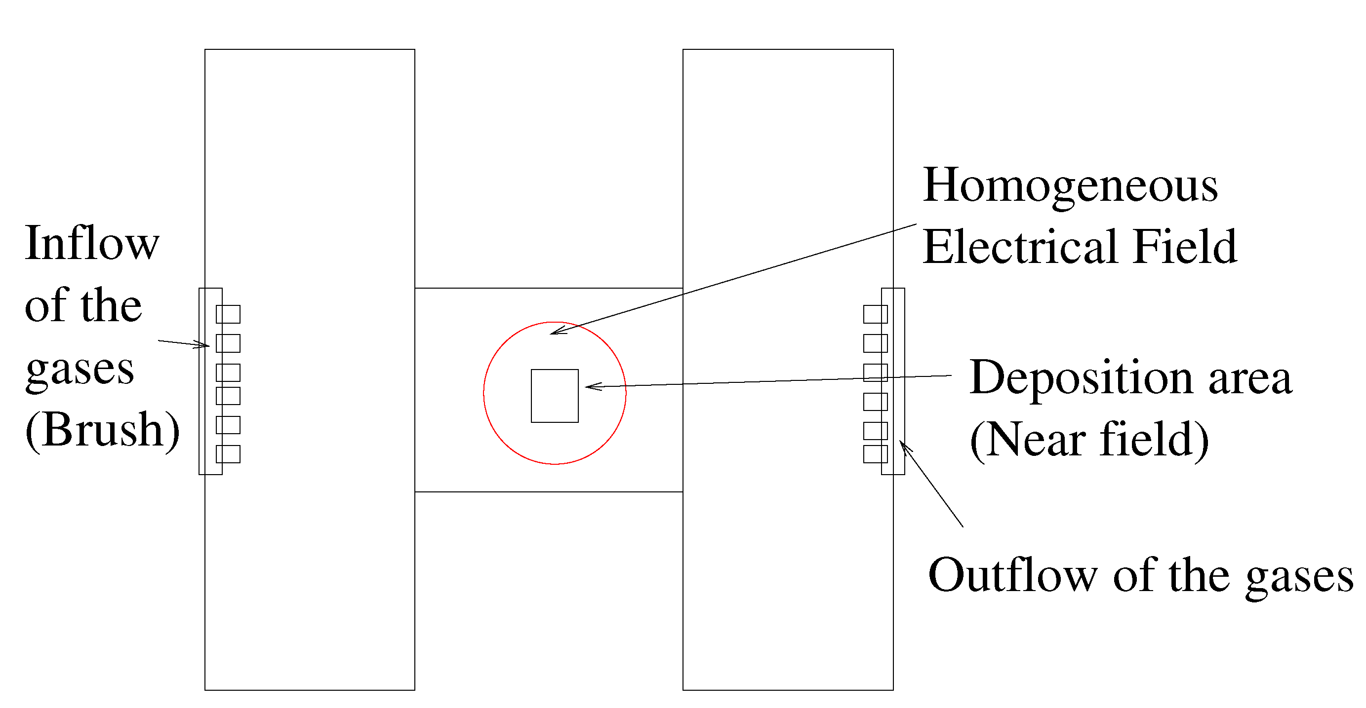
In
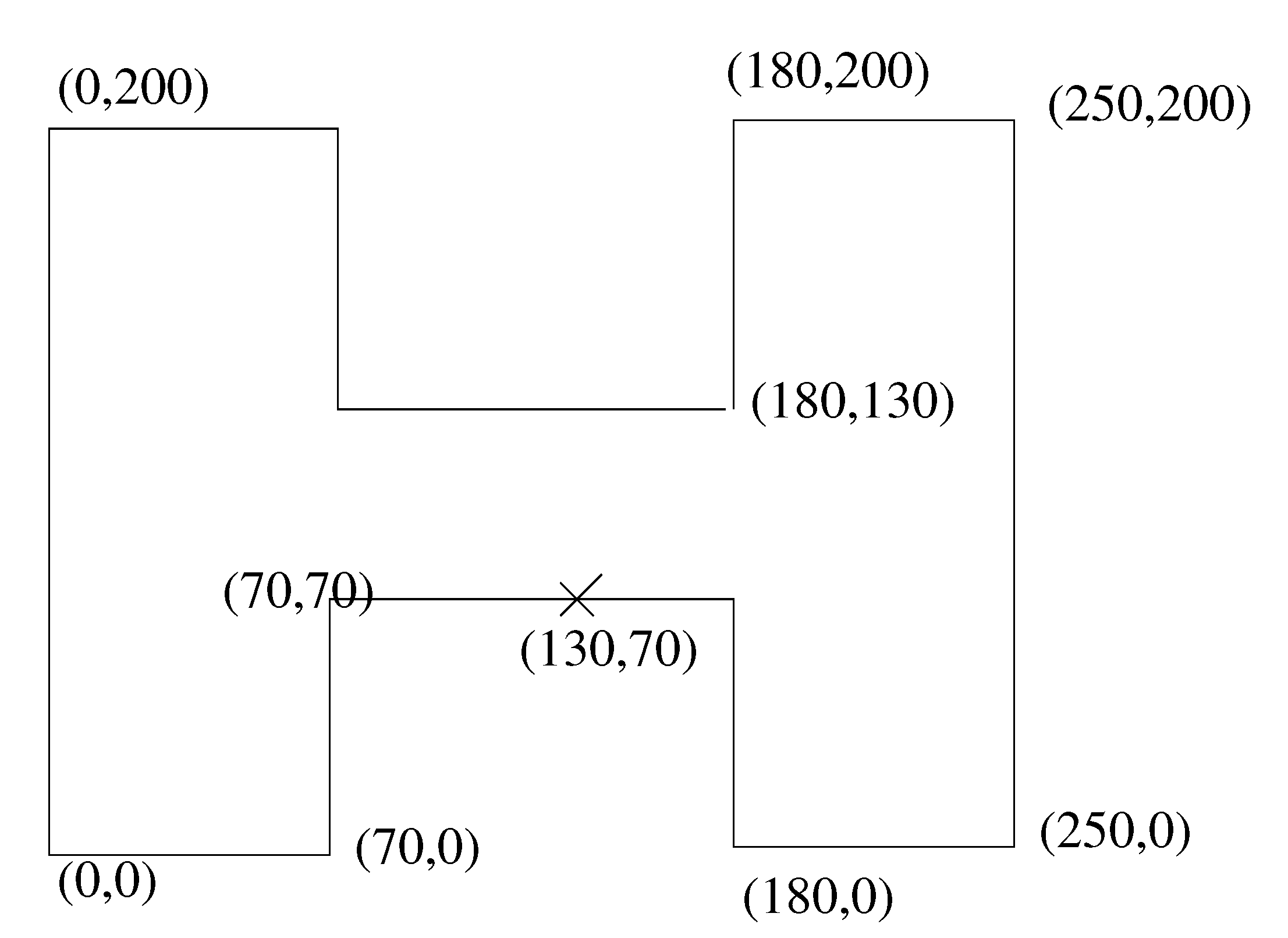
Figure 6, the underlying geometry of the apparatus is shown. The inflow of the precursor gases are at the left and right of the top of the apparatus, while the outflows are at the left and right bottom. The measured point
is in the middle of the deposition area at which the deposition rates could be measured.
Figure 6.
The geometry of the apparatus with the measurement points (we apply as unit in the geometry).
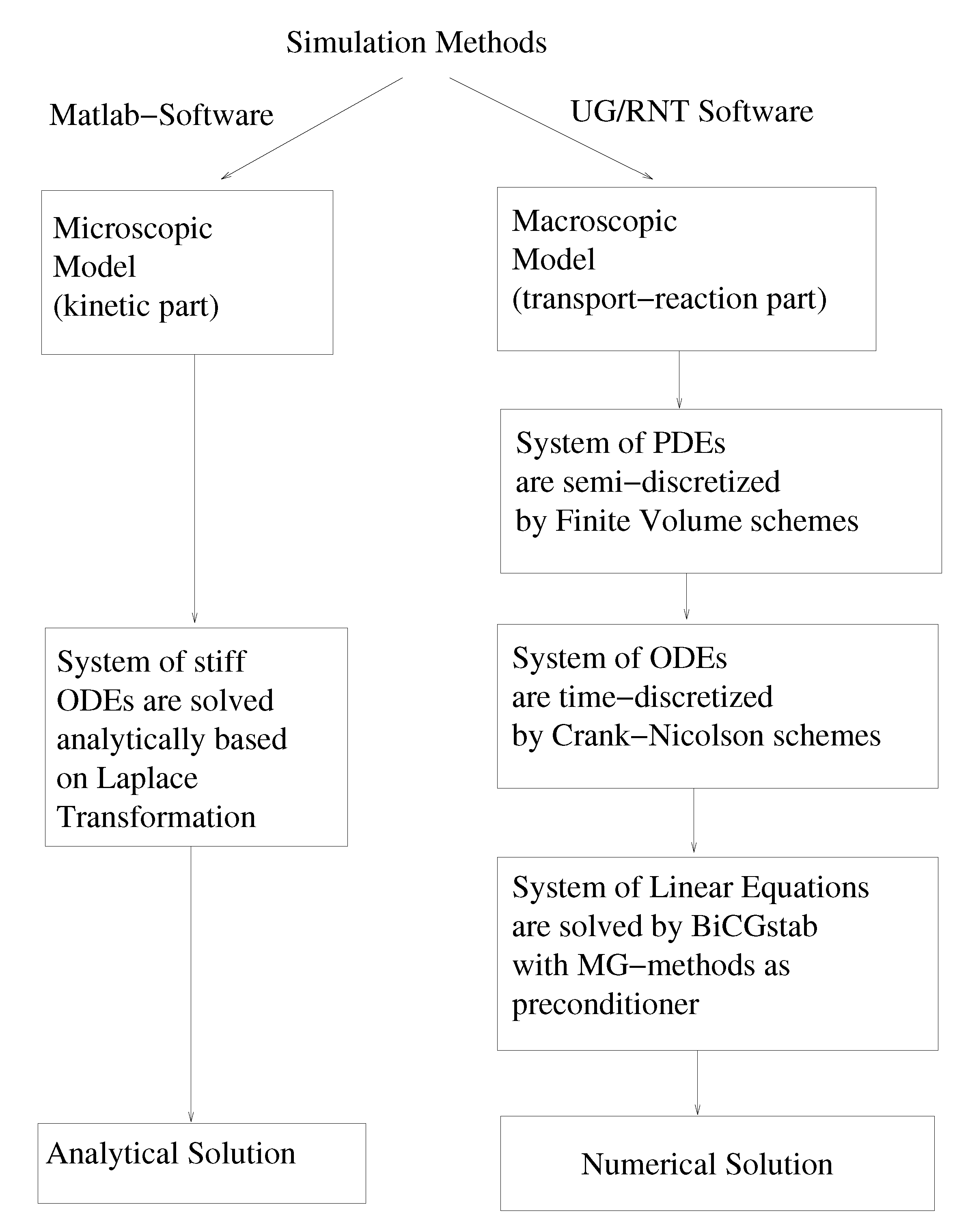
4.2.1. Parameters of the Model Equations
In the following, all the parameters of the model equation (2) are given in
Table 2. Here, we have the physical experiments and approximate to the temperature parameters of
T = 400, 600, 800 K. For the physical experiment, we have the following parameters (see
Table 3).
Table 2.
Model Parameters.
Table 2.
Model Parameters.
| density | |
| mobile porosity | |
| diffusion | |
| longitudinal dispersion | |
| transversal dispersion | |
| retardation factor | (Henry rate) |
| velocity field | |
| decay rate of the species of 1st EX | |
| decay rate of the species of 2nd EX | , |
| decay rate of the species of 3rd EX | , |
| Geometry (2d domain) | . |
| Boundary | Neumann boundary at |
| top, left and right boundaries. |
| outflow boundary |
| at the bottom boundary |
Table 3.
Approximated deposition rates and comparison to physical experiments.
Table 3.
Approximated deposition rates and comparison to physical experiments.
| W | T | | | | Physical ratio (Si:C) | Numerical ratio (Si:C) |
|---|
| 100 | 700 | | | | 0.569 | 0.568 |
| 300 | 700 | | | | 0.744 | 0.740 |
| 900 | 700 | | | | 0.919 | 0.9 |
| 100 | 400 | | | | 0.617 | 0.6103 |
| 500 | 400 | | | | 0.757 | 0.745 |
| 500 | 400 | | | | 0.704 | 0.691 |
| 900 | 400 | | | | 1.010 | 1.017 |
| 900 | 400 | | | | 1.0 | 1.0 |
| 100 | 400 | | | | 0.342 | 0.342 |
The discretization and solver method are the following:
For the spatial discretization method, we apply finite volume methods of the second order with the parameters in
Table 4.
For the time discretization method, we used the CrankNicolson method (second order) with the parameters in
Table 5.
The discretized equations are solved with the following methods, see the description in
Table 6.
The initialization of sources of the equations are solved with the following parameters in
Table 7.
Table 4.
Spatial discretization parameters.
Table 4.
Spatial discretization parameters.
| spatial step size | |
| refined levels | 6 |
| limiter | slope limiter |
| test functions | linear test function |
| reconstructed with neighbor gradients |
Table 5.
Time discretization parameters.
Table 5.
Time discretization parameters.
| Initial time-step | |
| controlled time-step | |
| Number of time-steps | |
| Time-step control | time steps are controlled with |
| the Courant number |
Table 6.
Solver methods and their parameters.
Table 6.
Solver methods and their parameters.
| Solver | BiCGstab (Bi-conjugate gradient method) |
| Preconditioner | geometric multigrid method |
| Smoother | GaussSeidel method as smoothers for |
| the multigrid method |
| Basic level | 0 |
| Initial grid | uniform grid with 2 elements |
| Maximum Level | 6 |
| Finest grid | uniform grid with 8192 elements |
Table 7.
Parameters of the source concentration.
Table 7.
Parameters of the source concentration.
| 81 point sources of SiC at the position | |
| Line source of H at the position | |
| Amount of the permanent source concentration | = 0.4, 0.7, 0.8, 0.85, 0.84, 0.82, 0.8, |
| 0.6, 0.4, 0.2, 0.0., |
| Number of time steps | 200 |
4.2.2. Numerical Results of the Model Equations
The numerical experiments now to be discussed are approximations to the SiC experiments. The underlying software tool is
, which was developed to solve discretized partial differential equations (see [
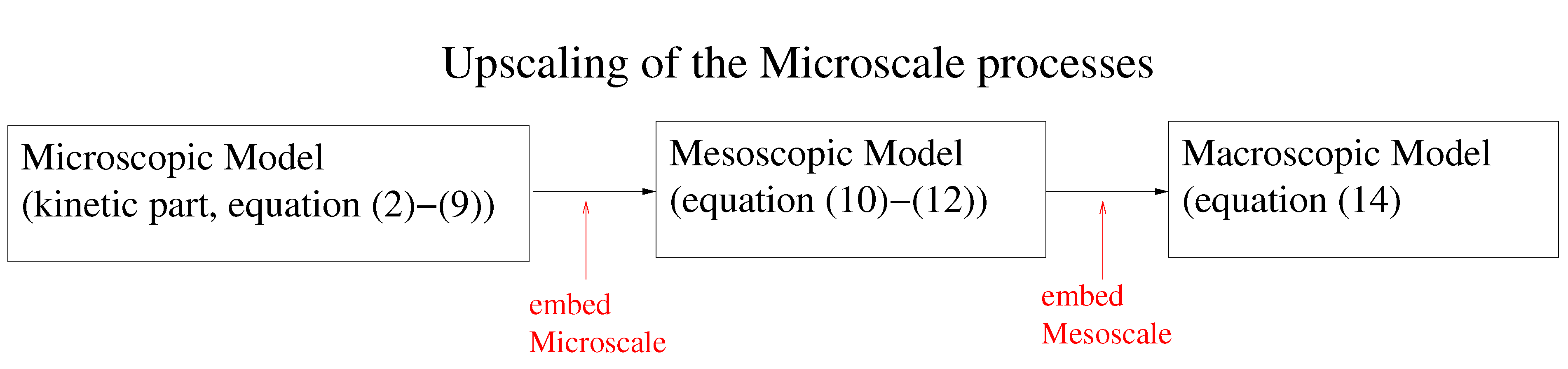
4]). We use the tool to solve transportreaction equations. For the SiC, we obtain a different setup for the physical experiment, including the Bias voltage of the electric field, which is simulated as a retardation to the species. For the multiscale reaction equations, we can simplify the reaction process with respect to the slow scales. We consider an upscaled kinetic process, given by:
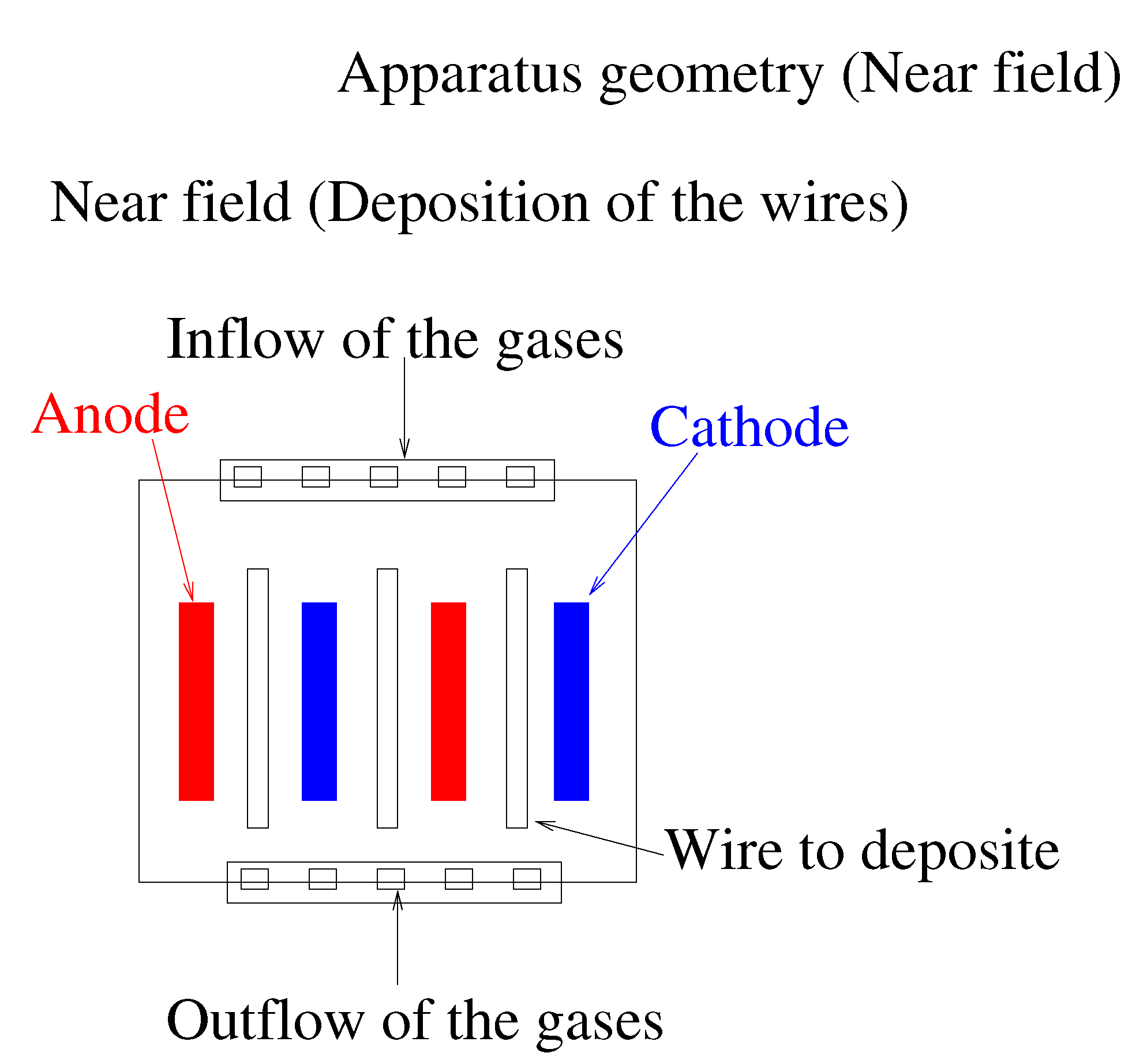
In the following numerical experiment, we concentrate on the near-field computations of the deposition area (see
Figure 2). We apply the transport-reaction parts (see Equation (
1)) and the upscaled reaction (see Equation (45)).
We deal with the following parameters. Here we assume a constant velocity field and start with the species
and H, which are given as point and line sources (see
Table 8). We add some more H concentration to stabilize the scheme. We take here the concentration of
as a point source, and the concentration of H is a line source. Further, we are interested in the relation between SiC and Si concentrations at the end of the deposition process. In
Figure 7 and
Figure 8, we present the concentration SiC, Si and
after 100 and 200 time-steps. In the initialization, the amount of the
and Si species is not balanced; also, the amount of the
species are too high. In such a situation, we would have a wrong deposition rate. In the later situation (see
Figure 8), after 200 time steps, we see that the situation is balanced with respect to the SiC and Si concentrations. Here, fast reactions of
and H have been passed, and we only have smooth transportreaction process. Now, the deposition of the layer is homogeneous and our rate is nearly
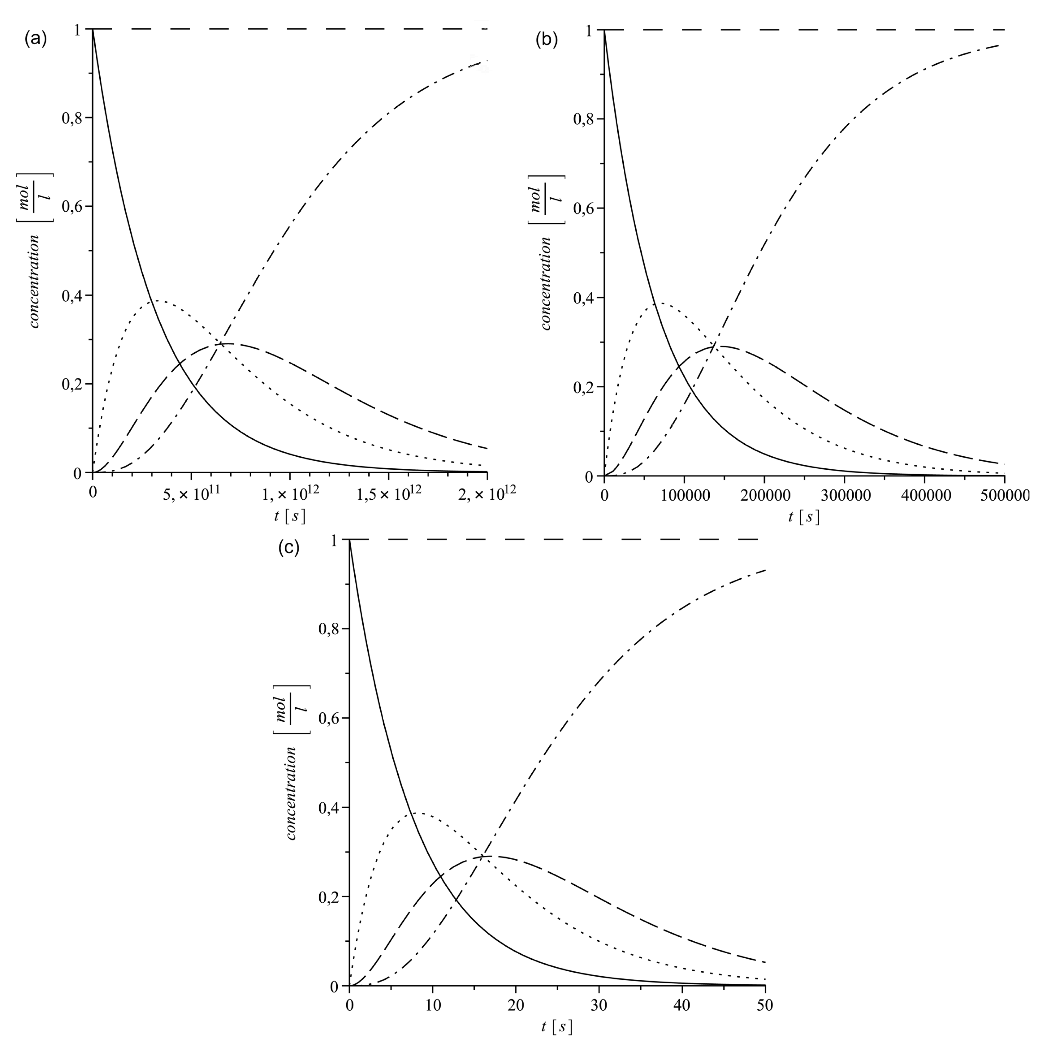
. In
Figure 9, we show the results after the long deposition period of 200 time-steps. Here, the deposition rates are done with a 81 point sources experiment. Such a large amount of sources helps to homogenize the deposition in a large deposition region. We see a nearly constant deposition of the species SiC, while we dust small concentrations to the deposition area.
Table 8.
Rate of the concentration.
Table 8.
Rate of the concentration.
| Rate at the end of the deposition at the deposited layer: |
|---|
|
|
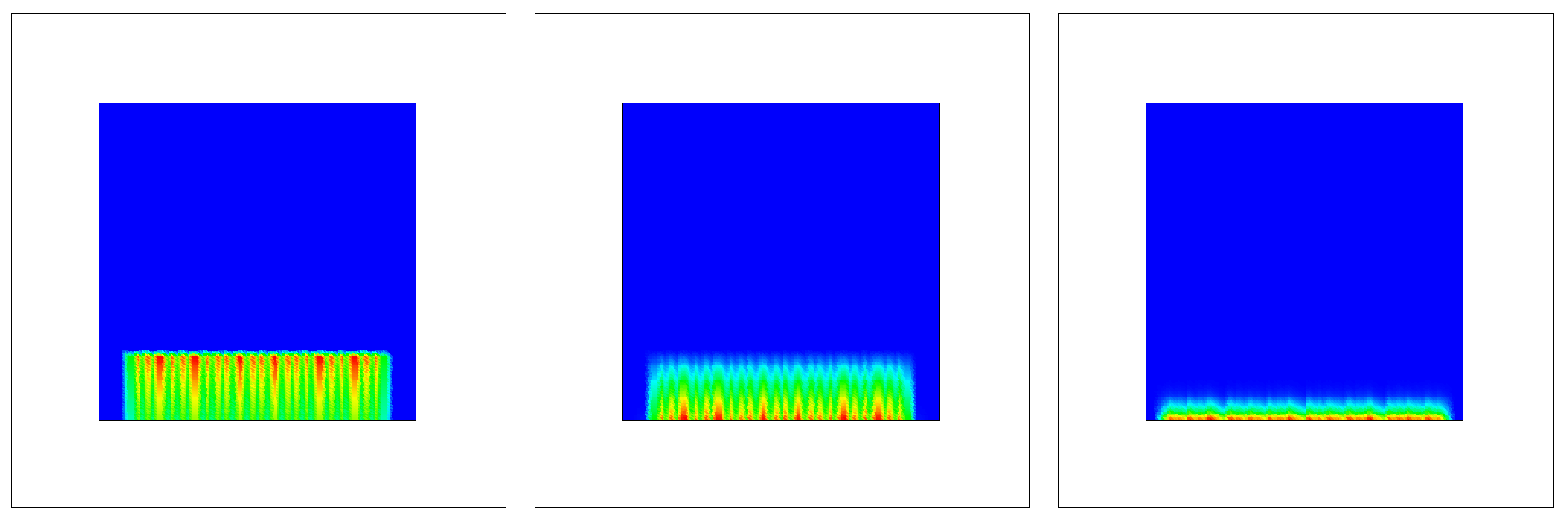
Figure 7.
Experiment with moving point sources: SiC experiment after 100 time-steps, where a high concentration is red, a low concentration is blue (left figure: SiC concentration; middle figure: Si concentration; right figure: H concentration).
Figure 7.
Experiment with moving point sources: SiC experiment after 100 time-steps, where a high concentration is red, a low concentration is blue (left figure: SiC concentration; middle figure: Si concentration; right figure: H concentration).
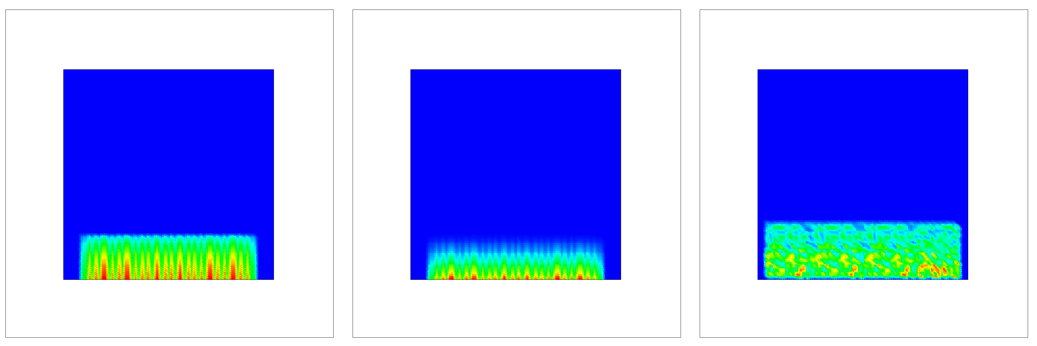
Figure 8.
Experiment with moving point sources: SiC experiment after 200 time-steps, where a high concentration is red, a low concentration is blue (left figure: SiC concentration; middle figure: Si concentration; right figure: H concentration).
Figure 8.
Experiment with moving point sources: SiC experiment after 200 time-steps, where a high concentration is red, a low concentration is blue (left figure: SiC concentration; middle figure: Si concentration; right figure: H concentration).
Figure 9.
Deposition rates for the 81 point sources experiment (x-axis: time in s, y-axis: concentration in ).
Figure 9.
Deposition rates for the 81 point sources experiment (x-axis: time in s, y-axis: concentration in ).
Remark 2 The numerical experiments in the near-field can be approximations of the real-life physical experiments. Both experiments show the influence of temperature, while for low temperatures, we can assume we are dealing with slow time-scale reaction equations. In such regimes, we obtain the best results with multiple sources and long-time depositions. We apply further different experimental situations, and the best deposition result is obtained with low temperature and high power assumptions. At least homogeneous concentrations below the deposition area can be achieved with a large amount of sources. The near-field simulations obtain an optimum at the low temperature of 400 °C and a high plasma power of about 900 W. Such results are also obtained in our physical studies (see [
27]).


