
Kinetics of Micellization and Liquid–Liquid Phase Separation in Dilute Block Copolymer Solutions

Osaka Study Center, The Open University of Japan, 4-9-23, Onohara-Higashi, Osaka 562-0031, Japan
Polymers 2023, 15(3), 708; https://doi.org/10.3390/polym15030708
Submission received: 30 December 2022
/
Revised: 22 January 2023
/
Accepted: 24 January 2023
/
Published: 31 January 2023
(This article belongs to the Special Issue State-of-the-Art Polymer Science and Technology in Japan (2021,2022))
Abstract
:A lattice theory for block copolymer solutions near the boundary between the micellization and liquid–liquid phase separation regions proposes a new kinetic process of micellization where small concentrated-phase droplets are first formed and then transformed into micelles in the early stage of micellization. Moreover, the thermodynamically stable concentrated phase formed from metastable micelles by a unique ripening process in the late stage of phase separation, where the growing concentrated-phase droplet size is proportional to the square root of the time.

1. Introduction
An amphiphilic diblock copolymer forms a micelle in a selective solvent. If the block copolymer is thermosensitive, pH-sensitive, or ionic strength-sensitive, the kinetics of the micelle formation in dilute homogeneous block copolymer solutions can be studied experimentally by temperature-jump, pH-jump, or salt-jump experiments. Such kinetic studies have been carried out extensively for various block copolymer solutions thus far [1,2,3,4,5,6,7,8,9,10,11,12,13,14,15,16]. The micellization process of block copolymers is much slower than that of small molecular surfactants, so the former kinetics is easier than the latter, but the micellization of the block copolymers is still fast to study experimentally.
The micellization kinetics of both block copolymers and small molecular surfactants have been analyzed on the basis of the stepwise aggregation mechanism of monomers [17,18,19,20,21]. This mechanism was first proposed by Aniansson and Wall in 1974 [17] to explain the micellization kinetics of small molecular surfactants, which resembles the kinetic theory of nucleation (the formation of a new phase within a metastable phase) [19,21], and was also utilized to analyze block copolymer micellization kinetics [3,4,5,6].
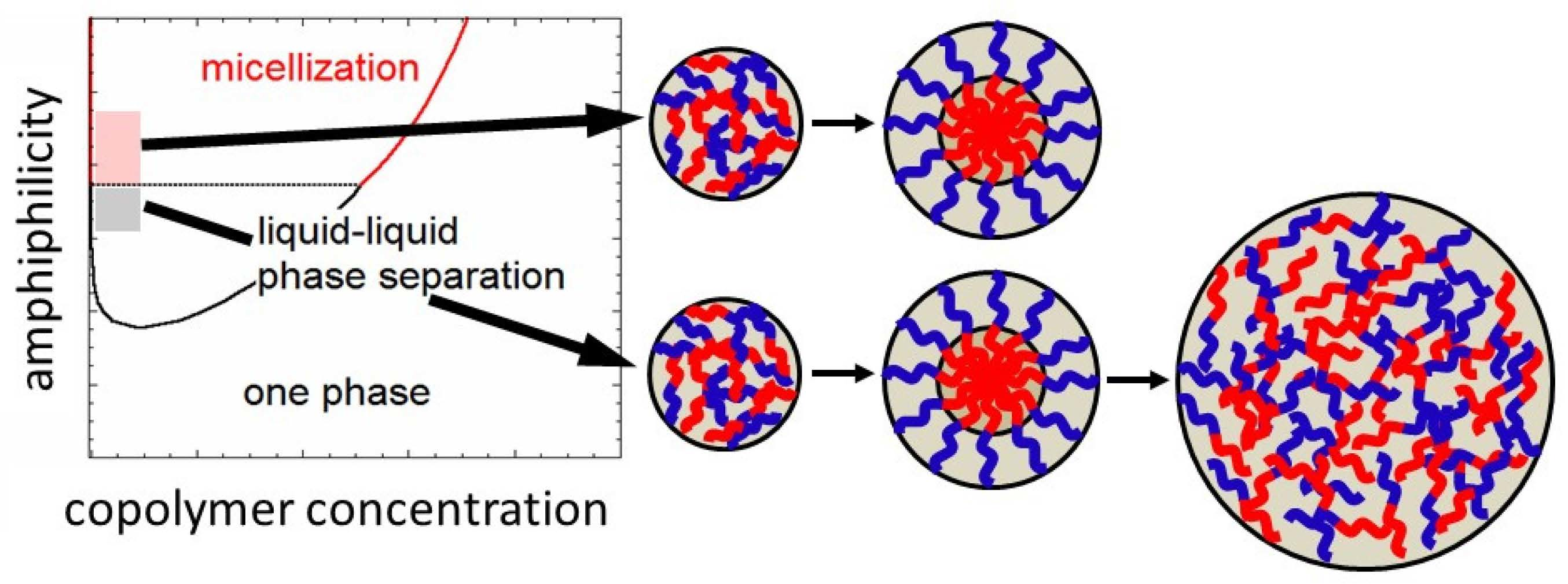
More recently, our group investigated the self-assemblies of several thermosensitive and ionic strength-sensitive block copolymers in dilute aqueous solutions, and found the competition between the micellization and liquid–liquid phase separation of those block copolymers [22,23,24,25,26]. The competition comes from weaker amphiphilicity of the block copolymers, which was explained semi-quantitatively by the lattice theory [27]. Furthermore, the lattice theory predicted that micellization prefers to liquid–liquid phase separation at a lower hydrophobic content of the copolymers, and the prediction was demonstrated experimentally using a thermosensitive block copolymer in aqueous solutions [26].
The present study deals with the kinetics of the micellization as well as of the liquid–liquid phase separation in dilute block copolymer solutions, where the micellization competes with the liquid–liquid phase separation. The liquid–liquid phase separation starts from the formation of small concentrated-phase droplets, which are thermodynamically less stable than the macroscopic concentrated phase due to the extra interfacial Gibbs energy. The preference of concentrated-phase droplets and micelles may be reversed during the growing process of micellization or phase separation. The judgement of the preference needs to quantitatively compare the Gibbs energy of formation of the concentrated-phase droplet with that of the micelle. Such a comparison proposes the unique kinetics of micellization and concentrated-phase droplet growth in the early and late stage, respectively, as explained in what follows.
2. Thermodynamics
2.1. Models and Mixing Gibbs Energy Densities [27]
Let us consider an aqueous solution of a block copolymer that consists of a hydrophilic A-chain of the degree of polymerization PA and a hydrophobic B-chain of the degree of polymerization PB. The hydrophilic and hydrophobic contents of the copolymer are given by xA = PA/(PA + PB) and xB = PB/(PA + PB), respectively. The monomer units of the A- and B-chains as well as the solvent water molecule are assumed to possess the same size a (the unit lattice size).
Figure 1a shows a schematic illustration of the spherical micelle. We assumed that both the hydrophobic core and hydrophilic shell regions of the micelle were uniform, and that the A- and B-block chains were completely excluded from the core and shell regions of the micelle, respectively, as shown in Figure 1, to calculate the thermodynamic quantities of the micellar phase. In this theory, the micelle is regarded as a thermodynamic phase. This simplified model of the spherical micelle resembles that used by Leibler et al. [28], although in the present model, the radii of the core Rcore and of the whole micelle Rm are given by
Here, the exponent α was assumed to be 0.5 for the Gaussian chain in this paper, but this α value does not essentially change the following semi-quantitative argument. Leibler et al. [28] considered a homopolymer as the solvent, and treated Rcore and Rm as variables, determined from the free energy minimization condition.
The average volume fraction of the copolymer ϕP in the micellar phase is given by ϕP = 3(PA + PB)m/(4πRm3), where m is the aggregation number of copolymer chains in the spherical micelle. The volume fractions of the A- and B-block chains in the shell and core regions (ϕA,s and ϕB,c), respectively, can be calculated from ϕP by
By extending the Flory–Huggins theory [29], we can formulate the mixing Gibbs energy density (per the unit lattice site) ∆gm(ϕP) in the micellar phase as [27]
where kBT is the Boltzmann constant multiplied by the absolute temperature, and κ is a constant defined by
χAS, χBS, and χAB are the interaction parameters between the A-chain and the solvent, between the B-chain and the solvent, and between the A- and B-chains, respectively, and γc is the interfacial tension between the core and shell regions. Using the theory of Noolandi and Hong [30], as explained in Appendix A, the expression of γc as well as the thicknesses of the corresponding interfaces dI,c are given by
where ∆fc(0) is defined as
with ϕS,s = 1 − ϕA,s and ϕS,c = 1 − ϕB,s. Although not shown in Figure 1a, the interfacial region of the micelle has a sharp concentration gradient, as illustrated in Figure A1 in Appendix A. In Equation (3), the term of the interfacial tension between the shell region of the micelle and the coexisting dilute phase was neglected, because ϕA,s and χAS were considerably smaller than ϕP,d and (cf. Equation (8)), respectively.
Figure 1b illustrates the schematic diagram of the spherical concentrated-phase droplet, where both volume fractions of the A- and B-chains are uniform. Through a simple extension of the Flory–Huggins theory [29], the mixing Gibbs energy density ∆gd(ϕP) in the concentrated-phase droplet is written as
where ϕP and ϕS = 1 − ϕP are the volume fractions of the copolymer and the solvent in the droplet phase, respectively, and is the average interaction parameter defined by
and γd is the interfacial tension between the concentrated-phase droplet and the homogeneous (dilute) solution phase. Not illustrated in Figure 1b, the interfacial region of the droplet must possess a sharp concentration gradient. There are two limiting cases: one is that only A-block chains make contact with the coexisting dilute phase at the interface, like the micelle, and the other is to assume that the composition ϕA(x)/ϕB(x) (cf. Figure A1 in Appendix A) is uniform, even at the interface. Here, we took the latter limiting case (i.e., the total copolymer volume fraction ϕP(x) changes under the constant composition). Then, the expression of γd and the thickness of this interface dI,d are obtained from Equations (A4)–(A6) in Appendix A by
with the copolymer volume fraction ϕP,h(Rd) in the dilute solution phase coexisting with the concentrated-phase droplet of the radius Rd and
[ϕS = 1 − ϕP and ϕS,h(Rd) = 1 − ϕP,h(Rd)].
The excess chemical potentials (per molecule) of the solvent ∆μS,d and of the copolymer ∆μP,d in the droplet phase can be calculated from Equation (7) as
Finally, the mixing Gibbs energy density ∆gh(ϕP) as well as the excess chemical potentials of the solvent ∆μS,h and of the copolymer ∆μP,h in the homogeneous copolymer solution phase are given by [29]
which correspond to Equations (7) and (11) in the limit of infinite Rd.
2.2. Phase Diagram
When is sufficiently large, concentrated-phase droplets with the copolymer volume fraction ϕP,d(Rd) appear in the homogeneous copolymer solution, and if the amphiphilicity is strong enough (or χBS >> χAS), the micellar phase with the copolymer volume fraction ϕP,m is formed in the homogeneous copolymer solution. The copolymer volume fractions ϕP,d(Rd) and ϕP,m can be calculated from the following phase equilibrium conditions
where ∆μS,I and ∆μP,i (i = h, d, m) are the excess chemical potentials (per molecule) of the solvent and of the copolymer, respectively, in the homogeneous solution (i = h), in the droplet phase (i = d), and in the micellar phase (i = m); ϕP,h(Rd) and ϕP,h(m) are the copolymer volume fractions of the homogeneous (dilute) phase coexisting with the droplet and micellar phases, respectively.
As a case study, Figure 2 shows three mixing Gibbs energy densities, ∆gh, ∆gd, and ∆gm as functions of ϕP for an AB diblock copolymer solution with PA = PB = 100 (xA = xB = 0.5), χAS = 0.4, χAB = 0, and χBS = 1.122. The blue curve (∆gd) for the droplet phase shifts slightly upward from the black curve (∆gh) for the homogeneous solution due to the interfacial tension term in Equation (7). The red curve (∆gm) for the micellar phase has stronger curvature than the black and blue curves. By choosing χBS = 1.122, we can draw a common tangent to the black and red curves (although not clearly shown, the black curve was convex downward at ϕP~0), which makes contact with the black and red curves at ϕP,h(∞) (=ϕP,h(m)), ϕP,m, and ϕP,d(∞). When χBS < 1.122, the red curve shifts upward, and when χBS > 1.122, the red curve shifts downward relative to the black curve, indicating that the homogeneous solution and the micellar phase are thermodynamically stabler at lower and higher χBS, respectively [27].
From the Gibbs–Duhem relation, the mixing Gibbs energy density is related to the excess chemical potential by
and this equation verifies that ϕP,h(m) and ϕP,m in Figure 2 fulfill the phase equilibrium conditions given by Equation (13b). On the other hand, the Gibbs–Duhem relation does not hold for the droplet phase due to the interfacial tension term in Equation (7), which is not proportional to the total number of molecules in the system. However, the coexisting phase volume fractions ϕP,d(Rd) and ϕP,h(Rd) can be calculated by solving the simultaneous Equation (13a).
Pairs of the coexisting phase volume fractions, ϕP,h(∞) and ϕP,d(∞), ϕP,d(Rd) and ϕP,h(Rd), and ϕP,h(m) and ϕP,m, are obtained as functions of χBS, at constant χAS = 0.4 and χAB = 0 [and at Rd/a = 20 for the pair of ϕP,d(Rd) and ϕP,h(Rd)]. Figure 3 shows the phase diagram under this condition. Here, the black, blue, and red curves indicate coexisting homogeneous, droplet, and micellar phases, respectively, and solid and broken curves the stable and unstable (or metastable) states, respectively. The small black circle in the figure indicates the critical point for the liquid–liquid phase separation. It was noted that there is no critical point for the homogeneous-droplet phase equilibrium. For the coexistence of the micellar and homogeneous phases, we can draw two common tangents (the two tangents become identical at χBS = 1.122 in Figure 2), and the phase diagram has two coexistence regions of the micelle + dilute phase and micelle + concentrated phase, as shown in Figure 3. In what follows, we focused only on micellization and the concentrated-phase droplet formation in dilute copolymer solutions.
The micellar phase formation thermodynamically prefers the formation of the droplet phase with Rd/a = 20 at χBS > 1.048, as indicated by the blue thin dotted line in Figure 3. This phase boundary shifts to lower χBS than the boundary between the micellization and macroscopic liquid–liquid phase separation (cf. the red thin dotted line in Figure 3), because the interfacial tension term in ∆gd(ϕP) given by Equation (7) destabilizes the droplet concentrated phase. With increasing Rd, the boundary between the micelle and droplet phases approaches the red thin dotted line, located at χBS = 1.122.
As already shown in a previous work [27], when χAS decreases, the biphasic region of the liquid–liquid phase separation goes up (Figure 3), while the binodal curves for the micelle–homogeneous phase equilibrium do not change as much. Thus, the stable liquid–liquid phase separation region becomes narrower and finally disappears in the phase diagram. A similar change in the phase diagram occurs when χAB increases.
In Figure 3, the black thin dot-dash curve indicates the spinodal, calculated by [29]
within the spinodal region, the homogeneous phase is not stable with respect to long-ranged concentration fluctuation induced by thermal agitation, and the spinodal decomposition can take place in the early stage of the liquid–liquid phase separation. On the other hand, the concentration fluctuation is unstable in the homogeneous solution, outside the spinodal region. Thus, when the homogeneous solution is jumped into the region between the spinodal and binodal curves in the dilute region, the concentrated-phase droplet and spherical micelle may be formed in the solution through the nucleation–growth mechanism.
3. Kinetics of Micellization and Liquid–Liquid Phase Separation
3.1. Growth of the Concentrated-Phase Droplet and Spherical Micelle in the Early Stage
Let us consider a metastable dilute homogeneous solution with a copolymer volume fraction ϕP,h between ϕP,h(Rd) and the lower spinodal volume fraction ϕP,sp− (cf. Equation (15)). When a spherical concentrated-phase droplet with the radius Rd and the copolymer volume fraction ϕP,d is formed in this homogeneous copolymer solution, the Gibbs energy of the droplet formation δGd is given by
where ϕP,d is assumed to be equal to the equilibrium copolymer volume fraction ϕP,d(Rd) calculated by the phase equilibrium condition, Equations (13a) and (13b), as a function of the droplet radius Rd, and the aggregation number m is calculated by
Because the droplet of the radius Rd is in equilibrium with the homogeneous solution with ϕP,h(Rd) (<ϕP,h), there was a concentration gradient in the vicinity of the droplet surface and the droplet grew through the diffusion flow of the copolymer from the homogeneous solution.
Similarly, when a spherical micelle with the aggregation number m and the copolymer volume fraction ϕP,m formed in the dilute homogeneous copolymer solution with the copolymer volume fraction ϕP,h (ϕP,h(m) < ϕP,h < ϕP,sp−), the Gibbs energy of the micelle formation δGm is given by
where ϕP,m is calculated from m by
where Rm is calculated by Equation (1).
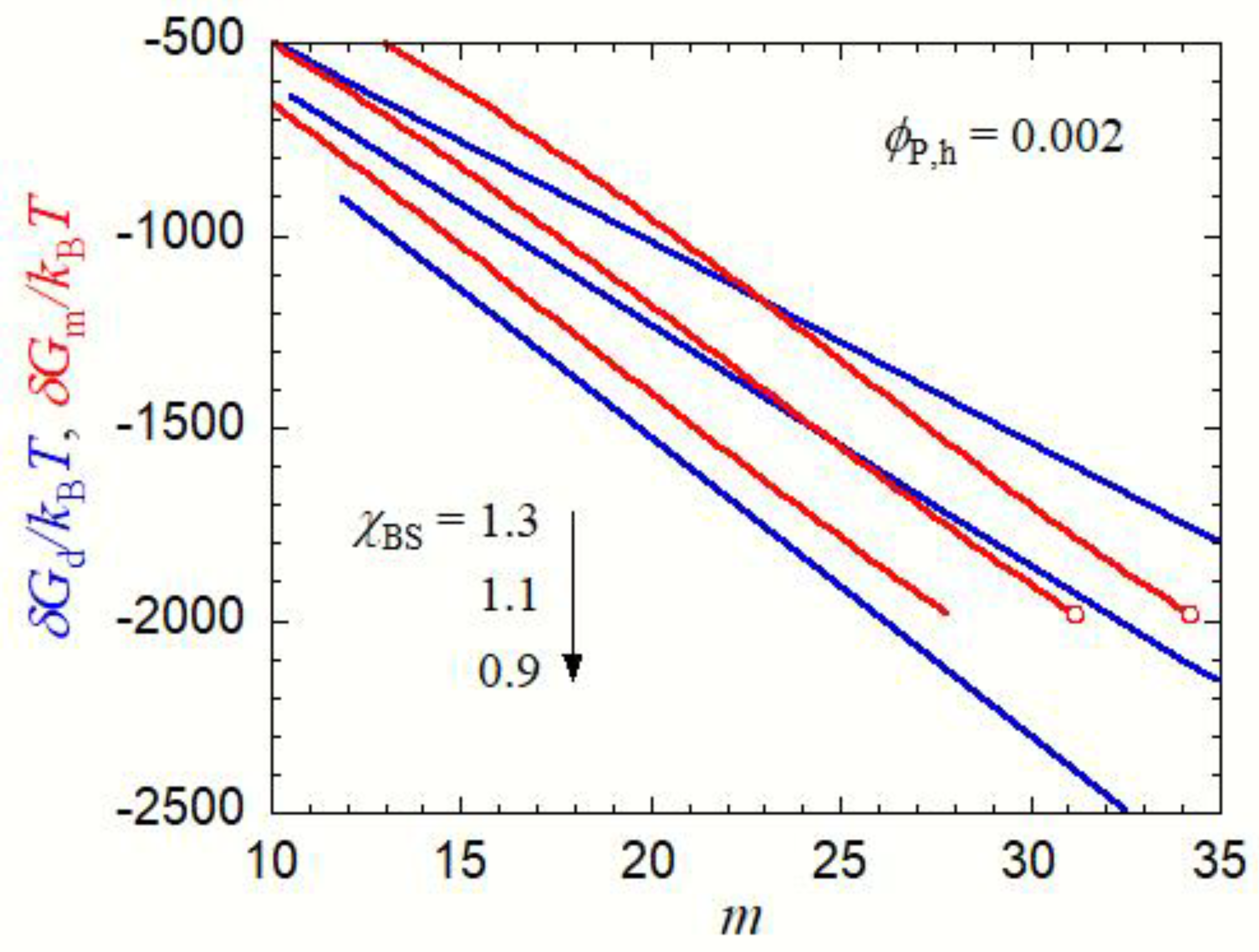
In Figure 4, δGd and δGm are plotted against the aggregation number m in the copolymer solution at ϕP,h = 0.002. As seen in Figure 3, micellization is preferred to the liquid–liquid phase separation at χBS = 1.3, but δGm for the micelle is higher than δGd for the concentrated-phase droplet at m < 23. Thus, if χBS abruptly changes from a low value (<0.85, the one-phase condition) to 1.3, small concentrated-phase droplets form more easily than the micelles with the same m (<23) in the copolymer solution. However, when these concentrated-phase droplets grow, they become less stable than the micelle at m > 23. This indicates that the core–shell structure may be developed inside the growing droplets. Finally, the micelles with m = 34 (the red circle in Figure 4 for χBS = 1.3) form in the copolymer solution in the equilibrium state.
A similar relation between δGd and δGm also holds at χBS = 1.1. Concentrated-phase droplets first form in the copolymer solution, and they may be transformed into micelles with m = 31 (the red circle in Figure 4 for χBS = 1.1) during the growing process. Although the liquid–liquid phase separation is preferred to the micellization at χBS = 1.1 in the final equilibrium state, as seen in Figure 3, the micelle is a metastable state, and the formation of the concentrated phase of a large size must overcome the activation Gibbs energy barrier. The late stage of the concentrated-phase droplet growth in such a solution is discussed in the next Section 3.2.
At χBS = 0.9, δGd is smaller than δGm in the whole m range, and the concentrated-phase droplet keeps growing without transforming into the micelle. In the equilibrium state, the liquid–liquid phase separation is preferred to micellization (cf. Figure 3).
The kinetics of liquid–liquid phase separation and micellization in the early stage has been argued in the scenario of the nucleation–growth mechanism thus far. That is, the nuclei of the concentrated phase and the micelle are formed step-wise from the unimer (m = 1) [17,18,19,20,21]. In the concentrated-phase droplet, the copolymer chain was assumed to take the random coil conformation, and the concentration gradient near the droplet surface was neglected to derive Equation (7). Thus, Equation (7) for ∆gd(ϕP) holds only at Rd larger than <R2>1/2/2 + dI,d, where <R2>1/2 is the mean-square end-to-end distance of the copolymer chain [=(PA + PB)a2], and dI,d is calculated by Equation (9). In Figure 4, m = 10 is close to the lower limit where Equation (7) holds. Moreover, in the micelle model used in this work, Rm and Rcore are given by Equation (1), which may hold only when ϕB,c is sufficiently high. For small m, where ϕB,c is low, B-block chains forming the core may shrink to escape contact with the solvent, so our micelle model cannot be used for such a small m. Under the condition of Figure 4, ϕB,c ≈ 0.25 at m = 10, and our micelle model may not be applied at m considerably smaller than 10. Therefore, Equations (16) and (18) cannot be used to discuss the nucleation processes of liquid–liquid phase separation and micellization [21].
Although these nucleation processes were not discussed, the above argument proposes a new kinetics of the micellization process in the early stage (i.e., the transformation from the small concentrated-phase droplet to the spherical micelle). As above-mentioned, the stable liquid–liquid phase separation region becomes narrower and finally disappears in the phase diagram, when χAS decreases and/or χAB increases. Nevertheless, the same kinetics of the micellization process in the early stage can also be expected at lower χAS and higher χAB, because δGd < δGm at small m, even if the liquid–liquid phase separation region becomes unstable, as demonstrated in Figure 4 at χBS = 1.3.
3.2. Modification of the Lifshitz–Slyosov Theory in the Late Stage of the Phase Separation
As above-mentioned, the micellar phase is the metastable state at χBS = 1.1 (more generally at χBS from 1.03 to 1.122) within the biphasic region in Figure 3, and the thermodynamically equilibrium state is the liquid–liquid phase separation (where the concentrated-phase droplet size is macroscopic) in that region in Figure 3. The phase boundary (the blue horizontal dotted line in Figure 3 at Rd/a = 20) shifts to χBS = 1.1 at Rd/a = 50, so the concentrated-phase droplet with Rd/a > 50 is stabler than the micelle. If the concentrated-phase droplet of such a large size is formed occasionally by overcoming the activation Gibbs energy barrier, it keeps growing without developing the micellar structure. Since ϕP,h(Rd) < ϕP,h(m) at Rd/a > 50, the growth of such large droplets in the solution is accompanied by the dissociation of micelles existing in the solution. This droplet ripening process in the micellar solution is different from the conventional Ostwald ripening in the usual liquid–liquid phase separation of the late stage.
The conventional Ostwald ripening process is quantitatively dealt with by the Lifshitz–Slyozov theory [31,32]. In the theory, the droplet with the radius Rd is in equilibrium with the homogeneous dilute solution (the mother solution) with the concentration ϕP,h(Rd) given by (in terms of our notations)
where σ is a constant parameter proportional to the interfacial tension. When the average concentration of the mother solution is denoted as , larger droplets with ϕP,h(Rd) < can grow, while smaller droplets with ϕP,h(Rd) > dissociate along with diffusing the solute into the mother solution. The critical radius R* for the growing droplet is given by
Along with the droplet growth, the concentration of the mother solution is reduced, and R* increases with time t. Although the σ calculated from the results of ϕP,h(Rd) obtained by Equations (13a) and (13b) was slightly dependent on Rd, we neglected this dependence according to Lifshitz and Slyozov in what follows, of which the approximation is good only at sufficiently large Rd, or in the late stage of the phase separation
The concentration of the mother solution containing spherical micelles should maintain the critical micelle concentration ϕP,h(m), even during the growth of concentrated-phase droplets. Thus, Equation (21) should be replaced by
Thus, R* is independent of t until all micelles disappear in the solution, which is in contrast with the Lifshitz–Slyozov theory, and the theory should be modified as follows.
New parameters u and tr are defined by
where D is the diffusion coefficient of the solute in the mother solution. Using these parameters, the droplet growth rate du/dtr can be written as
By integrating this equation, we obtain
with the integration constant C0. Figure 5 shows the time dependence of Rd for the growing droplet (Rd = R* at t = 0) in the micellar solution, calculated by Equation (25). When u and tr are sufficiently large, Equation (25) can be approximated to
This is in contrast with the Lifshitz–Slyozov theory, where the average radius of the droplet is proportional to t1/3 in the late stage [31,32]. After all micelles disappear in the solution, the droplet growth should obey the Ostwald ripening (i.e., larger droplets grow by consuming the solute provided by dissociating smaller droplets). As the result, the average radius of the growing droplet is proportional to t1/3.
4. Concluding Remarks
A discussion has been made on the phase separation kinetics in the block copolymer solution where the micellization competes with the liquid–liquid phase separation. When the block copolymer solution is jumped from the one-phase to biphasic region near the micelle–liquid–liquid phase separation boundary, small droplets of the concentrated phase are first formed, and afterward, the micellar structure may be developed in the concentrated-phase droplets. This is a kinetic mechanism of the micellization newly proposed in this study.
The kinetics of the micelle formation in block copolymer solutions has been investigated experimentally by many researchers by using the temperature-jump and stopped flow experiments [1,2,3,4,5,6,7,8,9,10,11,12,13,14,15,16]. When homogeneous block copolymer solutions were brought into the micelle region, the scattering intensity and hydrodynamic radius in the copolymer solutions increased with time, and these experimental results were analyzed in terms of the step-by-step association model [17,18,19,20,21], but the detailed structure inside the scattering particles have not been investigated thus far. It is not enough to only measure the scattering intensity and hydrodynamic radius to distinguish the micelle from the concentrated-phase droplet experimentally. The newly proposed micellization kinetics must be checked in future work.
According to the above micellization kinetics, the micelles exist as a metastable state, even out of the micellization region in the thermodynamically stable phase diagram. In the late stage of the phase separation, the metastable micelle may be transformed into the stabler concentrated phase through the ripening process of the concentrated-phase droplet. This ripening process differs from the conventional Ostwald ripening occurring in the usual liquid–liquid phase separation systems [31,32], because the droplet growth in our block copolymer solution takes place by consuming the solute provided by metastable micelles in the solution. The growing droplet size is proportional to the square root of time t in the micellar solution, and the conventional t1/3 dependence of the (average) droplet size in the Ostwald ripening is recovered after all micelles are consumed.
Recently, Narang and Sato [33] investigated the self-assembly of an amphiphilic amino acid derivative in aqueous dimethylsulfoxide, where concentrated-phase droplets coexist with micellar particles. Unfortunately, after the temperature jump of the solution, light scattering indicated the existence of sub-micron size droplets, but the droplets did not essentially grow any more during the light scattering and small-angle X-ray scattering measurements, maybe because of the fast ripening process in this small molecular system. To the best of the author’s knowledge, there have been no reports demonstrating the t1/2 dependence of the droplet size in phase separating solutions.
Funding
This research received no external funding.
Conflicts of Interest
The author declares no conflict of interest.
Appendix A. Interfacial Tension and Interfacial Thickness
Noolandi and Hong [30] formulated the interfacial tension γ and interfacial thickness dI for phase separating solutions containing two homopolymers A and B and a solvent S. They simply assumed linear concentration gradients in the interfacial region shown in Figure A1. Here, x is the distance from the middle of the interface, ϕA(x), ϕB(x), and ϕS(x) [=1 − ϕA(x) − ϕB(x)] are the volume fractions of the A and B homopolymers and the solvent, respectively, at x; ϕA(α), ϕB(α), and ϕS(α) are ϕA(x), ϕB(x), and ϕS(x) at x ≤ −dI/2 (the α or homopolymer A rich bulk phase), and ϕA(β), ϕB(β), and ϕS(β) are ϕA(x), ϕB(x), and ϕS(x) at x ≥ dI/2 (the β or homopolymer B rich bulk phase).
Figure A1.
Concentration distribution of homopolymers A and B and the solvent near the interfacial region in the phase-separating ternary solution.
Figure A1.
Concentration distribution of homopolymers A and B and the solvent near the interfacial region in the phase-separating ternary solution.

Their results of the interfacial tension γ and interfacial thickness dI are written as
where a is the unit lattice size; kBT is the Boltzmann constant multiplied by the absolute temperature; and the parameters KAB and ∆fAB(0) are defined by
For phase separating binary solutions containing a homopolymer P and a solvent S, the above equations can be simplified by
where ϕP(α) and ϕP(β) are the polymer volume fractions in the α phase (dilute phase) and the β phase (concentrated phase), respectively.
References
- Honda, C.; Hasegawa, Y.; Hirunuma, R.; Nose, T. Micellization Kinetics of Block Copolymers in Selective Solvent. Macromolecules 1994, 27, 7660–7668. [Google Scholar] [CrossRef]
- Hecht, E.; Hoffmann, H. Kinetic and Calorimetric Investigations on Micelle Formation of Block Copolymers of the Poloxamer Type. Colloid Surf. A Physicochem. Eng. Asp. 1995, 96, 181–197. [Google Scholar] [CrossRef]
- Goldmints, I.; Holzwarth, J.F.; Smith, K.A.; Hatton, T.A. Micellar Dynamics in Aqueous Solutions of PEO-PPO-PEO Block Copolymers. Langmuir 1997, 13, 6130–6134. [Google Scholar] [CrossRef]
- Kositza, M.J.; Bohne, C.; Alexandridis, P.; Hatton, T.A.; Holzwarth, J.F. Micellization Dynamics and Impurity Solubilization of the Block-Copolymer L64 in an Aqueous Solution. Langmuir 1999, 15, 322–325. [Google Scholar] [CrossRef]
- Kositza, M.J.; Bohne, C.; Alexandridis, P.; Hatton, T.A.; Holzwarth, J.F. Dynamics of Micro- and Macrophase Separation of Amphiphilic Block-Copolymers in Aqueous Solution. Macromolecules 1999, 32, 5539–5551. [Google Scholar] [CrossRef]
- Waton, G.; Michels, B.; Zana, R. Dynamics of Block Copolymer Micelles in Aqueous Solution. Macromolecules 2001, 34, 907–910. [Google Scholar] [CrossRef]
- Bednář, B.; Edwards, K.; Almgren, M.; Tormod, S.; Tuzar, Z. Rates of Association and Dissociation of Block Copolymer Micelles: Light-Scattering Stopped-Flow Measurements. Makromol. Chem. Rapid Commun. 1988, 9, 785–790. [Google Scholar] [CrossRef]
- Zhu, Z.; Armes, S.P.; Liu, S. pH-Induced Micellization Kinetics of ABC Triblock Copolymers Measured by Stopped-Flow Light Scattering. Macromolecules 2005, 38, 9803–9812. [Google Scholar] [CrossRef]
- Wang, D.; Yin, J.; Zhu, Z.; Ge, Z.; Liu, H.; Armes, S.P.; Liu, S. Micelle Formation and Inversion Kinetics of a Schizophrenic Diblock Copolymer. Macromolecules 2006, 39, 7378–7385. [Google Scholar] [CrossRef]
- Zhu, Z.; Xu, J.; Zhou, S.; Jiang, X.; Armes, S.P.; Liu, S. Effect of Salt on the Micellization Kinetics of pH-Responsive ABC Triblock Copolymers. Macromolecules 2007, 40, 6393–6400. [Google Scholar] [CrossRef]
- Ge, Z.; Cai, Y.; Yin, J.; Zhu, Z.; Rao, J.; Liu, S. Synthesis and ‘Schizophrenic’ Micellization of Double Hydrophilic AB4 Miktoarm Star and AB Diblock Copolymers: Structure and Kinetics of Micellization. Langmuir 2007, 23, 1114–1122. [Google Scholar] [CrossRef] [PubMed]
- Zhang, Y.; Wu, T.; Liu, S. Micellization Kinetics of a Novel Multi-Responsive Double Hydrophilic Diblock Copolymer Studied by Stopped-Flow pH and Temperature Jump. Macromol. Chem. Phys. 2007, 208, 2492–2501. [Google Scholar] [CrossRef]
- Zhang, J.; Li, Y.; Armes, S.P.; Liu, S. Probing the Micellization Kinetics of Pyrene End-Labeled Diblock Copolymer via a Combination of Stopped-Flow Light-Scattering and Fluorescence Techniques. J. Phys. Chem. B 2007, 111, 12111–12118. [Google Scholar] [CrossRef] [PubMed]
- Zhang, J.; Xu, J.; Liu, S. Chain-Length Dependence of Diblock Copolymer Micellization Kinetics Studied by Stopped-Flow pH-Jump. J. Phys. Chem. B 2008, 112, 11284–11291. [Google Scholar] [CrossRef] [PubMed]
- Lund, R.; Willner, L.; Monkenbusch, M.; Panine, P.; Narayanan, T.; Colmenero, J.; Richter, D. Structural Observation and Kinetic Pathway in the Formation of Polymeric Micelles. Phys. Rev. Lett. 2009, 102, 188301. [Google Scholar] [CrossRef] [PubMed] [Green Version]
- Lund, R.; Willner, L.; Richter, D. Kinetics of Block Copolymer Micelles Studied by Small-Angle Scattering Methods. Adv. Polym. Sci. 2013, 259, 51–158. [Google Scholar]
- Aniansson, E.A.G.; Wall, S.N. On the Kinetics of Step-Wise Micelle Association. J. Phys. Chem. 1974, 78, 1024–1030. [Google Scholar] [CrossRef]
- Aniansson, E.A.G.; Wall, S.N.; Almgren, M.; Hoffmann, H.; Kielmann, I.; Ulbrlcht, W.; Zana, R.; Lang, J.; Tondre, C. Theory of the Kinetics of Micellar Equilibria and Quantitative Interpretation of Chemical Relaxation Studies of Micellar Solutions of Ionic Surfactants. J. Phys. Chem. 1976, 80, 905–922. [Google Scholar] [CrossRef]
- Dormidontova, E.E. Micellization Kinetics in Block Copolymer Solutions: Scaling Model. Macromolecules 1999, 32, 7630–7644. [Google Scholar] [CrossRef]
- Neu, J.C.; Cañizo, J.A.; Bonilla, L.L. Three Eras of Micellization. Phy. Rev. E 2002, 66, 061406. [Google Scholar] [CrossRef] [Green Version]
- Shchekin, A.K.; Kuni, F.M.; Grinin, A.P.; Rusanov, A.I. Nucleation in Micellization Processes; Schmelzer, J.W.P., Ed.; WILEY-VCH: Weinheim, Germany, 2005; pp. 312–374. [Google Scholar]
- Takahashi, R.; Sato, T.; Terao, K.; Qiu, X.-P.; Winnik, F.M. Self-Association of a Thermosensitive Poly(alkyl-2-oxazoline) Block Copolymer in Aqueous Solution. Macromolecules 2012, 45, 6111–6119. [Google Scholar] [CrossRef]
- Sato, T.; Tanaka, K.; Toyokura, A.; Mori, R.; Takahashi, R.; Terao, K.; Yusa, S. Self-Association of a Thermosensitive Amphiphilic Block Copolymer Poly(N-isopropylacrylamide)-b-poly(N-vinyl-2-pyrrolidone) in Aqueous Solution upon Heating. Macromolecules 2013, 46, 226–235. [Google Scholar] [CrossRef]
- Takahashi, R.; Qiu, X.-P.; Xue, N.; Sato, T.; Terao, K.; Winnik, F.M. Self-Association of the Thermosensitive Block Copolymer Poly(2-isopropyl-2-oxazoline)-b-poly(N-isopropylacrylamide) in Water−Methanol Mixtures. Macromolecules 2014, 47, 6900–6910. [Google Scholar] [CrossRef]
- Takahashi, R.; Sato, T.; Terao, K.; Yusa, S. Intermolecular Interactions and Self-Assembly in Aqueous Solution of a Mixture of Anionic−Neutral and Cationic−Neutral Block Copolymers. Macromolecules 2015, 48, 7222–7229. [Google Scholar] [CrossRef]
- Kuang, C.; Yusa, S.; Sato, T. Micellization and Phase Separation in Aqueous Solutions of Thermosensitive Block Copolymer Poly(N-isopropylacrylamide)-b-poly(N-vinyl-2-pyrrolidone) upon Heating. Macromolecules 2019, 52, 4812–4819. [Google Scholar] [CrossRef]
- Sato, T.; Takahashi, R. Competition between the Micellization and the Liquid–Liquid Phase Separation in Amphiphilic Block Copolymer Solutions. Polym. J. 2017, 49, 273–277. [Google Scholar] [CrossRef]
- Leibler, L.; Orland, H.; Wheeler, J.C. Theory of Critical Micelle Concentration for Solutions of Block Copolymers. J. Chem. Phys. 1983, 79, 3550–3557. [Google Scholar] [CrossRef]
- Flory, P.J. Principle of Polymer Chemistry; Cornell University Press: Ithaca, NY, USA, 1953; Chapter 12. [Google Scholar]
- Noolandi, J.; Hong, K.M. Theory of Block Copolymer Micelles in Solution. Macromolecules 1983, 16, 1443–1448. [Google Scholar] [CrossRef]
- Lifshitz, I.M.; Slyozov, V.V. The Kinetics of Precipitation from Supersaturated Solid Solutions. J. Phys. Chem. Solids 1961, 19, 35–50. [Google Scholar] [CrossRef]
- Gunton, J.D.; San Miguel, M.; Sahni, P.S. The Dynamics of First-Order Phase Transitions. In Phase Transition and Critical Phenomena; Domb, C., Lebowitz, J.L., Eds.; Academic: New York, NY, USA, 1983; Volume 8, Chapter 3. [Google Scholar]
- Narang, N.; Sato, T. Unique Phase Behaviour and Self-Assembly of a Lysine Derivative, Fmoc-Homoarginine, in Water–DMSO Mixtures. Soft Matter 2022, 18, 7968–7974. [Google Scholar] [CrossRef]
Figure 1.
Simplified model of the spherical micelle (a) and the uniform density spherical model of the concentrated-phase droplet (b).
Figure 1.
Simplified model of the spherical micelle (a) and the uniform density spherical model of the concentrated-phase droplet (b).

Figure 2.
Mixing Gibbs energy densities, ∆gh (the black solid curve), ∆gd (the blue solid curve), and ∆gm (the red solid curve) as functions of ϕP for an AB diblock copolymer solution with PA = PB = 100 (xA = xB = 0.5), χAS = 0.4, χAB = 0, and χBS = 1.122. The thin dashed line indicates the common tangent.

Figure 3.
Phase diagram of the AB diblock copolymer solution with PA = PB = 100 (xA = xB = 0.5), χAS = 0.4 and χAB = 0.
Figure 3.
Phase diagram of the AB diblock copolymer solution with PA = PB = 100 (xA = xB = 0.5), χAS = 0.4 and χAB = 0.

Figure 4.
Gibbs energy of the droplet formation δGd (blue curves) and the Gibbs energy of the micelle formation δGm (red curves) in the copolymer solution with PA = PB = 100, χAS = 0.4, χAB = 0, and χBS = 1.3, 1.1, and 0.9 at ϕP,h = 0.002, as functions of the aggregation number m. Red circles indicate the points corresponding to the equilibrium micelle, fulfilling Equations (13a) and (13b).

Figure 5.
Time dependence of the growing droplet radius (Rd = R* at t = 0) in the micellar solution, calculated by Equation (25).
Figure 5.
Time dependence of the growing droplet radius (Rd = R* at t = 0) in the micellar solution, calculated by Equation (25).

Disclaimer/Publisher’s Note: The statements, opinions and data contained in all publications are solely those of the individual author(s) and contributor(s) and not of MDPI and/or the editor(s). MDPI and/or the editor(s) disclaim responsibility for any injury to people or property resulting from any ideas, methods, instructions or products referred to in the content. |
© 2023 by the author. Licensee MDPI, Basel, Switzerland. This article is an open access article distributed under the terms and conditions of the Creative Commons Attribution (CC BY) license (https://creativecommons.org/licenses/by/4.0/).
Share and Cite
MDPI and ACS Style
Sato, T. Kinetics of Micellization and Liquid–Liquid Phase Separation in Dilute Block Copolymer Solutions. Polymers 2023, 15, 708. https://doi.org/10.3390/polym15030708
AMA Style
Sato T. Kinetics of Micellization and Liquid–Liquid Phase Separation in Dilute Block Copolymer Solutions. Polymers. 2023; 15(3):708. https://doi.org/10.3390/polym15030708
Chicago/Turabian StyleSato, Takahiro. 2023. "Kinetics of Micellization and Liquid–Liquid Phase Separation in Dilute Block Copolymer Solutions" Polymers 15, no. 3: 708. https://doi.org/10.3390/polym15030708
Note that from the first issue of 2016, this journal uses article numbers instead of page numbers. See further details here.