Kinetic Analysis of the Curing of a Partially Biobased Epoxy Resin Using Dynamic Differential Scanning Calorimetry

 , ,
, ,  ,
,  and
and
Abstract
:
1. Introduction
2. Theoretical Background
Isoconversional Methods: Model-Free Kinetics (MFK)
3. Experimental
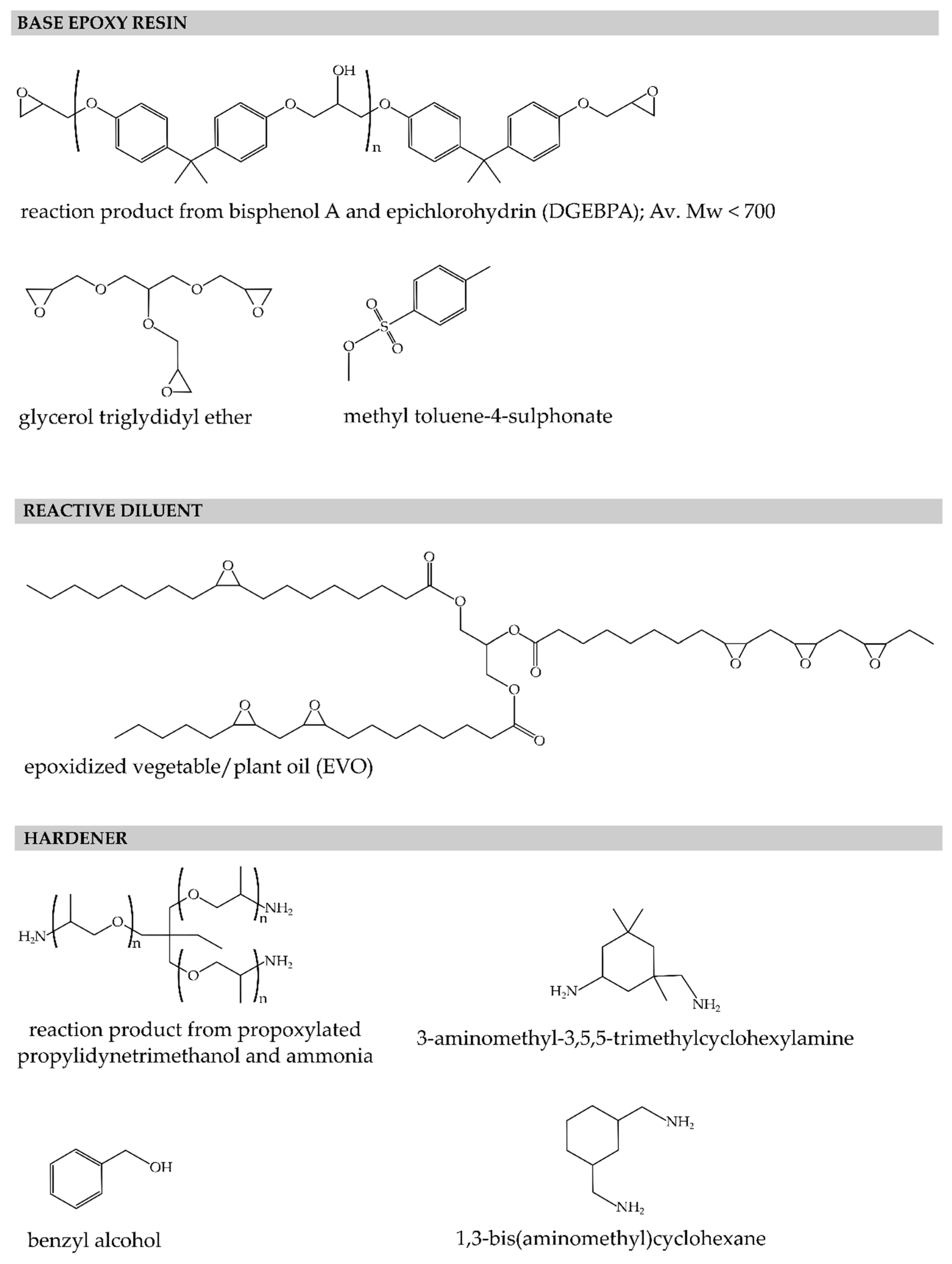
3.1. Materials
3.2. Differential Scanning Calorimetry (DSC) Kinetic Measurements
4. Results and Discussion
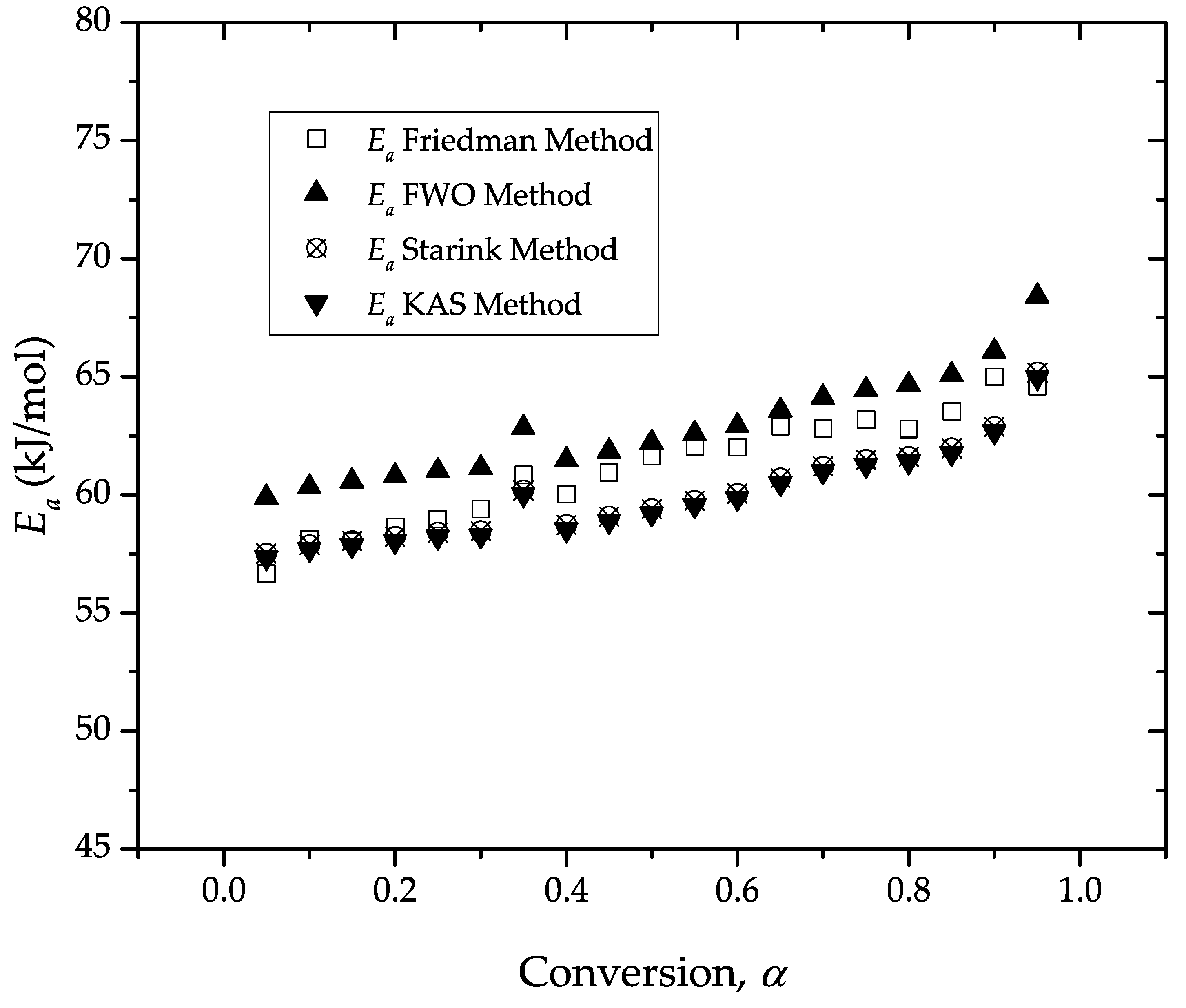
Estimation of the Apparent Activation Energy, Ea
5. Conclusions
Author Contributions
Funding
Conflicts of Interest
References
- Jin, F.L.; Li, X.; Park, S.J. Synthesis and application of epoxy resins: A review. J. Ind. Eng. Chem. 2015, 29, 1–11. [Google Scholar] [CrossRef]
- Ratna, D.; Patri, M.; Chakraborty, B.C.; Deb, P.C. Amine-Terminated Polysulfone as Modifier for Epoxy Resin. J. Appl. Polym. Sci. 1997, 65, 901–907. [Google Scholar] [CrossRef]
- David, R.; Raja, V.S.; Singh, S.K.; Gore, P. Development of anti-corrosive paint with improved toughness using carboxyl terminated modified epoxy resin. Prog. Org. Coat. 2018, 120, 58–70. [Google Scholar] [CrossRef]
- Minty, R.F.; Thomason, J.L.; Yang, L.; Stanley, W.; Roy, A. Development and application of novel technique for characterising the cure shrinkage of epoxy resins. Polym. Test. 2019, 73, 316–326. [Google Scholar] [CrossRef]
- François, C.; Pourchet, S.; Boni, G.; Rautiainen, S.; Samec, J.; Fournier, L.; Robert, C.; Thomas, C.M.; Fontaine, S.; Gaillard, Y.; et al. Design and synthesis of biobased epoxy thermosets from biorenewable resources. C. R. Chim. 2017, 20, 1006–1016. [Google Scholar] [CrossRef]
- Zabihi, O.; Ahmadi, M.; Nikafshar, S.; Chandrakumar Preyeswary, K.; Naebe, M. A technical review on epoxy-clay nanocomposites: Structure, properties, and their applications in fiber reinforced composites. Compos. Part B Eng. 2018, 135, 1–24. [Google Scholar] [CrossRef]
- Jin, H.; Miller, G.M.; Sottos, N.R.; White, S.R. Fracture and fatigue response of a self-healing epoxy adhesive. Polymer 2011, 52, 1628–1634. [Google Scholar] [CrossRef]
- Jin, H.; Miller, G.M.; Pety, S.J.; Griffin, A.S.; Stradley, D.S.; Roach, D.; Sottos, N.R.; White, S.R. Fracture behavior of a self-healing, toughened epoxy adhesive. Int. J. Adhes. Adhes. 2013, 44, 157. [Google Scholar] [CrossRef]
- Ramezanzadeh, B.; Niroumandrad, S.; Ahmadi, A.; Mahdavian, M.; Mohamadzadeh Moghadam, M.H. Enhancement of barrier and corrosion protection performance of an epoxy coating through wet transfer of amino functionalized graphene oxide. Corros. Sci. 2016, 103, 283–304. [Google Scholar] [CrossRef]
- Zhang, S.Y.; Ding, Y.F.; Li, S.J.; Luo, X.W.; Zhou, W.F. Effect of polymeric structure on the corrosion protection of epoxy coatings. Corros. Sci. 2002, 44, 861–869. [Google Scholar] [CrossRef]
- Yi, C.; Rostron, P.; Vahdati, N.; Gunister, E.; Alfantazi, A. Curing kinetics and mechanical properties of epoxy based coatings: The influence of added solvent. Prog. Org. Coat. 2018, 124, 165–174. [Google Scholar] [CrossRef]
- Zhao, X.; Li, Y.; Chen, W.; Li, S.; Zhao, Y.; Du, S. Improved fracture toughness of epoxy resin reinforced with polyamide 6/graphene oxide nanocomposites prepared via in situ polymerization. Compos. Sci. Technol. 2019, 171, 180–189. [Google Scholar] [CrossRef]
- Ho, T.H.; Wang, C.S. Modification of epoxy resins with polysiloxane thermoplastic polyurethane for electronic encapsulation: 1. Polymer 1996, 37, 2733–2742. [Google Scholar] [CrossRef]
- Loccufier, E.; Geltmeyer, J.; Daelemans, L.; D’Hooge, D.R.; De Buysser, K.; De Clerck, K. Silica Nanofibrous Membranes for the Separation of Heterogeneous Azeotropes. Adv. Funct. Mater. 2018, 28, 1804138. [Google Scholar] [CrossRef]
- Riemenschneider, W.; Bolt, H.M. Esters, Organic, Ullmann’s Encyclopedia of Industrial Chemistry; Wiley Online Library-VCH: Freeport, TX, USA, 2005; p. 8676. [Google Scholar]
- Dell’Erba, I.E.; Williams, R.J.J. Homopolymerization of epoxy monomers initiated by 4-(dimethylamino)pyridine. Polym. Eng. Sci. 2006, 46, 351–359. [Google Scholar] [CrossRef]
- Francis, B.; Lakshmana Rao, V.; Jose, S.; Catherine, B.K.; Ramaswamy, R.; Jose, J.; Thomas, S. Poly(ether ether ketone) with pendent methyl groups as a toughening agent for amine cured DGEBA epoxy resin. J. Mater. Sci. 2006, 41, 5467–5479. [Google Scholar] [CrossRef]
- Li, L.; Yu, Y.; Wu, Q.; Zhan, G.; Li, S. Effect of chemical structure on the water sorption of amine-cured epoxy resins. Corros. Sci. 2009, 51, 3000–3006. [Google Scholar] [CrossRef]
- Bell, J.P.; Carolina, N.P. Structure of a typical amine-cured epoxy resin. Polymer 1970, 6, 417. [Google Scholar] [CrossRef]
- Ellis, B.; Ashcroft, W.R.; Shaw, S.J.; Cantwell, W.J.; Kausch, H.H.; Johari, G.P.; Jones, F.R.; Chen, X.M. Chemistry and Technology of Epoxy Resins; Blackie Academic & Professional: London, UK, 1993. [Google Scholar]
- Bertomeu, D.; García-Sanoguera, D.; Fenollar, O.; Boronat, T.; Balart, R. Use of Eco-Friendly Epoxy Resins From Renewable Resources as Potential Substitutes of Petrochemical Epoxy Resins for Ambient Cured Composites with Flax Reinforcements. Polym. Compos. 2012, 33, 683–692. [Google Scholar] [CrossRef]
- Samper, M.D.; Petrucci, R.; Sánchez-Nacher, L.; Balart, R.; Kenny, J.M. New environmentally friendly composite laminates with epoxidized linseed oil (ELO) and slate fiber fabrics. Compos. Part B Eng. 2015, 71, 203–209. [Google Scholar] [CrossRef] [Green Version]
- Samper, M.D.; Petrucci, R.; Sanchez-Nacher, L.; Balart, R.; Kenny, J.M. Properties of composite laminates based on basalt fibers with epoxidized vegetable oils. Mater. Des. 2015, 72, 9–15. [Google Scholar] [CrossRef] [Green Version]
- España, J.M.; Sánchez-Nacher, L.; Boronat, T.; Fombuena, V.; Balart, R. Properties of biobased epoxy resins from epoxidized soybean oil (ESBO) cured with maleic anhydride (MA). JAOCS J. Am. Oil Chem. Soc. 2012, 89, 2067–2075. [Google Scholar] [CrossRef]
- Samper, M.D.; Petrucci, R.; Sánchez-Nacher, L.; Balart, R.; Kenny, J.M. Effect of silane coupling agents on basalt fiber-epoxidized vegetable oil matrix composite materials analyzed by the single fiber fragmentation technique. Polym. Compos. 2015, 36, 1205–1212. [Google Scholar] [CrossRef]
- Raquez, J.M.; Deléglise, M.; Lacrampe, M.F.; Krawczak, P. Thermosetting (bio)materials derived from renewable resources: A critical review. Prog. Polym. Sci. (Oxf.) 2010, 35, 487–509. [Google Scholar] [CrossRef]
- Meier, M.A.R.; Metzger, J.O.; Schubert, U.S. Plant oil renewable resources as green alternatives in polymer science. Chem. Soc. Rev. 2007, 36, 1788. [Google Scholar] [CrossRef] [PubMed]
- Stemmelen, M.; Pessel, F.; Lapinte, V.; Caillol, S.; Habas, J.P.; Robin, J.J. A fully biobased epoxy resin from vegetable oils: From the synthesis of the precursors by thiol-ene reaction to the study of the final material. J. Polym. Sci. Part A Polym. Chem. 2011, 49, 2434–2444. [Google Scholar] [CrossRef]
- Michałowicz, J. Bisphenol A—Sources, toxicity and biotransformation. Environ. Toxicol. Pharmacol. 2014, 37, 738–758. [Google Scholar] [CrossRef] [PubMed]
- Carbonell-Verdu, A.; Bernardi, L.; Garcia-Garcia, D.; Sanchez-Nacher, L.; Balart, R. Development of environmentally friendly composite matrices from epoxidized cottonseed oilv. Eur. Polym. J. 2015, 63, 1–10. [Google Scholar] [CrossRef]
- Ortiz, R.A.; López, D.P.; Cisneros, M.D.L.G.; Valverde, J.C.R.; Crivello, J.V. A kinetic study of the acceleration effect of substituted benzyl alcohols on the cationic photopolymerization rate of epoxidized natural oils. Polymer 2005, 46, 1535–1541. [Google Scholar] [CrossRef]
- Biermann, U.; Friedt, W.; Lang, S. New syntheses with oils and fats as renewable raw materials for the chemical industry. Angew. Chem. 2000, 39, 2206–2224. [Google Scholar] [CrossRef]
- Khot, S.N.; Lascala, J.J.; Can, E.; Morye, S.S.; Williams, G.I.; Palmese, G.R.; Kusefoglu, S.H.; Wool, R.P. Development and application of triglyceride-based polymers and composites. J. Appl. Polym. Sci. 2001, 82, 703–723. [Google Scholar] [CrossRef]
- Ferri, J.M.; Samper, M.D.; García-Sanoguera, D.; Reig, M.J.; Fenollar, O.; Balart, R. Plasticizing effect of biobased epoxidized fatty acid esters on mechanical and thermal properties of poly(lactic acid). J. Mater. Sci. 2016, 51, 5356–5366. [Google Scholar] [CrossRef] [Green Version]
- Carbonell-Verdu, A.; Garcia-Sanoguera, D.; Jordá-Vilaplana, A.; Sanchez-Nacher, L.; Balart, R. A new biobased plasticizer for poly(vinyl chloride) based on epoxidized cottonseed oil. J. Appl. Polym. Sci. 2016, 133, 1. [Google Scholar] [CrossRef]
- Fenollar, O.; Garcia-Sanoguera, D.; Sanchez-Nacher, L.; Lopez, J.; Balart, R. Effect of the epoxidized linseed oil concentration as natural plasticizer in vinyl plastisols. J. Mater. Sci. 2010, 45, 4406–4413. [Google Scholar] [CrossRef]
- Fenollar, O.; Garcia-Sanoguera, D.; Sánchez-Nácher, L.; López, J.; Balart, R. Characterization of the curing process of vinyl plastisols with epoxidized linseed oil as a natural-based plasticizer. J. Appl. Polym. Sci. 2012, 124, 2550–2557. [Google Scholar] [CrossRef]
- Samper, M.D.; Fombuena, V.; Boronat, T.; García-Sanoguera, D.; Balart, R. Thermal and mechanical characterization of epoxy resins (ELO and ESO) cured with anhydrides. JAOCS J. Am. Oil Chem. Soc. 2012, 89, 1521–1528. [Google Scholar] [CrossRef]
- Park, S.J.; Jin, F.L.; Lee, J.R. Effect of biodegradable epoxidized castor oil on physicochemical and mechanical properties of epoxy resins. Macromol. Chem. Phys. 2004, 205, 2048–2054. [Google Scholar] [CrossRef]
- Pawar, M.; Kadam, A.; Yemul, O.; Thamke, V.; Kodam, K. Biodegradable bioepoxy resins based on epoxidized natural oil (cottonseed & algae) cured with citric and tartaric acids through solution polymerization: A renewable approach. Ind. Crop. Prod. 2016, 89, 434–447. [Google Scholar]
- Incerti, D.; Wang, T.; Carolan, D.; Fergusson, A. Curing rate effects on the toughness of epoxy polymers. Polymer 2018, 159, 116–123. [Google Scholar] [CrossRef]
- Javdanitehran, M.; Berg, D.C.; Duemichen, E.; Ziegmann, G. An iterative approach for isothermal curing kinetics modelling of an epoxy resin system. Thermochim. Acta 2016, 623, 72–79. [Google Scholar] [CrossRef]
- Vyazovkin, S.; Burnham, A.K.; Criado, J.M.; Pérez-Maqueda, L.A.; Popescu, C.; Sbirrazzuoli, N. ICTAC Kinetics Committee recommendations for performing kinetic computations on thermal analysis data. Thermochim. Acta 2011, 520, 1–19. [Google Scholar] [CrossRef]
- Friedman, H.L. Kinetics of thermal degradation of char-forming plastics from thermogravimetry. Application to a phenolic plastic. J. Polym. Sci. Part C Polym. Symp. 2007, 6, 183–195. [Google Scholar] [CrossRef]
- Doyle, C.D. Estimating isothermal life from thermogravimetric data. J. Appl. Polym. Sci. 1962, 6, 639–642. [Google Scholar] [CrossRef]
- Akahira, T.; Sunose, T. Transactions of Joint Convention of Four Electrical Institutes; Chiba Institute of Technology: Chiba, Japan, 1969; p. 246. [Google Scholar]
- Starink, M.J. The determination of activation energy from linear heating rate experiments: A comparison of the accuracy of isoconversion methods. Thermochim. Acta 2003, 404, 163–176. [Google Scholar] [CrossRef]
- Kissinger, H.E. Variation of peak temperature with heating rate in differential thermal analysis. J. Res. Natl. Bur. Stand. 1956, 57, 217–221. [Google Scholar] [CrossRef]
- Farjas, J.; Butchosa, N.; Roura, P. A simple kinetic method for the determination of the reaction model from non-isothermal experiments. J. Therm. Anal. Calorim. 2010, 102, 615–625. [Google Scholar] [CrossRef]
- D’hooge, D.R.; Van Steenberge, P.H.M.; Reyniers, M.-F.; Marin, G.B. The strength of multi-scale modeling to unveil the complexity of radical polymerization. Prog. Polym. Sci. 2016, 58, 59–89. [Google Scholar] [CrossRef]
- Málek, J. The kinetic analysis of non-isothermal data. Thermochim. Acta 1992, 200, 257. [Google Scholar] [CrossRef]
- Senum, G.I.; Yang, R.T. Rational approximations of the integral of the Arrhenius function. J. Therm. Anal. 1977, 11, 445–447. [Google Scholar] [CrossRef]
- Pérez-Maqueda, L.A.; Criado, J.M. Accuracy of Senum and Yang’s approximations to the Arrhenius integral. J. Therm. Anal. Calorim. 2000, 60, 909–915. [Google Scholar] [CrossRef]
- Flynn, J.H. The “temperature integral”—Its use and abuse. Thermochim. Acta 1997, 300, 83–92. [Google Scholar] [CrossRef]
- Vyazovkin, S.; Chrissafis, K.; Di Lorenzo, M.L.; Koga, N.; Pijolat, M.; Roduit, B.; Sbirrazzuoli, N.; Suñol, J.J. ICTAC Kinetics Committee recommendations for collecting experimental thermal analysis data for kinetic computations. Thermochim. Acta 2014, 590, 1–23. [Google Scholar] [CrossRef]
- Hale, A.; Macosko, C.W.; Bair, H.E. Glass Transition Temperature as a Function of Conversion in Thermosetting Polymers. Macromolecules 1991, 24, 2610–2621. [Google Scholar] [CrossRef]
- Vyazovkin, S.; Sbirrazzuoli, N. Isoconversional kinetic analysis of thermally stimulated processes in polymers. Macromol. Rapid Commun. 2006, 27, 1515–1532. [Google Scholar] [CrossRef]
- Criado, J.M.; Malek, J.; Ortega, A. Applicability of the Master Plots in Kinetic Analysis. Thermochim. Acta 1989, 147, 377–385. [Google Scholar] [CrossRef]
- Bilyeu, B.; Brostow, W.; Menard, K.P.K.P. Epoxy thermosets and their applications. III. Kinetic equations and models. J. Mater. Educ. 2001, 23, 189–204. [Google Scholar]
- Benedetti, A.; Fernandes, P.; Granja, J.L.; Sena-Cruz, J.; Azenha, M. Influence of temperature on the curing of an epoxy adhesive and its influence on bond behaviour of NSM-CFRP systems. Compos. Part B Eng. 2016, 89, 219–229. [Google Scholar] [CrossRef] [Green Version]
- Málek, J. A computer program for kinetic analysis of non-isothermal thermoanalytical data. Thermochim. Acta 1989, 138, 337–346. [Google Scholar] [CrossRef]


| Reaction Model | f(α) | g(α) | |
|---|---|---|---|
| P2/3 | Power law | 2/3α−1/2 | α3/2 |
| P2 | Power law | 2α1/2 | α1/2 |
| A2 | Avrami–Erofeev | 2(1 − α)[−ln(1 − α)]1/2 | [−ln(1 − α)]1/2 |
| D1 | Diffusion in one dimension | 1/2α−1 | α2 |
| D2 | Valensi equation | −[ln(1 − α)]−1 | (1 − α) ln (1 − α) + α |
| F1 | Mample first order. | (1 − α) | −ln(1 − α) |
| F2 | Random nucleation with two nuclei of individual particle | (1 − α)2 | (1 − α)−1 |
| Fn | n-order reaction | (1 − α)n | [(1 − α)1 − n − 1]/(n − 1) |
| Property | Resoltech® 1070 | Resoltech® 1074 | Uncured Mixture (100:35) |
|---|---|---|---|
| Density at 23 °C (g cm−3) | 1.18 | 0.96 | 1.22 |
| Viscosity at 23 °C (mPa·s) | 1750 | 50 | 700 |
| Heating Rate (K min−1) | First Heating Cycle | Second Heating Cycle | ||
|---|---|---|---|---|
| Tp (K) | Tg (K) | |||
| 2.5 | 351.5 | 0.401 | 373.9 | 368.8 |
| 5 | 361.9 | 0.425 | 366.5 | 367.7 |
| 10 | 373.2 | 0.408 | 305.5 | 365.5 |
| 20 | 388.9 | 0.417 | 285.8 | 364.1 |
| Heating Rate (K min−1) | ||
|---|---|---|
| 2.5 | 0.099 | 0.420 |
| 5 | 0.076 | 0.438 |
| 10 | 0.085 | 0.442 |
| 20 | 0.098 | 0.443 |
| Heating Rate (K min−1) | ln (A) (A in min−1) | m | n |
|---|---|---|---|
| 2.5 | 18.464 | 0.156 | 1.792 |
| 5 | 18.546 | 0.143 | 1.866 |
| 10 | 18.460 | 0.148 | 1.677 |
| 20 | 18.415 | 0.155 | 1.712 |
© 2019 by the authors. Licensee MDPI, Basel, Switzerland. This article is an open access article distributed under the terms and conditions of the Creative Commons Attribution (CC BY) license (http://creativecommons.org/licenses/by/4.0/).
Share and Cite
Lascano, D.; Quiles-Carrillo, L.; Balart, R.; Boronat, T.; Montanes, N. Kinetic Analysis of the Curing of a Partially Biobased Epoxy Resin Using Dynamic Differential Scanning Calorimetry. Polymers 2019, 11, 391. https://doi.org/10.3390/polym11030391
Lascano D, Quiles-Carrillo L, Balart R, Boronat T, Montanes N. Kinetic Analysis of the Curing of a Partially Biobased Epoxy Resin Using Dynamic Differential Scanning Calorimetry. Polymers. 2019; 11(3):391. https://doi.org/10.3390/polym11030391
Chicago/Turabian StyleLascano, Diego, Luis Quiles-Carrillo, Rafael Balart, Teodomiro Boronat, and Nestor Montanes. 2019. "Kinetic Analysis of the Curing of a Partially Biobased Epoxy Resin Using Dynamic Differential Scanning Calorimetry" Polymers 11, no. 3: 391. https://doi.org/10.3390/polym11030391