Analysis of Longitudinal Waves in Rod-Type Piezoelectric Phononic Crystals

Abstract

Phononic crystals can be used to control elastic waves due to their frequency bands. This paper analyzes the passive and active control as well as the dispersion properties of longitudinal waves in rod-type piezoelectric phononic crystals over large frequency ranges. Based on the Love rod theory for modeling the longitudinal wave motions in the constituent rods and the method of reverberation-ray matrix (MRRM) for deriving the member transfer matrices of the constituent rods, a modified transfer matrix method (MTMM) is proposed for the analysis of dispersion curves by combining with the Floquet–Bloch principle and for the calculation of transmission spectra. Numerical examples are provided to validate the proposed MTMM for analyzing the band structures in both low and high frequency ranges. The passive control of longitudinal-wave band structures is studied by discussing the influences of the electrode’s thickness, the Poisson’s effect and the elastic rod inserts in the unit cell. The influences of electrical boundaries (including electric-open, applied electric capacity, electric-short and applied feedback control conditions) on the band structures are investigated to illustrate the active control scheme. From the calculated comprehensive frequency spectra over a large frequency range, the dispersion properties of the characteristic longitudinal waves in rod-type piezoelectric phononic crystals are summarized.

1. Introduction

Phononic crystal, which refers to natural or artificial materials characterized by periodic modulations of elastic properties, was put forward about two decades ago [1]. Since then, it has been widely investigated for applications based on controlling elastic waves [2], because it possesses frequency bands.

To control longitudinal waves, rod-type phononic crystals have been proposed. For example, Asiri et al. [3] and Asiri [4] devised periodic passive struts and mounts, which are essentially rod-type elastic phononic crystals, to isolate undesirable longitudinal vibrations in the helicopters and automobiles, respectively. The investigations of longitudinal waves in rod-type elastic phononic crystals up to 2014 were reviewed in Guo and Fang [5]. Unfortunately, these periodic elastic rods can only control the propagation of longitudinal waves in a passive mode. That is, their band structures are totally fixed as long as the geometrical, material and boundary configurations of the unit cells are determined. The frequency bands may not always fit to the external excitations. Therefore, rod-type phononic crystals containing smart material components have been presented in order to control the longitudinal waves in an active mode. Their frequency bands can be adjusted by tuning the temperature [6,7], magnetic [8] or electric [9,10,11,12,13,14,15,16,17,18,19,20,21,22,23,24,25,26] field to suit the external excitations. Among these smart periodic rods, the periodic piezoelectric rods [9,10,11,12,13,14,15,16,17,18,19,20,21,22,23,24,25,26] have particularly been paid more attention, because the piezoelectric materials are widely used and the electric field is comparatively easier to control. Thus far, two kinds of rod-type piezoelectric phononic crystals have been presented to actively control longitudinal-wave bands via electromechanical coupling. One kind is formed by periodically bonding shunted piezoelectric patches on the host rod, and the other is shaped through periodically arranging the piezoelectric constituent rods [9]. The attenuation of longitudinal vibrations/waves in rods with periodic shunted piezoelectric patches have been studied by Thorp et al. [10], Chen et al. [11] and Lossouarn et al. [12,13] using the transfer matrix method (TMM). Here, we focus on the longitudinal vibrations/waves in periodically arranged piezoelectric rods. After Baz [9] proposed the seminal concept about active control of periodic structures, Singh et al. [14] illustrated the effectiveness of the periodic rod with piezoelectric actuators by analyzing the frequency bands and responses with the TMM. Asiri et al. [15] and Asiri [16,17] predicted the attenuation of longitudinal waves in periodic binary piezoelectric-elastic composite rods using the combination of spectral element method and TMM, and validated their analysis by experiment. Using the same TMM, Li et al. [18] and Wang et al. [19] analyzed the localization of frequency bands in randomly disordered periodic binary piezoelectric-elastic rods without and with initial stress, respectively. Recently, Degraeve et al. [20] proposed to use periodic electrical boundary conditions realized by periodically embedded electrodes to tune Bragg bands in uniform homogeneous piezoelectric rods. This kind of electrical charge Bragg band gap in cases of electric-open, external capacitances and electric-short boundary conditions was studied by an analytical method (AM), finite element method (FEM) and experimental measurements. The model of Degraeve et al. [20] was extended by Kutsenko et al. [21] to consider the negative capacitance and by Ponge et al. [22] to devise a tunable Fabry–Perot resonator whose performance was validated by TMM and FEM analysis as well as experiment. Degraeve et al. [23] also extended their previous model by considering the different electrodes in the unit cell with different electrical boundaries and studied the electrical charge Bragg bands of the new phononic crystal with a semi-analytical method and experiment. The extensions to a model with elastic rod insert in the unit cell and with negative external capacitance were conducted in Reference [24] using the previous AM, FEM and experiment. Kutsenko et al. [25] further studied the band structures of more general rod-type piezoelectric phononic crystals where the unit cell consists of several piezoelectric or elastic-piezoelectric rods by TMM. The effective constitutive parameters were also derived. Vasilenko and Rogacheva [26] provided the similar effective modulus and the electroelastic state equations of periodic piezoelectric and adhesive rods by the homogenization method.

Although the above-mentioned studies make the longitudinal-wave band structures of periodically arranged piezoelectric or elastic-piezoelectric rods relatively clear, to the authors’ knowledge, pending problems still exist in four aspects: (1) Few studies have analyzed the longitudinal-wave bands in the high frequency range. The first reason is that the analytical method, like the conventional TMM, is proposed on the basis of classical rod theory valid only within pretty low frequency range. The second one is that the numerical method, like the versatile FEM, may be inefficient for the high frequency analysis since large amount of elements and very small time step are required in this case. (2) The mechanical vibration of the electrodes and the Poisson’s effect of the constituent rods are neglected without understanding their influences. The influence of the elastic rod inserts on the band structures is not clear enough. (3) Two electrical control manners in general have been proposed, i.e., setting the external voltage through the feedback control gain [14,15,16,17] and tuning the external electric capacity [18,19,20,21,22,23,24,25,26], since the electric-open and electric-short conditions correspond to zero and infinity electric capacities, respectively. The connection and difference of the influences of the applied feedback control and of the applied electric capacity on the frequency bands are not known. (4) The wave dispersion property has been solely represented by the frequency–wavenumber dispersion curve. However, other forms of dispersion curves such as the frequency–wavelength and frequency–phase velocity spectra are also vital to convey wave dispersion properties in different perspectives and engineering practices [5].

Aiming at solving the above four pending problems, this paper presents a modified transfer matrix method (MTMM) to analyze the longitudinal waves in rod-type piezoelectric phononic crystals, whose unit cell consists of any number of piezoelectric or elastic-piezoelectric rods with electrodes covered on the ends of piezoelectric rods. The proposed MTMM combines the Love rod theory [27,28], [29] (pp. 139–142), [30], the method of reverberation-ray matrix (MRRM) [5] and the transfer matrix method (TMM) [14,15,16,17,18,19,21,22,25] to analyze the dispersion curves by considering the Floquet–Bloch theorem [31,32] and to calculate the transmission spectra. The Love rod theory is adopted to model the longitudinal wave motions in the piezoelectric, elastic and electrode constituent rods of the unit cell. The MRRM is utilized to derive the member transfer matrices of the constituent rods. Therefore, the proposed MTMM is effective over a large frequency range as long as the Love rod theory is valid, as illustrated by the numerical examples. The influences of the electrode’s thickness, the rods’ cross-sectional dimension, the elastic rod inserts and the applied electric capacity and the applied feedback control on the band structures are studied numerically. All the frequency-related dispersion curves are calculated to show comprehensively the dispersion properties of characteristic longitudinal waves in rod-type piezoelectric phononic crystals. This paper is organized as follows. Section 2 derives the formulation of the proposed MTMM. Numerical examples are given in Section 3 to validate the MTMM, to demonstrate the influences of the electrode’s thickness, the rods’ cross-sectional dimension and the elastic rod inserts for the passive control, to illustrate the influences of the applied electric capacity and feedback control for the active control, and to indicate all the frequency-related dispersion curves in both low and high frequency ranges. Section 4 draws conclusions.

2. Analysis of Longitudinal Waves in Rod-Type Piezoelectric Phononic Crystals with the MTMM

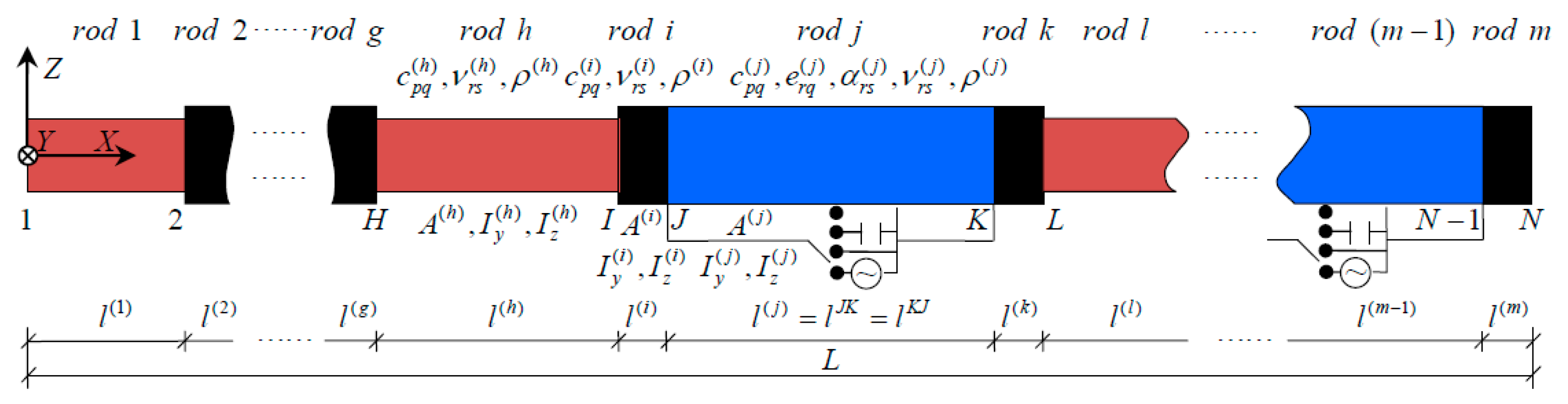
2.1. Basic Model

Consider a periodic piezoelectric composite rod with its unit cell consisting of alternate homogeneous piezoelectric and elastic rods as well as electrodes between them. The schematic of the unit cell is shown in Figure 1, where $m$ members and $N$ joints ($N=m+1$) are denoted from left to right by $1,2,\cdots ,i,j,\cdots ,(m-1),m$ and $1,2,\cdots ,I,J,K,\cdots ,(N-1),N$, respectively. All of the components are assumed to be rigidly connected. The piezoelectric rods are polarized along the length direction. The electrodes are covered at the ends of the piezoelectric rods, to which any of the four electrical boundaries (electric-open, applied electric capacity, electric-short and applied feedback control conditions) is imposed. Therefore, the longitudinal effect of the piezoelectric rods is utilized. Figure 1 also shows the pertinent physical and geometrical parameters of some typical constituent rods, where the Voigt notation (compressed matrix notation) is used for reducing the orders [33]. $c_{pq}^{(j)}$, $e_{rq}^{(j)}$, ${\alpha }_{rs}^{(j)}$, ${\nu }_{rs}^{(j)}$ ($p,q=1,2,3,4,5,6$, $r,s=1,2,3$) and ${\rho }^{(j)}$ are the elastic constants, the piezoelectric constants, the dielectric constants, the Poisson’s ratios and the material density of the piezoelectric rod $j$, respectively; $A^{(j)}$, $I_y^{(j)}$, $I_z^{(j)}$ and $l^{(j)}$ are the cross-sectional area, second moment of inertia about $y$ and $z$ axis and the rod length, respectively; $c_{pq}^{(h)}$, ${\nu }_{rs}^{(h)}$, ${\rho }^{(h)}$, $A^{(h)}$, $I_y^{(h)}$, $I_z^{(h)}$ and $l^{(h)}$ are the corresponding parameters of the elastic rod $h$; and $c_{pq}^{(i)}$, ${\nu }_{rs}^{(i)}$, ${\rho }^{(i)}$, $A^{(i)}$, $I_y^{(i)}$, $I_z^{(i)}$ and $l^{(i)}$ are those of the electrode $i$.

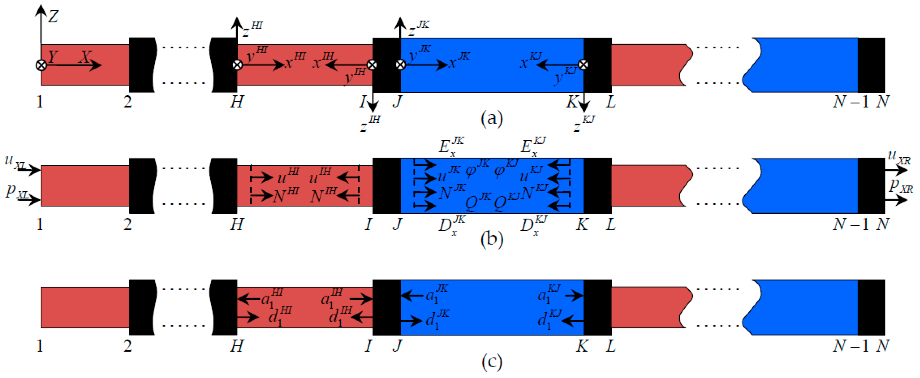
2.2. Coordinate Systems and Physical Variables

For the convenience of system and joint description, a global coordinates $(X,Y,Z)$ is set up as shown in Figure 2a. To facilitate the member description, a pair of dual local coordinates $(x^{JK},y^{JK},z^{JK})$ and $(x^{KJ},y^{KJ},z^{KJ})$ is set up for any typical member $j$ (also called $JK$ or $KJ$ in the pertaining coordinates), as also indicated in Figure 2a.

To make the later derivation clear, hereafter we use $u$, $v$ and $w$ to express the displacements of a particle along $x$, $y$ and $z$ axes, respectively. $f_x$, $f_y$ and $f_z$ are used to represent the specified forces along $x$, $y$ and $z$ axes of a surface particle, respectively. The resulting axial force at a cross-section of the constituent rod is denoted by $N$. $u_X$ and $p_X$ are the displacement and resulting external force at the unit cell ends along $X$ axis, respectively. For the electrical variables: $\phi$ is the electric potential at a cross-section of the constituent rod; $q$ is the electric charge density per surface area; and the total electric charge on a cross-section is denoted by $Q$.

In general, the axial displacements and forces are the fundamental physical variables to analyze the system, which are shown in Figure 2b. $u_{XL}$ ($u_{XR}$) and $p_{XL}$ ($p_{XR}$) denote the axial displacement and force of joint $1$ ($N$), respectively, which are described in coordinates $(X,Y,Z)$. The axial displacement and force of a typical member $j$ at cross-section $x^{JK}$ in $(x^{JK},y^{JK},z^{JK})$ are denoted by $u^{JK}(x^{JK})$ and $N^{JK}(x^{JK})$, respectively. Those physical variables can also be described in $(x^{KJ},y^{KJ},z^{KJ})$ as $u^{KJ}(x^{KJ})$ and $N^{KJ}(x^{KJ})$, respectively. For a piezoelectric constituent rod, say rod $j$, the electric field intensity and displacement as vector quantities as well as the electric potential and charge as scalar quantities are needed to be considered in the analysis. They are represented as $E_x^{JK}(x^{JK})$, $D_x^{JK}(x^{JK})$, ${\phi }^{JK}(x^{JK})$ and $Q^{JK}(x^{JK})$ in $(x^{JK},y^{JK},z^{JK})$ as well as $E_x^{KJ}(x^{KJ})$, $D_x^{KJ}(x^{KJ})$, ${\phi }^{KJ}(x^{KJ})$ and $Q^{KJ}(x^{KJ})$ in $(x^{KJ},y^{KJ},z^{KJ})$, respectively, as also given in Figure 2b. It should be noted that all the physical variables are deemed as positive when they are along the positive direction of the pertaining coordinate. During the following analysis, the generalized displacements and forces are expressed by the wave amplitudes, which are depicted in Figure 2c.

2.3. Governing Equations and Wave Solutions of a Constituent Rod

Based on the basic idea of Love rod theory [27,28], [29] (pp. 139–142), [30], which considers the Poisson’s effect, the time-domain equations governing the longitudinal wave motions in any of the constituent rods described in its dual local coordinates can be derived by Hamilton principle [29] (pp. 126–131), [34]. The assumptions of the Love rod with considering the Poisson’s effect include: (1) The axial displacement (electric potential) is uniformly distributed on any cross-section of the rod. Hence, the axial displacement (electric potential) at the centroid is used to represent that of the whole cross-section. (2) The two lateral displacements are linearly distributed on the cross-section. They are zero at the centroid and alter linearly with the corresponding coordinates. The proportional coefficients are the multiplication of the corresponding Poisson’s ratios with the axial strain of that cross-section. Apply these assumptions and the three-dimensional elasticity [33,34], [35] (pp. 57–60), the derivation for a piezoelectric rod is detailed in Appendix A, and that for an elastic rod which representing any of the elastic rods and the electrodes is briefed in Appendix B.

For any piezoelectric rod in the unit cell, say member $j$, applying Fourier transform [36] (p. 725) to the time-domain governing equations and constitutive relations, as given in Equations (A12) and (A11), leads to the frequency-domain counterparts as

$$\left[(c+e^2/\alpha )A-\rho ({\nu }_{12}^2{I}_z+{\nu }_{13}^2{I}_y){\omega }^2\right]\frac{{\mathrm{d}}^2\widehat{u}}{\mathrm{d}{x}^2}+\rho A{\omega }^2\widehat{u}=0$$

(1)

$$\widehat{N}=\left[cA-\rho ({\nu }_{12}^2{I}_z+{\nu }_{13}^2{I}_y){\omega }^2\right]\frac{\mathrm{d}\widehat{u}}{\mathrm{d}x}+eA\frac{\mathrm{d}\widehat{\phi }}{\mathrm{d}x}, \widehat{Q}=-eA\frac{\mathrm{d}\widehat{u}}{\mathrm{d}x}+\alpha A\frac{\mathrm{d}\widehat{\phi }}{\mathrm{d}x}$$

(2)

where $\omega$ is the circular frequency and a caret over a physical variable signifies the corresponding quantity in the frequency domain here and after. $\widehat{u}$ ($\widehat{N}$) and $\widehat{\phi }$ ($\widehat{Q}$) are the axial displacement (force) and the electric potential (charge) at any cross-section $x$, respectively. $c$, $e$ and $\alpha$, as given in Appendix A, are the equivalent elastic, piezoelectric and dielectric constants, respectively; $\rho$ is the material density; ${\nu }_{12}$ (${\nu }_{13}$) and $I_y$ ($I_z$) are the Poisson’s ratio and the cross-sectional moment of inertia with respect to $y$ ($z$) axis, respectively; and $A$ is the cross-sectional area. When $\widehat{Q}=-{\widehat{D}}_{x}A$ is deemed as the scalar electric charge at the initial end of the piezoelectric rod with ${\widehat{D}}_x$ the uniform electric displacement, the second formula of Equation (2) leads to

$$\frac{\mathrm{d}\widehat{\phi }}{\mathrm{d}x}=\frac{e}{\alpha }\frac{\mathrm{d}\widehat{u}}{\mathrm{d}x}+\frac{\widehat{Q}}{\alpha A}, \widehat{V}=\widehat{\phi }(l)-\widehat{\phi }(0)={\displaystyle {\int }_0^l\frac{\mathrm{d}\widehat{\phi }}{\mathrm{d}x}\mathrm{d}x}=\frac{e}{\alpha }\left[\widehat{u}(l)-\widehat{u}(0)\right]-{\displaystyle {\int }_0^l\frac{{\widehat{D}}_x}{\alpha }\mathrm{d}x}=\frac{e}{\alpha }\left[\widehat{u}(l)-\widehat{u}(0)\right]+\frac{\widehat{Q}l}{\alpha A}$$

(3)

where $\widehat{V}$ is the electric potential difference (electric voltage) between the two ends of the piezoelectric rod. Consider the associated mathematical formulas to the four electric boundary conditions, as shown in

Table 1. The expressions of involved electrical variables as formulas of mechanical variables.

Electrical Boundary Conditions	Associated Mathematical Formulas	Expressions of $\widehat{V}$	Expressions of $\widehat{Q}$
Electric-open	$\widehat{Q}=0$	$\frac{e}{\alpha }\left[\widehat{u}(l)-\widehat{u}(0)\right]$	$0$
Applied electric capacity	$\widehat{Q}=-C\widehat{V}$	$\frac{eA}{\alpha A+Cl}\left[\widehat{u}(l)-\widehat{u}(0)\right]$	$-\frac{eCA}{\alpha A+Cl}\left[\widehat{u}(l)-\widehat{u}(0)\right]$
Electric-short	$\widehat{V}=0$	$0$	$-\frac{eA}{l}\left[\widehat{u}(l)-\widehat{u}(0)\right]$
Applied feedback control	$\widehat{V}=-K_g\left[\widehat{u}(l)-\widehat{u}(0)\right]$	$-K_g\left[\widehat{u}(l)-\widehat{u}(0)\right]$	$-\frac{\alpha A}{l}\left(\frac{e}{\alpha }+K_g\right)\left[\widehat{u}(l)-\widehat{u}(0)\right]$
Electrical Boundary Conditions	Expressions of $\mathrm{d}\widehat{\phi }/\mathrm{d}x$		Expressions of $B$
Electric-open	$\frac{e}{\alpha }\frac{\mathrm{d}\widehat{u}}{\mathrm{d}x}$		$0$
Applied electric capacity	$\frac{e}{\alpha }\frac{\mathrm{d}\widehat{u}}{\mathrm{d}x}-\frac{e}{\alpha }\frac{C}{\alpha A+Cl}\left[\widehat{u}(l)-\widehat{u}(0)\right]$		$-\frac{e^{2}CA}{{\alpha }^{2}A+\alpha Cl}$
Electric-short	$\frac{e}{\alpha }\frac{\mathrm{d}\widehat{u}}{\mathrm{d}x}-\frac{e}{\alpha l}\left[\widehat{u}(l)-\widehat{u}(0)\right]$		$-\frac{e^{2}A}{\alpha l}$
Applied feedback control	$\frac{e}{\alpha }\frac{\mathrm{d}\widehat{u}}{\mathrm{d}x}-\frac{1}{l}\left(\frac{e}{\alpha }+K_g\right)\left[\widehat{u}(l)-\widehat{u}(0)\right]$		$-\frac{eA}{l}\left(\frac{e}{\alpha }+K_g\right)$

, the expressions of $\widehat{V}$, $\widehat{Q}$ and $\mathrm{d}\widehat{\phi }/\mathrm{d}x$ as formulas of mechanical variables can be obtained from Equation (3), which are also provided in Table 1. The specified electrical coefficients are external capacitance $C$ and control gain $K_g$ for the applied electric capacity and the applied feedback control conditions, respectively, while the electric-open and the electric-short conditions do not have specified electrical coefficient.

According to the theory of ordinary differential equations [36] (p. 503), the solution to the spectral axial displacement can be obtained directly from Equation (1). Substituting the above expressions of $\mathrm{d}\widehat{\phi }/\mathrm{d}x$ into the first formula of Equation (2) and then introducing the solution to the spectral axial displacement, one obtains the wave solution to the spectral axial force. These solutions are expressed as

$$\widehat{u}(x)=a_1{\mathrm{e}}^{\mathrm{i}{k}_{1}x}+d_1{\mathrm{e}}^{-\mathrm{i}{k}_{1}x}, \widehat{N}(x)={\zeta }_1{a}_1{\mathrm{e}}^{\mathrm{i}{k}_{1}x}-{\zeta }_1{d}_1{\mathrm{e}}^{-\mathrm{i}{k}_{1}x}+B\left[\widehat{u}(l)-\widehat{u}(0)\right]$$

(4)

where $\mathrm{i}=\sqrt{-1}$ is the imaginary unit. The first and the second terms in the two formulas of Equation (4), when combining with the kernel function ${\mathrm{e}}^{\mathrm{i}\omega t}$ of the Fourier transform [36] (p. 725), represent waves traveling along the negative and positive $x$-axis that are called as the arriving and departing waves, respectively. $a_1$ and $d_1$ are the corresponding undetermined wave amplitudes. $k_1=\omega /c_1$ and $c_1=\sqrt{[(c+e^2/\alpha )A-\rho ({\nu }_{12}^2{I}_z+{\nu }_{13}^2{I}_y){\omega }^2]/\rho A}$ are the wave number and wave speed, respectively. ${\zeta }_1=\mathrm{i}{k}_1[(c+e^2/\alpha )A-\rho ({\nu }_{12}^2{I}_z+{\nu }_{13}^2{I}_y){\omega }^2]=\mathrm{i}\omega \sqrt{\rho A[(c+e^2/\alpha )A-\rho ({\nu }_{12}^2{I}_z+{\nu }_{13}^2{I}_y){\omega }^2]}$ and $B$ are the axial-force influence coefficients of the piezoelectric rod that are irrelative and relative to the electrical boundary condition, respectively. The expressions of $B$ for the four electrical boundary conditions are also shown in Table 1. It should be noted in Table 1 that as ($C=\infty$ or $K_g=0$), all the solutions to $\widehat{V}$, $\widehat{Q}$, $\mathrm{d}\widehat{\phi }/\mathrm{d}x$ and $B$ for the applied electric capacity (applied electric capacity or applied feedback control) condition are degenerated to the corresponding ones for the electric open (short) circuit condition.

For any elastic rod (or electrode) in the unit cell, say member $h$ (or $i$), the frequency-domain governing equation and constitutive relation are obtained by Fourier transform [36] (p. 725) to their time-domain counterparts, as given in Equations (A17) and (A18)

$$\left[cA-\rho ({\nu }_{12}^2{I}_z+{\nu }_{13}^2{I}_y){\omega }^2\right]\frac{{\mathrm{d}}^2\widehat{u}}{\mathrm{d}{x}^2}+\rho A{\omega }^2\widehat{u}=0$$

(5)

$$\widehat{N}=\left[cA-\rho ({\nu }_{12}^2{I}_z+{\nu }_{13}^2{I}_y){\omega }^2\right]\frac{\mathrm{d}\widehat{u}}{\mathrm{d}x}$$

(6)

respectively. From these equations, the wave solutions to the axial displacement and force of an elastic rod (or electrode) are directly obtained as

$$\widehat{u}(x)=a_1{\mathrm{e}}^{\mathrm{i}{k}_{1}x}+d_1{\mathrm{e}}^{-\mathrm{i}{k}_{1}x}, \widehat{N}(x)={\zeta }_1{a}_1{\mathrm{e}}^{\mathrm{i}{k}_{1}x}-{\zeta }_1{d}_1{\mathrm{e}}^{-\mathrm{i}{k}_{1}x}$$

(7)

where $k_1=\omega /\sqrt{[cA-\rho ({\nu }_{12}^2{I}_z+{\nu }_{13}^2{I}_y){\omega }^2]/\rho A}$ and ${\zeta }_1=\mathrm{i}{k}_1[cA-\rho ({\nu }_{12}^2{I}_z+{\nu }_{13}^2{I}_y){\omega }^2]$ should be noted, and all the other quantities are identical to those for the piezoelectric rod.

2.4. Transfer Matrix of a Member

Based on the concept of MRRM [5], the transfer matrix of a structural member, which relates the axial displacement and force of one end with those of the other, can be derived.

For any piezoelectric rod in the unit cell, say member $j$, the wave solutions to the axial displacements and forces in the dual coordinates $(x^{JK},y^{JK},z^{JK})$ and $(x^{KJ},y^{KJ},z^{KJ})$ can be written from Equation (4). When the constants satisfying ${\Gamma }^{JK}={\Gamma }^{KJ}={\Gamma }^{(j)}$ ($\Gamma =k_1,{\zeta }_1,B,l$) is noticed, these wave solutions are expressed as

$$\begin{gathered} \left\{\begin{array}{c}{\widehat{u}}^{JK}(x^{JK})\\ {\widehat{N}}^{JK}(x^{JK})\end{array}\right\}=\left[\begin{array}{cc}1& 1\\ {\zeta }_1^{(j)}& -{\zeta }_1^{(j)}\end{array}\right]\left[\begin{array}{cc}{\mathrm{e}}^{\mathrm{i}{k}_1^{(j)}{x}^{JK}}& 0\\ 0& {\mathrm{e}}^{-\mathrm{i}{k}_1^{(j)}{x}^{JK}}\end{array}\right]\left\{\begin{array}{c}{a}_1^{JK}\\ d_1^{JK}\end{array}\right\}+\left[\begin{array}{cc}0& 0\\ -B^{(j)}& B^{(j)}\end{array}\right]\left\{\begin{array}{c}{\widehat{u}}^{JK}(0)\\ {\widehat{u}}^{JK}(l^{(j)})\end{array}\right\} \\ \left\{\begin{array}{c}{\widehat{u}}^{KJ}(x^{KJ})\\ {\widehat{N}}^{KJ}(x^{KJ})\end{array}\right\}=\left[\begin{array}{cc}1& 1\\ {\zeta }_1^{(j)}& -{\zeta }_1^{(j)}\end{array}\right]\left[\begin{array}{cc}{\mathrm{e}}^{\mathrm{i}{k}_1^{(j)}{x}^{KJ}}& 0\\ 0& {\mathrm{e}}^{-\mathrm{i}{k}_1^{(j)}{x}^{KJ}}\end{array}\right]\left\{\begin{array}{c}{a}_1^{KJ}\\ d_1^{KJ}\end{array}\right\}+\left[\begin{array}{cc}0& 0\\ -B^{(j)}& B^{(j)}\end{array}\right]\left\{\begin{array}{c}{\widehat{u}}^{KJ}(0)\\ {\widehat{u}}^{KJ}(l^{(j)})\end{array}\right\} \end{gathered}$$

(8)

Due to the uniqueness of the physical variables at any cross section ($x^{JK}=l^{(j)}-x^{KJ}$) of a typical member $JK$, compatibility conditions exist between the displacement (force) expressed in the dual local coordinates

$${\widehat{u}}^{JK}(x^{JK})=-{\widehat{u}}^{KJ}(l^{(j)}-x^{JK}), {\widehat{N}}^{JK}(x^{JK})={\widehat{N}}^{KJ}(l^{(j)}-x^{JK})$$

(9)

Substituting Equation (8) into Equation (9) gives the phase relations of the typical member $j$

$$a_1^{JK}=-{\mathrm{e}}^{-\mathrm{i}{k}_1^{(j)}{l}^{(j)}}{d}_1^{KJ}, a_1^{KJ}=-{\mathrm{e}}^{-\mathrm{i}{k}_1^{(j)}{l}^{(j)}}{d}_1^{JK}$$

(10)

By noticing ${\widehat{u}}^{JK}(l^{(j)})=-{\widehat{u}}^{KJ}(0)$ and ${\widehat{u}}^{KJ}(l^{(j)})=-{\widehat{u}}^{JK}(0)$, letting $x^{JK}=0$ and $x^{KJ}=0$ in Equation (8), and then introducing Equation (10) into the resulting equation, one obtains the relations between the displacements/forces at the member ends and the departing wave amplitudes

$$\begin{gathered} \left\{\begin{array}{c}{\widehat{u}}^{JK}(0)\\ {\widehat{N}}^{JK}(0)\end{array}\right\}=\left[\begin{array}{cc}1& -{\mathrm{e}}^{-\mathrm{i}{k}_1^{(j)}{l}^{(j)}}\\ [B^{(j)}{\mathrm{e}}^{-\mathrm{i}{k}_1^{(j)}{l}^{(j)}}-({\zeta }_1^{(j)}+B^{(j)})]& [-({\zeta }_1^{(j)}-B^{(j)}){\mathrm{e}}^{-\mathrm{i}{k}_1^{(j)}{l}^{(j)}}-B^{(j)}]\end{array}\right]\left\{\begin{array}{c}{d}_1^{JK}\\ d_1^{KJ}\end{array}\right\} \\ \left\{\begin{array}{c}{\widehat{u}}^{KJ}(0)\\ {\widehat{N}}^{KJ}(0)\end{array}\right\}=\left[\begin{array}{cc}-{\mathrm{e}}^{-\mathrm{i}{k}_1^{(j)}{l}^{(j)}}& 1\\ [-({\zeta }_1^{(j)}-B^{(j)}){\mathrm{e}}^{-\mathrm{i}{k}_1^{(j)}{l}^{(j)}}-B^{(j)}]& [B^{(j)}{\mathrm{e}}^{-\mathrm{i}{k}_1^{(j)}{l}^{(j)}}-({\zeta }_1^{(j)}+B^{(j)})]\end{array}\right]\left\{\begin{array}{c}{d}_1^{JK}\\ d_1^{KJ}\end{array}\right\} \end{gathered}$$

(11)

Eliminating the departing wave amplitudes from Equation (11), one obtains the transfer relation of the typical piezoelectric member $j$

$$\left\{\begin{array}{c}{\widehat{u}}^{KJ}(0)\\ {\widehat{N}}^{KJ}(0)\end{array}\right\}=T^{(j)}\left\{\begin{array}{c}{\widehat{u}}^{JK}(0)\\ {\widehat{N}}^{JK}(0)\end{array}\right\}=\frac{1}{\Delta }\left[\begin{array}{cc}{t}_{11}& t_{12}\\ t_{21}& t_{22}\end{array}\right]\left\{\begin{array}{c}{\widehat{u}}^{JK}(0)\\ {\widehat{N}}^{JK}(0)\end{array}\right\}$$

(12)

where $T^{(j)}$ is the transfer matrix of piezoelectric member $j$. The quantities forming $T^{(j)}$ are

$$\begin{gathered} \Delta =-B^{(j)}({\mathrm{e}}^{-2\mathrm{i}{k}_1^{(j)}{l}^{(j)}}-1)+2{\zeta }_1^{(j)}{\mathrm{e}}^{-\mathrm{i}{k}_1^{(j)}{l}^{(j)}}, t_{11}=-t_{22}=-({\zeta }_1^{(j)}-B^{(j)}){\mathrm{e}}^{-2\mathrm{i}{k}_1^{(j)}{l}^{(j)}}-({\zeta }_1^{(j)}+B^{(j)}) \\ {t}_{12}={\mathrm{e}}^{-2\mathrm{i}{k}_1^{(j)}{l}^{(j)}}-1, t_{21}=-{({\zeta }_1^{(j)})}^2({\mathrm{e}}^{-2\mathrm{i}{k}_1^{(j)}{l}^{(j)}}-1)+2{\zeta }_1^{(j)}{B}^{(j)}{({\mathrm{e}}^{-\mathrm{i}{k}_1^{(j)}{l}^{(j)}}-1)}^2 \end{gathered}$$

(13)

The transfer relation of any elastic rod (electrode) in the unit cell, say member $h$ ($i$), can be derived by starting from Equation (7) and then using a similar way as that for the piezoelectric member $j$. It can be expressed as the same form as Equation (12), but the quantities building the member transfer matrix $T^{(\Pi )}$ ($\Pi =h,i$) should be

$$\Delta =2{\zeta }_1^{(\Pi )}{\mathrm{e}}^{-\mathrm{i}{k}_1^{(\Pi )}{l}^{(\Pi )}}, t_{11}=-t_{22}=-{\zeta }_1^{(\Pi )}({\mathrm{e}}^{-2\mathrm{i}{k}_1^{(\Pi )}{l}^{(\Pi )}}+1), t_{12}={\mathrm{e}}^{-2\mathrm{i}{k}_1^{(\Pi )}{l}^{(\Pi )}}-1, t_{21}=-{({\zeta }_1^{(\Pi )})}^2({\mathrm{e}}^{-2\mathrm{i}{k}_1^{(\Pi )}{l}^{(\Pi )}}-1)$$

(14)

Please note that if the single local coordinates (other than the dual local coordinates) is used to describe a structural member, the conventional member transfer matrix can be derived. Its components are

$$\begin{gathered} \Delta =-B^{(j)}({\mathrm{e}}^{-\mathrm{i}{k}_1^{(j)}{l}^{(j)}}-{\mathrm{e}}^{\mathrm{i}{k}_1^{(j)}{l}^{(j)}})+2{\zeta }_1^{(j)}, t_{11}=t_{22}=({\zeta }_1^{(j)}-B^{(j)}){\mathrm{e}}^{-\mathrm{i}{k}_1^{(j)}{l}^{(j)}}+({\zeta }_1^{(j)}+B^{(j)}){\mathrm{e}}^{\mathrm{i}{k}_1^{(j)}{l}^{(j)}} \\ {t}_{12}=-({\mathrm{e}}^{-\mathrm{i}{k}_1^{(j)}{l}^{(j)}}-{\mathrm{e}}^{\mathrm{i}{k}_1^{(j)}{l}^{(j)}}), t_{21}=-{({\zeta }_1^{(j)})}^2({\mathrm{e}}^{-\mathrm{i}{k}_1^{(j)}{l}^{(j)}}-{\mathrm{e}}^{\mathrm{i}{k}_1^{(j)}{l}^{(j)}})+2{\zeta }_1^{(j)}{B}^{(j)}({\mathrm{e}}^{-\mathrm{i}{k}_1^{(j)}{l}^{(j)}}+{\mathrm{e}}^{\mathrm{i}{k}_1^{(j)}{l}^{(j)}}-2) \end{gathered}$$

(15)

for the typical piezoelectric rod $j$ and

$$\begin{gathered} \Delta =2{\zeta }_1^{(\Pi )}, t_{11}=t_{22}={\zeta }_1^{(\Pi )}({\mathrm{e}}^{-\mathrm{i}{k}_1^{(\Pi )}{l}^{(\Pi )}}+{\mathrm{e}}^{\mathrm{i}{k}_1^{(\Pi )}{l}^{(\Pi )}}), t_{12}=-({\mathrm{e}}^{-\mathrm{i}{k}_1^{(\Pi )}{l}^{(\Pi )}}-{\mathrm{e}}^{\mathrm{i}{k}_1^{(\Pi )}{l}^{(\Pi )}}) \\ {t}_{21}=-{({\zeta }_1^{(\Pi )})}^2({\mathrm{e}}^{-\mathrm{i}{k}_1^{(\Pi )}{l}^{(\Pi )}}-{\mathrm{e}}^{\mathrm{i}{k}_1^{(\Pi )}{l}^{(\Pi )}}) \end{gathered}$$

(16)

for the typical elastic rod $h$ or electrode $i$ ($\Pi =h,i$). Although the derivation of member transfer relations on the basis of members’ dual local coordinates in our MTMM seems tangled when compared with the process based on single local coordinates, it is noticed from the comparison of Equations (13) and (14) with Equations (15) and (16), respectively, that the so-derived member transfer matrices abstain from exponentially function in form of ${\mathrm{e}}^{+\mathrm{i}{k}_{1}l}$. Namely, in Equations (13) and (14), only exponential function in form of ${\mathrm{e}}^{-\mathrm{i}{k}_{1}l}$ is involved. However, in Equations (15) and (16), the exponential functions in form of ${\mathrm{e}}^{-\mathrm{i}{k}_{1}l}$ and ${\mathrm{e}}^{+\mathrm{i}{k}_{1}l}$ appear simultaneously.

2.5. Transfer Matrix of a Joint

At the external joint $1$, where the current unit cell is connected to the left adjacent unit cell, the compatibility condition between the member displacement and the joint displacement and the equilibrium condition between the member force and the joint force are combined to give the joint transfer relations

$$\left\{\begin{array}{c}{\widehat{u}}^{12}(0)\\ {\widehat{N}}^{12}(0)\end{array}\right\}=\left[\begin{array}{cc}1& 0\\ 0& 1\end{array}\right]\left\{\begin{array}{c}{\widehat{u}}_{XL}\\ -{\widehat{p}}_{XL}\end{array}\right\}=T^1\left\{\begin{array}{c}{\widehat{u}}_{XL}\\ -{\widehat{p}}_{XL}\end{array}\right\}=\left[\begin{array}{cc}1& 0\\ 0& -1\end{array}\right]\left\{\begin{array}{c}{\widehat{u}}_{XL}\\ {\widehat{p}}_{XL}\end{array}\right\}={\tilde{T}}^1\left\{\begin{array}{c}{\widehat{u}}_{XL}\\ {\widehat{p}}_{XL}\end{array}\right\}$$

(17)

where $T^1=I_2=<1,1>$ is the transfer matrix of external joint $1$ with $I_2$ denoting the identity matrix of second order, and $<\cdot >$ here and after denotes diagonal (or block diagonal) matrix. ${\tilde{T}}^1=<1,-1>$ is a variant of $T^1$ as ${\widehat{p}}_{XL}$ other than $-{\widehat{p}}_{XL}$ is used in the transfer relation.

At any internal joint that connects the neighboring constituent rods, the typical joint $K$ ($2\le K\le N-1$) for instance, the continuous conditions of the axial displacements and forces lead to the transfer relations thereof

$$\left\{\begin{array}{c}{\widehat{u}}^{KL}(0)\\ {\widehat{N}}^{KL}(0)\end{array}\right\}=\left[\begin{array}{cc}-1& 0\\ 0& 1\end{array}\right]\left\{\begin{array}{c}{\widehat{u}}^{KJ}(0)\\ {\widehat{N}}^{KJ}(0)\end{array}\right\}=T^K\left\{\begin{array}{c}{\widehat{u}}^{KJ}(0)\\ {\widehat{N}}^{KJ}(0)\end{array}\right\}$$

(18)

where $T^K=<-1,1>$ is the transfer matrix of internal joint $K$.

The transfer relations of the external joint $N$ connecting the current unit cell with the right adjacent unit cell can be derived similarly as that of joint $1$

$$\left\{\begin{array}{c}{\widehat{u}}_{XR}\\ {\widehat{p}}_{XR}\end{array}\right\}=\left[\begin{array}{cc}-1& 0\\ 0& 1\end{array}\right]\left\{\begin{array}{c}{\widehat{u}}^{N(N-1)}(0)\\ {\widehat{N}}^{N(N-1)}(0)\end{array}\right\}=T^N\left\{\begin{array}{c}{\widehat{u}}^{N(N-1)}(0)\\ {\widehat{N}}^{N(N-1)}(0)\end{array}\right\}$$

(19)

where $T^N=<-1,1>$ is the transfer matrix of external joint $N$ and is obviously different from $T^1$.

2.6. Global Transfer Matrix of the Unit Cell

Considering the joint and member transfer relations alternately from joint $1$, member $1$$\cdots$, till to joint $N$ gives the global transfer relations of the unit cell

$$\left\{\begin{array}{c}{\widehat{u}}_{XR}\\ {\widehat{p}}_{XR}\end{array}\right\}=T\left\{\begin{array}{c}{\widehat{u}}_{XL}\\ -{\widehat{p}}_{XL}\end{array}\right\}$$

(20)

where $T=T^N{T}^{(m)}{T}^{N-1}{T}^{(m-1)}{T}^{N-2}\cdots T^{(k)}{T}^K\cdots T^{(2)}{T}^2{T}^{(1)}{T}^1$ is the global transfer matrix of the unit cell, and $N=m+1$ is implied.

2.7. Dispersion Relation of Infinite Periodic Structures

Due to the Floquet–Bloch principle for infinite periodic structures [31,32], the axial displacement and force of external joint $N$ are related to those of external joint $1$ by

$$\left\{\begin{array}{c}{\widehat{u}}_{XR}\\ {\widehat{p}}_{XR}\end{array}\right\}={\mathrm{e}}^{\mathrm{i}qL}\left\{\begin{array}{c}{\widehat{u}}_{XL}\\ -{\widehat{p}}_{XL}\end{array}\right\}$$

(21)

where $q$ is the complex wavenumber of the characteristic longitudinal waves in the periodic piezoelectric composite rod, and $L$ is the length of the unit cell.

The combination of Equations (20) and (21) gives

$$T\left\{\begin{array}{c}{\widehat{u}}_{XL}\\ -{\widehat{p}}_{XL}\end{array}\right\}={\mathrm{e}}^{\mathrm{i}qL}\left\{\begin{array}{c}{\widehat{u}}_{XL}\\ -{\widehat{p}}_{XL}\end{array}\right\} \mathrm{or} \left(T-{\mathrm{e}}^{\mathrm{i}qL}{I}_2\right)\left\{\begin{array}{c}{\widehat{u}}_{XL}\\ -{\widehat{p}}_{XL}\end{array}\right\}=\left\{\begin{array}{c}0\\ 0\end{array}\right\}$$

(22)

which indicates that ${\mathrm{e}}^{\mathrm{i}qL}\equiv \mu$ is the eigenvalue of the global transfer matrix $T$ with referring to the definition of the eigenvalues of a matrix [36] (pp. 278–279). The eigenvalue ${\mathrm{e}}^{\mathrm{i}qL}\equiv \mu$ can be solved from the dispersion relation

$${\mathrm{e}}^{\mathrm{i}qL}=\mathrm{Eigenvalues}[T] \mathrm{or} \det [T-{\mathrm{e}}^{\mathrm{i}qL}{I}_2]=0$$

(23)

by first specifying the frequency $\omega$. $\mathrm{Eigenvalues}[\cdot ]$ and $\det [\cdot ]$ denote solving the eigenvalues and the determinate of a matrix, respectively. The real part $q_{R}L$ and the imaginary part $q_{I}L$ of the dimensionless complex wavenumber $qL$, which are called as the phase constant and the attenuation constant [5,32,37], are further computed from the phase and the amplitude of ${\mathrm{e}}^{\mathrm{i}qL}\equiv \mu$, respectively. The wavelength $\lambda =2\pi /q$ and the phase velocity $c=\omega /q$ are then obtained through the corresponding algebra calculations. Finally, the comprehensive frequency spectra including the $\left|\mu \right|(\omega )$ spectra, the $q(\omega )$ spectra, the $\lambda (\omega )$ spectra and the $c(\omega )$ spectra can thus be drawn, where $|\cdot |$ here and after denotes the amplitude of a quantity. These frequency spectra represent the properties of characteristic longitudinal waves in the periodic piezoelectric composite rod from different viewpoints. From them, the pass-bands and the stop-bands are easily differentiated.

2.8. Global Transfer Relation of Finite Periodic Structures

For a finite periodic structure consisting of $M$ unit cells, the spectral axial displacement ${\widehat{u}}_{XM}$ and force ${\widehat{p}}_{XM}$ of the very right end are related to the spectral axial displacement ${\widehat{u}}_{X0}$ and force ${\widehat{p}}_{X0}$ of the very left end by

$$\begin{array}{cc}\hfill \left\{\begin{array}{c}{\widehat{u}}_{XM}\\ {\widehat{p}}_{XM}\end{array}\right\}& =\stackrel{M \text{times}}{\overbrace{\stackrel{M th}{\overbrace{T^N{T}^{(m)}\cdots T^2{T}^{(1)}}}\stackrel{M-1 th}{\overbrace{T^N{T}^{(m)}\cdots T^2{T}^{(1)}}}\cdots \cdots \stackrel{2 nd}{\overbrace{T^N{T}^{(m)}\cdots T^2{T}^{(1)}}}\stackrel{1 st}{\overbrace{T^N{T}^{(m)}\cdots T^2{T}^{(1)}}}}}{\tilde{T}}^1\left\{\begin{array}{c}{\widehat{u}}_{X0}\\ {\widehat{p}}_{X0}\end{array}\right\}\hfill \\ & =T_G\left\{\begin{array}{c}{\widehat{u}}_{X0}\\ {\widehat{p}}_{X0}\end{array}\right\}=\left[\begin{array}{cc}{T}_{G11}& T_{G12}\\ T_{G21}& T_{G22}\end{array}\right]\left\{\begin{array}{c}{\widehat{u}}_{X0}\\ {\widehat{p}}_{X0}\end{array}\right\}\hfill \end{array}$$

(24)

where $T_G$ is the global transfer matrix of the finite periodic structure formed by multiple matrix multiplications as shown.

The transmission $R$ of the system can be obtained from

$$R=20{\log }_{10}\left|(1/T)\right|$$

(25)

where $T=T_{Grs}$ ($r,s=1,2$), depending on the observed and referred quantities utilized. Thus, the transmission spectra can be obtained by first specifying the frequency $\omega$ in required range and then calculating the transmission coefficient $R$ from Equation (25).

3. Numerical Examples

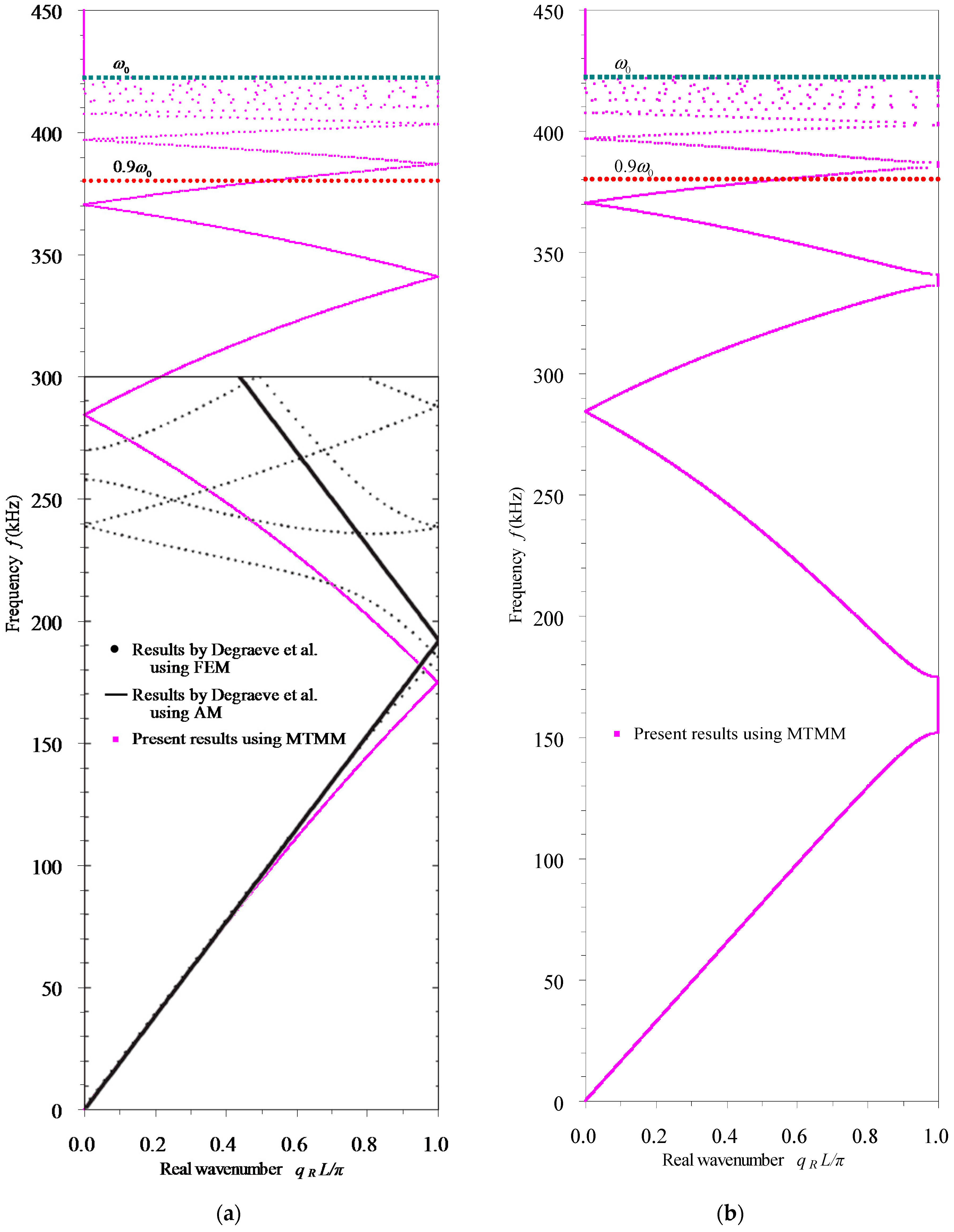
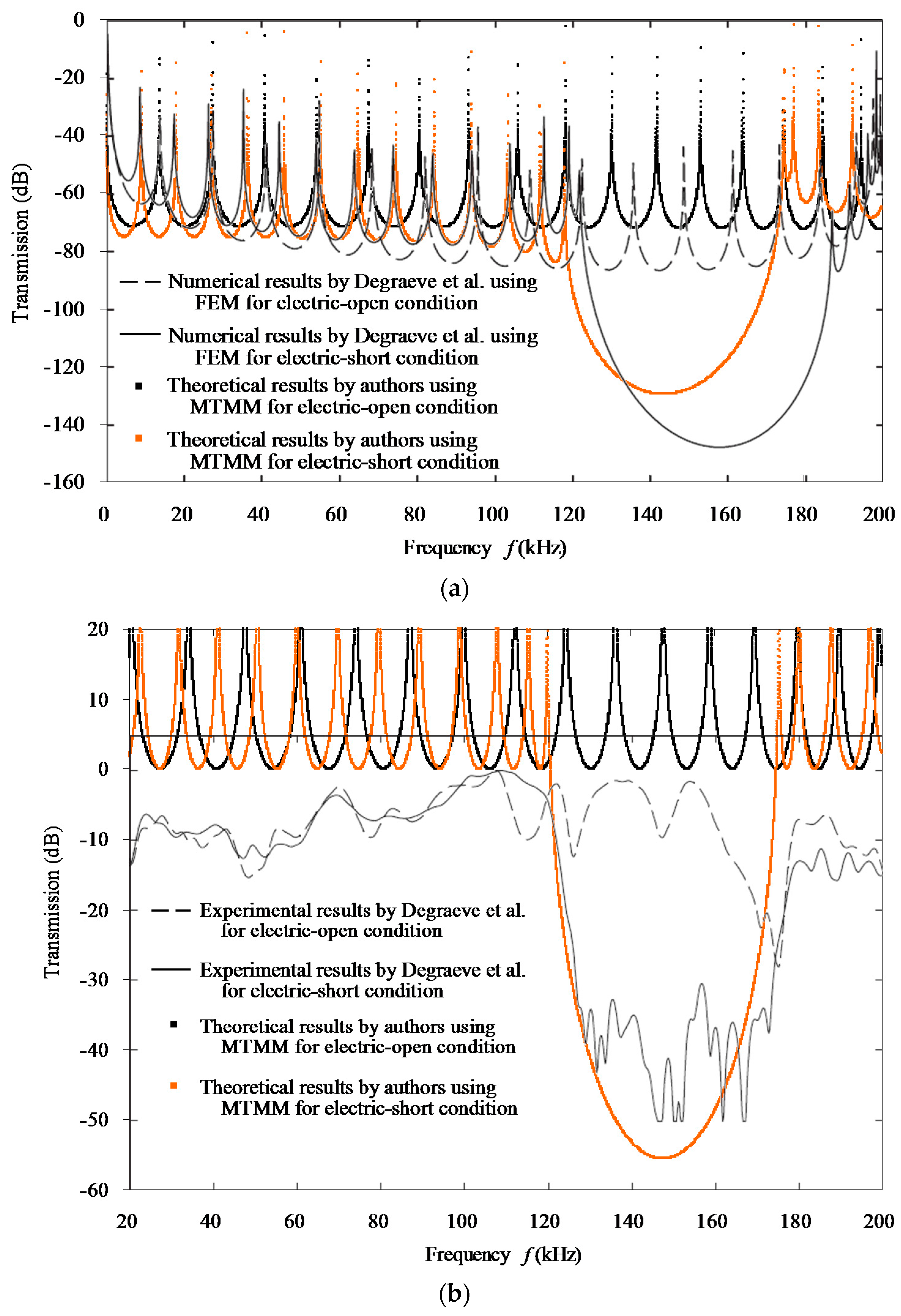
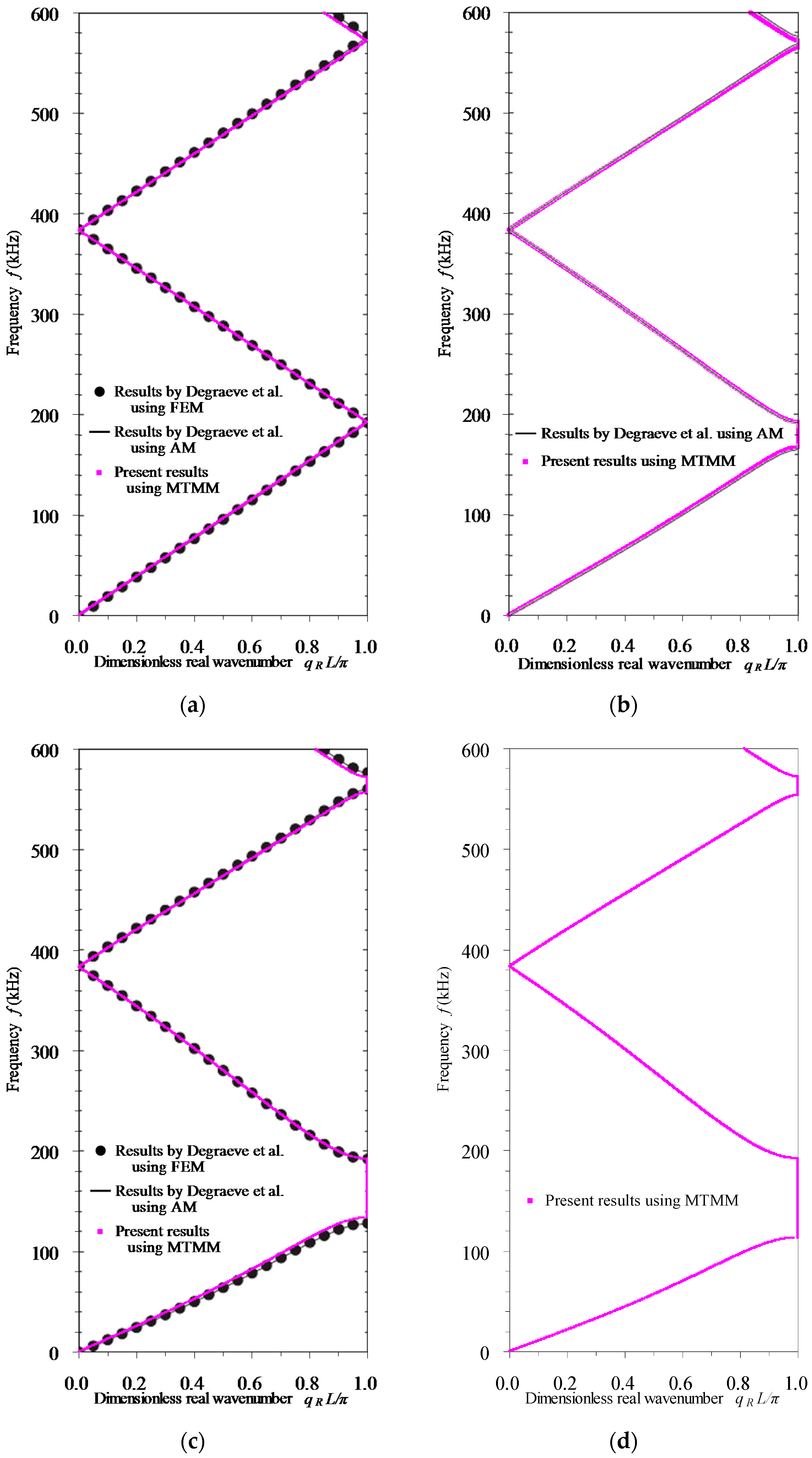
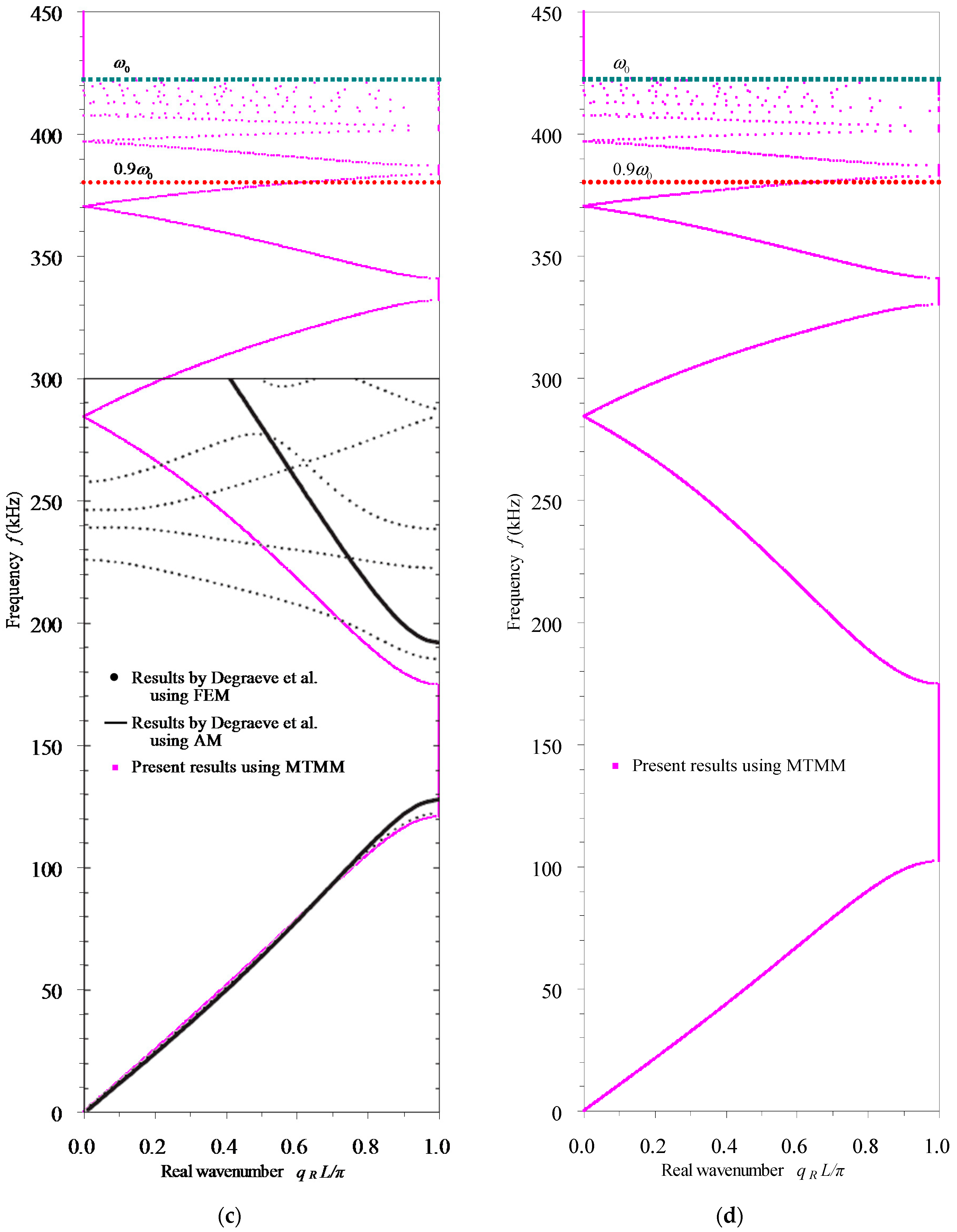
3.1. Validation of the Proposed MTMM

First, consider a periodic piezoelectric composite rod [20] consisting of alternate $10 \text{mm}$ long circular PZT-5H (PZ29) rod and $0.025 \text{mm}$ long circular brass electrode all with $1 \text{mm}$ diameters. The piezoelectric PZT-5H constituent rod is poled along the $X$ axis in positive direction. The material and geometrical parameters of the two constituent rods in the unit cell [35] (pp. 358–382) are listed in

Table 2. Material and geometrical parameters.

Materials	Stiffness Constants ($\text{GPa}$)
	$c_{11}$	$c_{22}$	$c_{33}$			$c_{12}$			$c_{13}$	$c_{23}$
PZT-5H	117.0	126.0	126.0			84.1			84.1	79.5
Brass	162.46	162.46	162.46			82.58			82.58	82.58
Epoxy	6.98	6.98	6.98			3.76			3.76	3.76
Materials	Poisson’s Ratios		Piezoelectric Constants ($\mathrm{C}/{\mathrm{m}}^2$)						Dielectric Constants ($\times {10}^{-9} \mathrm{F}/\mathrm{m}$)
	${\nu }_{12}$	${\nu }_{13}$	$e_{11}$		$e_{12}$		$e_{13}$		${\alpha }_{11}$
PZT-5H	0.41	0.41	23.3		−6.5		−6.5		13.02
Brass	0.337	0.337	—		—		—		—
Epoxy	0.35	0.35	—		—		—		—
Materials	Mass Density ($\text{kg}/{\mathrm{m}}^3$)		Length ($\text{mm}$)			Cross-Sectional Area ($\times \pi { \text{mm}}^2$)			Cross-Sectional Moments of Inertia ($\times \pi { \text{mm}}^4$)
	$\rho$		$l$			$A$			$I_y$	$I_z$
PZT-5H	7500		10			1/4			1/64	1/64
Brass	8320		0.025			1/4			1/64	1/64
Epoxy	1180		10			1/4			1/64	1/64

except those specified otherwise. Four kinds of electrical boundaries, i.e., the electric-open, applied electric capacity, electric-short and applied feedback control conditions, are considered to impose on the electrodes. In order to compare to the results by Degraeve et al. [20], we neglect the mechanical vibration and the thickness of the brass electrodes but retain its electrical function for calculating the phase constant spectra ($q_R(\omega )L$ curves) of this PZT-5H piezoelectric rod with periodic electrical boundaries in the low and high frequency ranges. The results are given in Figure 3. For the convenience of description, the engineering frequency $f=\omega /(2\pi )$ and the dimensionless wavenumber $qL/\pi$ are used hereafter. The results of the first three electric boundaries are also compared in Figure 3 with the corresponding ones by Degraeve et al. using the analytical method (AM) [20]. It should be noted that the applied electric capacity is specified as the clamped capacitance $C=\alpha A/l=1.02\times {10}^{-12} \mathrm{F}$, which is the same as that used in [20].

Figure 3a–c indicates that the phase constant spectra of the first three electrical boundaries in the low frequency range $f\le 500 \text{kHz}$ obtained by our proposed MTMM generally agree well with their counterparts by Degraeve et al. using AM [20]. Nevertheless, the discrepancy becomes observable in the relatively high frequency range $500 \text{kHz}<f\le 600 \text{kHz}$. This is because that in the AM by Degraeve et al. [20], the classical rod theory applicable to pretty low frequency range is adopted. Our proposed MTMM, which adopts the Love rod theory, is effective till to a relative high frequency $0.9{\omega }_0=3.81 \text{MHz}$ with ${\omega }_0=\min ({\omega }_C^{(1)},{\omega }_C^{(2)},\cdots ,{\omega }_C^{(m)})$ the minimum of critical frequencies of the constituent rods (For piezoelectric PZT-5H rod, ${\omega }_C=\sqrt{[(c+e^2/\alpha )A]/[\rho ({\nu }_{12}^2{I}_z+{\nu }_{13}^2{I}_y)]}=4.23 \text{MHz}$; For brass electrode, ${\omega }_C=\sqrt{cA/[\rho ({\nu }_{12}^2{I}_z+{\nu }_{13}^2{I}_y)]}=4.79 \text{MHz}$) [28]. Figure 3d shows that our proposed MTMM works also well for analyzing the phase constant spectra of the applied feedback control condition in the low frequency range. Figure 3a–d illustrates that, in any electric boundary case, the width of stop-bands decreases with its order. The comparisons of Figure 3a–d indicate that the widths of stop-bands become wider and the central frequencies of stop-bands become lower in sequence of electric-open (without band gaps), applied electric capacity, electric-short and applied feedback control boundaries due to the separate increasing of coefficient $B$. However, this difference between the band structures of the four electrical boundaries is inconspicuous in the high frequency range, as shown in Figure 3e, since the band gaps of the latter three electrical boundaries all become trivial in that frequency range. This is because the axial-force influence coefficient $B$ of the piezoelectric rod, which is relative to the electric boundary conditions, do not change with frequency. However, the axial-force influence coefficient ${\zeta }_1$, which is irrelative to the electric boundary conditions, obviously increases near linearly with the frequency $\omega$. In all the four periodically electrical boundary cases, since the $B$-${\zeta }_1$ ratio decreases very quickly with the increasing of frequency, the widths of band gaps determined by this ratio thus approach to zero quickly even the folding of bands is identifiable. The above results and the Figure 3e demonstrate that our proposed MTMM works very well in frequency range below $0.9{\omega }_0$ for all four kinds of electrical boundaries.

Second, consider the same periodic piezoelectric composite rod as above except that the diameters of all constituent rods are $10 \text{mm}$ [20] and the mechanical vibration of the brass electrodes is also reckoned in. The current minimum critical frequency of the constituent rods is ${\omega }_0=423 \text{kHz}$. Thus it has $0.9{\omega }_0=381 \text{kHz}$. Using our proposed MTMM, we calculate the phase constants spectra of this periodic PZT-5H piezoelectric rod covered by brass electrodes below $450 \text{kHz}$ for all the four electrical boundary conditions. Figure 4a–d provides the results associated with the electric-open, applied electric capacity, electric-short and applied feedback control conditions, respectively, in which the lines of ${\omega }_0$ and $0.9{\omega }_0$ are also depicted. In particular, the results of the electric-open and electric-short boundaries are compared with the corresponding ones by Degraeve et al. using the FEM and AM [20] in Figure 4a,c, respectively. In these two electrical boundary cases, the transmission spectra of a finite periodic piezoelectric composite rod consisting of 14 unit cells are also calculated by our MTMM, which are depicted and compared in Figure 5 with the corresponding results by Degraeve et al. [20]. In order to compare to the numerical transmission from FEM [20], the ordinate in Figure 5a is specified as $20{\log }_{10}\left\{\left|1/[(c+e^2/\alpha )A{T}_{G12}]\right|\right\}$, where the parameters of PZT-5H are utilized. In Figure 5b, the ordinate is the transmission $R$ computed from $T_{G22}$ by using Equation (25), for the sake of comparing with the experiment measurements [20].

In the electric-open and electric-short boundary cases, Figure 4a,c indicates that the phase constant spectra below $200 \text{kHz}$ from our proposed MTMM in general agree with both the results of FEM and those of AM by Degraeve et al. [20]. Figure 5a also shows that below $200 \text{kHz}$ the transmission spectra from our MTMM in general agree with the numerical transmission from FEM by Degraeve et al. [20]. The observable differences in these figures may be caused by that the FEM considers all modes and their coupling, while our MTMM considers only the longitudinal mode but with taking the Poisson’s effect into account. These differences are also due to that the vibration of electrodes is not taken into account in the FEM (and AM) models by Degraeve et al. [20]. Figure 5b manifests clearly that our predicated transmission spectra in the stop bands agree very well with the measured transmission. However, in the pass bands, our MTMM results are about 20 dB bigger than the experimental results. The damping in the experimental specimen may be the primary cause. Figure 4c and Figure 5 also indicate that the first stop bands of the model with electric-short boundary condition predicated by the phase constant spectra and by the transmission spectra are coincident. In the range of $200 \text{kHz}<f\le 300 \text{kHz}$, the phase constant spectra from our proposed MTMM give better prediction to those of FEM than the results of AM. The reason is that our proposed MTMM considers the Poisson’s effect while the AM neglects it. The deviation between our MTMM results and those from FEM may be due to two reasons. One is that the FEM considers all modes and their coupling, while our MTMM considers only the longitudinal mode with considering the Poisson’s effect. The other is that the electrode vibration is ignored in the FEM model. In all the four electrical boundary cases, our MTMM works well till to the frequency $0.9{\omega }_0=381 \text{kHz}$ with ${\omega }_0=423 \text{kHz}$ the minimum critical frequency of the constituent rods. In the higher frequency range, the proposed MTMM loss efficacy since the Love rod theory becomes invalid. In sequence of electric-open, applied electric capacity, electric-short and applied feedback control boundaries, the increasing of stop-band widths and the reduction of the stop-band central frequencies still hold due to the separate increasing of coefficient $B$.

3.2. Passive Control of Longitudinal Waves in Rod-Type Piezoelectric Phononic Crystals

Consider the same rod-type piezoelectric phononic crystal with $1 \text{mm}$ diameters as in Section 3.1, but now reckon in the mechanical vibration of the brass electrodes. The electrode’s thickness, the rod’s cross-sectional dimension and the elastic rod insert are individually varied to show their influences on the band structures, while the other parameters remain the same as in Table 2.

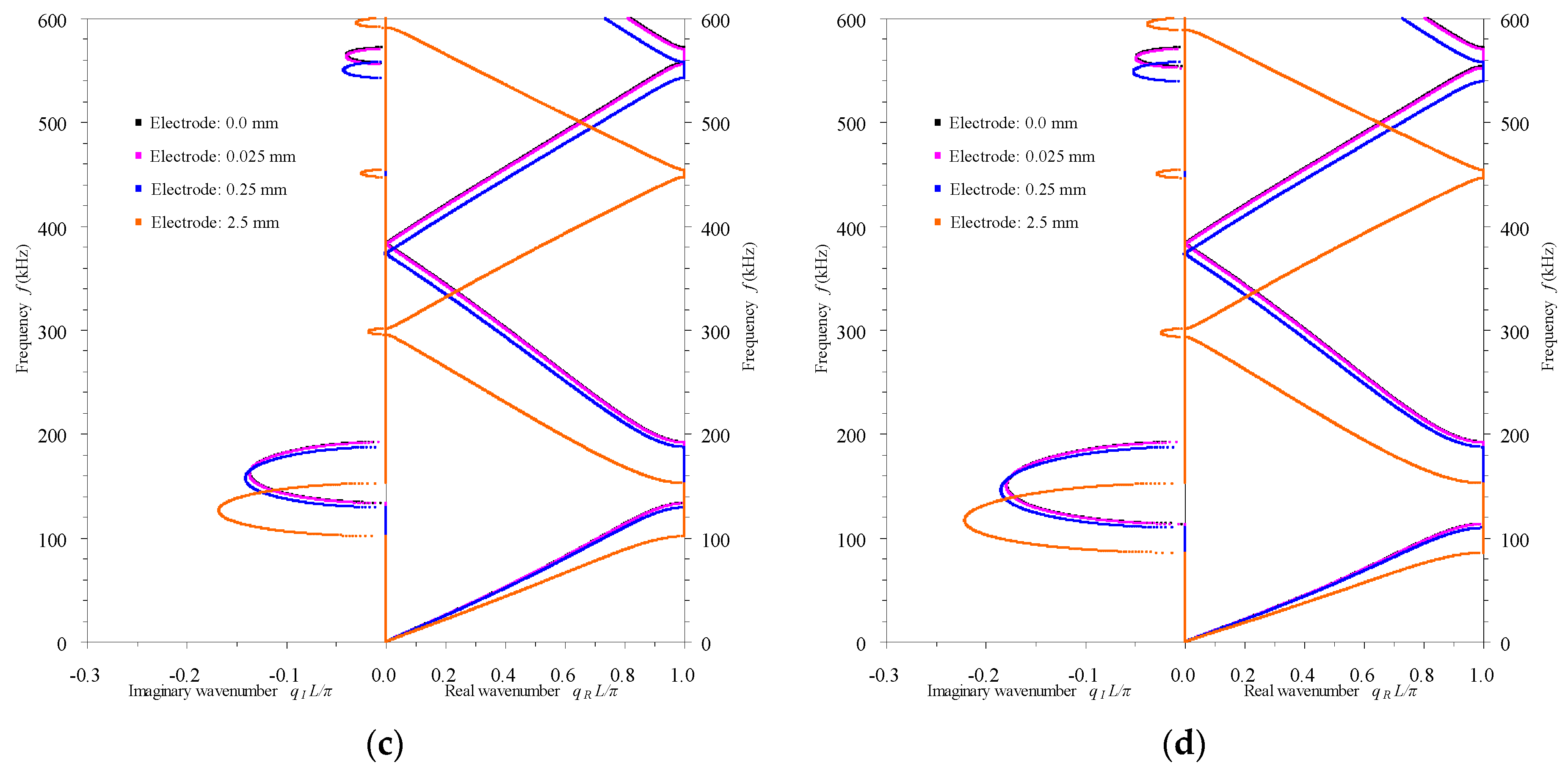
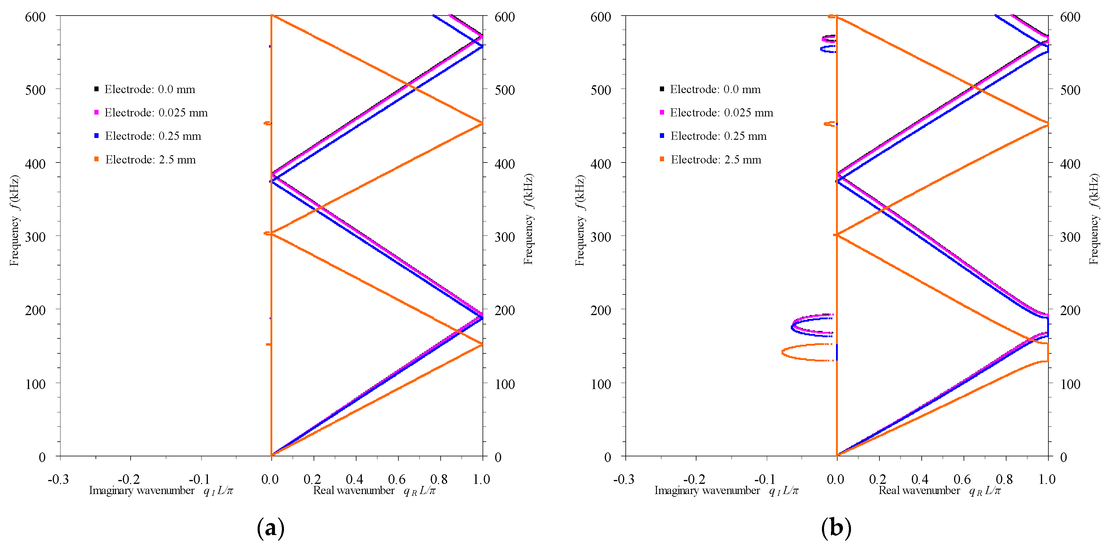
3.2.1. Influence of the Electrode’s Thickness

Specifying the thickness of the electrode as $0.025 \text{mm}$, $0.25 \text{mm}$ and $2.5 \text{mm}$, we calculate the propagation constants spectra including the phase constant spectra and the attenuation constant spectra ($q_I(\omega )L$ curves) of the periodic PZT-5H piezoelectric rod covered by brass electrodes with the four periodic electrical boundaries, respectively, and compare them with those results as the electrode’s thickness is neglected, as given in Figure 6.

Figure 6 illustrates that with an increase in the electrode’s thickness, the central frequencies of all the stop-bands and the width of the first stop-band slightly decrease, although this feature is not apparently clear as the electrode’s thickness varies from $0$ to $0.025 \text{mm}$. The maximum value of attenuation constants in the first stop-band increases with the electrode’s thickness.

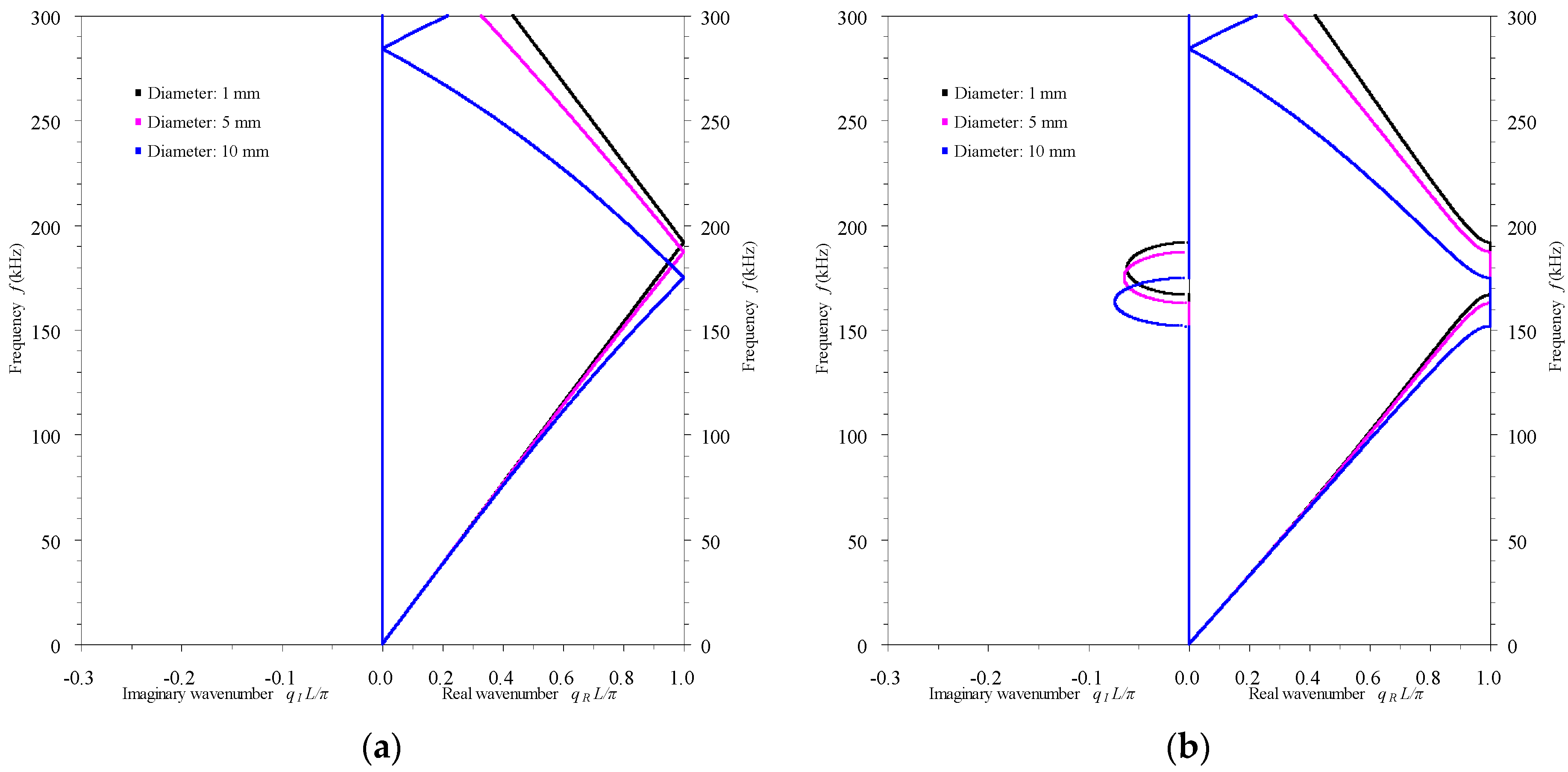
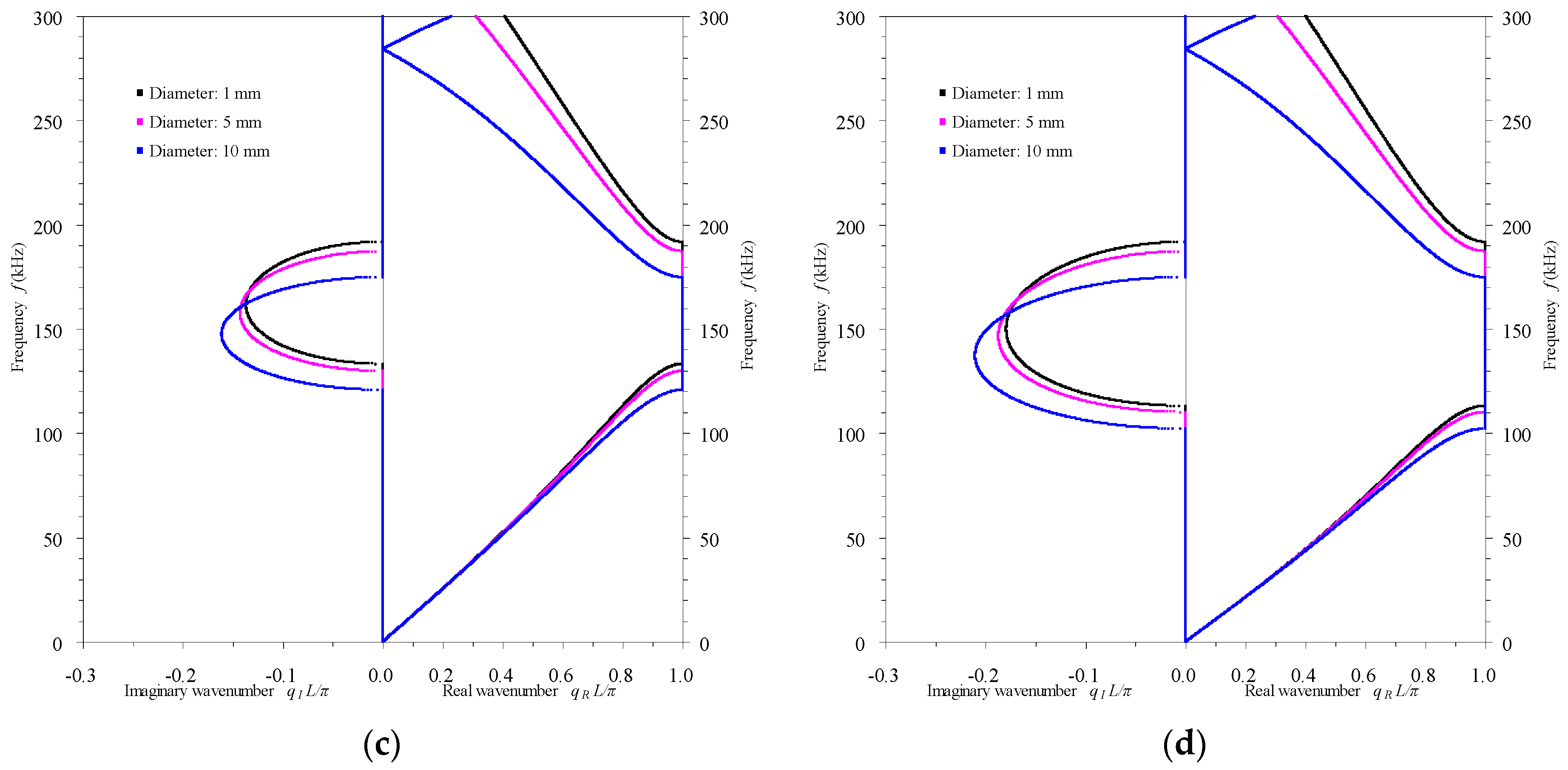
3.2.2. Influence of the Rod’s Cross-Sectional Dimension

As the diameter of all the constituent rods is $1 \text{mm}$, $5 \text{mm}$ and $10 \text{mm}$, respectively, the propagation constants spectra of the periodic PZT-5H piezoelectric rod covered by brass electrodes are calculated by our proposed MTMM. Figure 7a–d provides the results associated with the electric-open, applied electric capacity, electric-short and applied feedback control conditions, respectively.

Figure 7a–d indicates that, in any electrical boundary case, the central frequencies of all the stop-bands decrease and the maximum attenuation constant in the first stop-band slightly increase with an increase in the rods’ diameter. These phenomena reflect the influence of the Poisson’s effect on the band structures. The bigger the rods’ diameter is, the larger the Poisson’s effect.

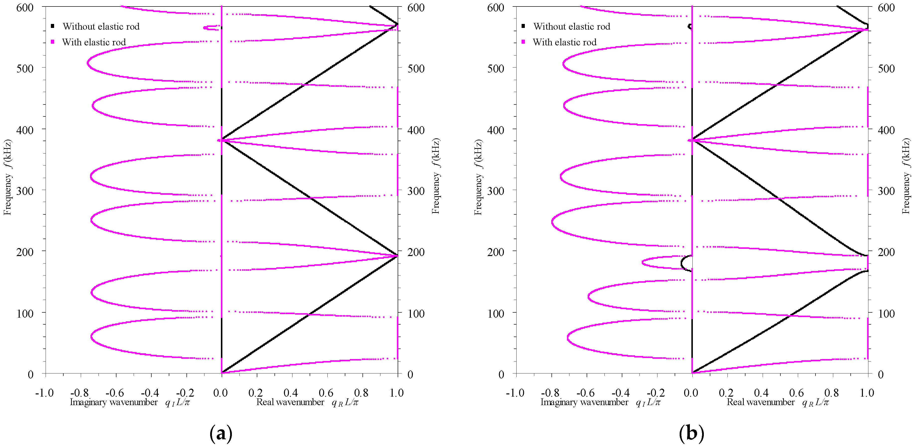
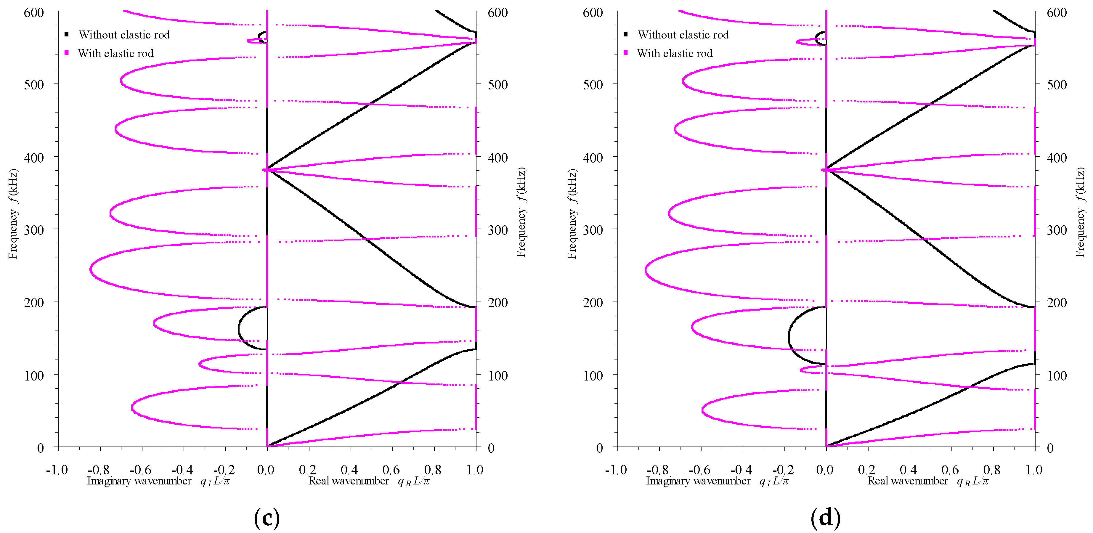
3.2.3. Influence of the Elastic Rod Insert

As an elastic rod made of epoxy, whose material and geometrical parameters are given in Table 2, is inserted into the unit cell of the periodic PZT-5H piezoelectric rod covered by brass electrodes, the propagation constants spectra are computed and compared with the results of the periodic composite rod without the epoxy component in unit cell, as depicted in Figure 8a–d in the four electrical boundary cases, respectively.

Figure 8a–d shows that inserting an elastic rod in unit cell adds many new band structures in all the four electrical boundary cases, which is due to the interaction between the elastic and piezoelectric constituent rods. When an elastic rod is inserted into the unit cell, the differences between band structures associated with the four electrical conditions are weakened. Since the inserted elastic rod is softer than the original piezoelectric rod, the values of the attenuation constants enormously enlarge. In the latter three electrical conditions, after the epoxy rod is inserted in the unit cell, the original first stop-band turns into the third stop-band, with the central frequency increased slightly and the width decreased.

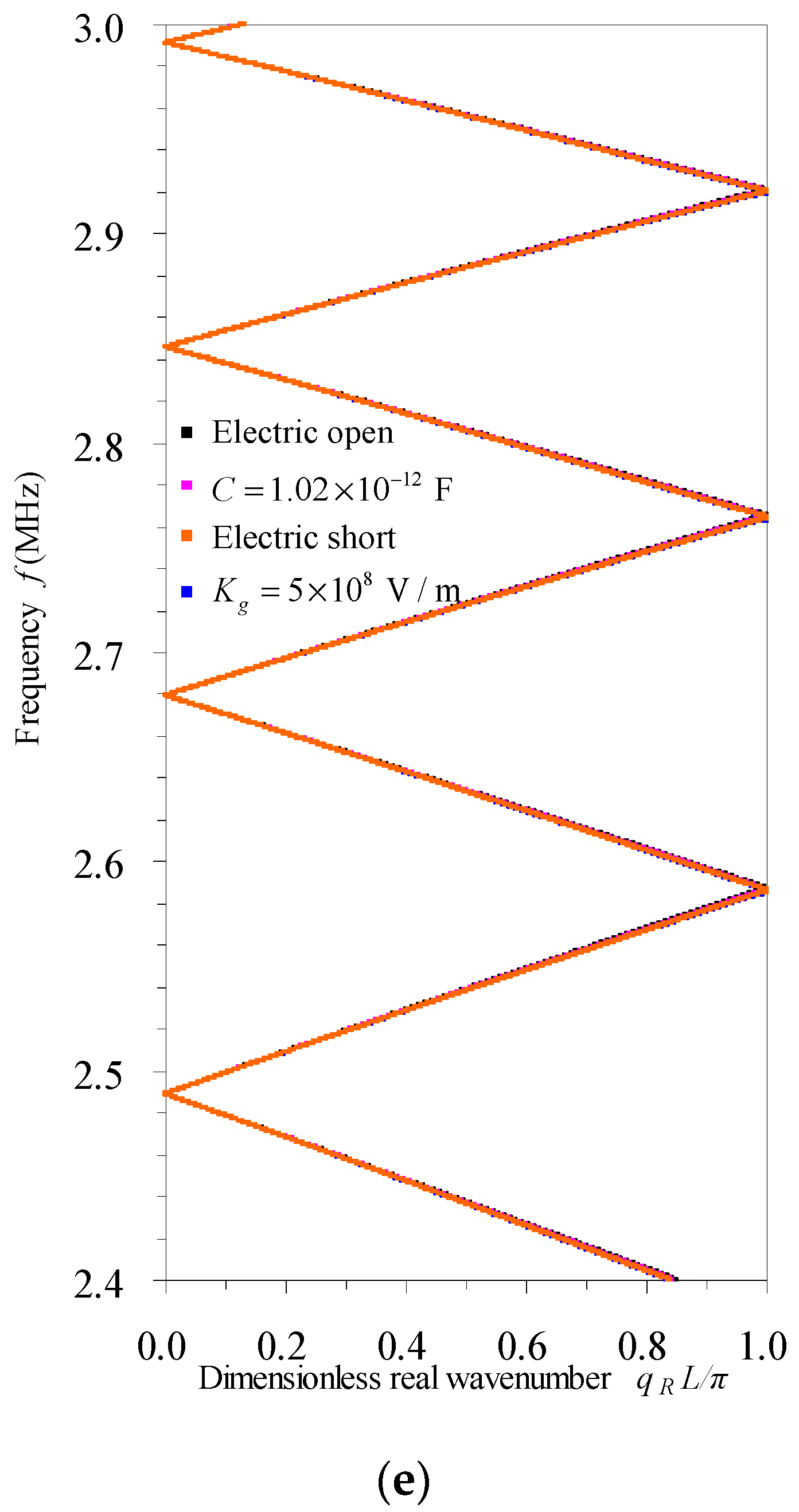
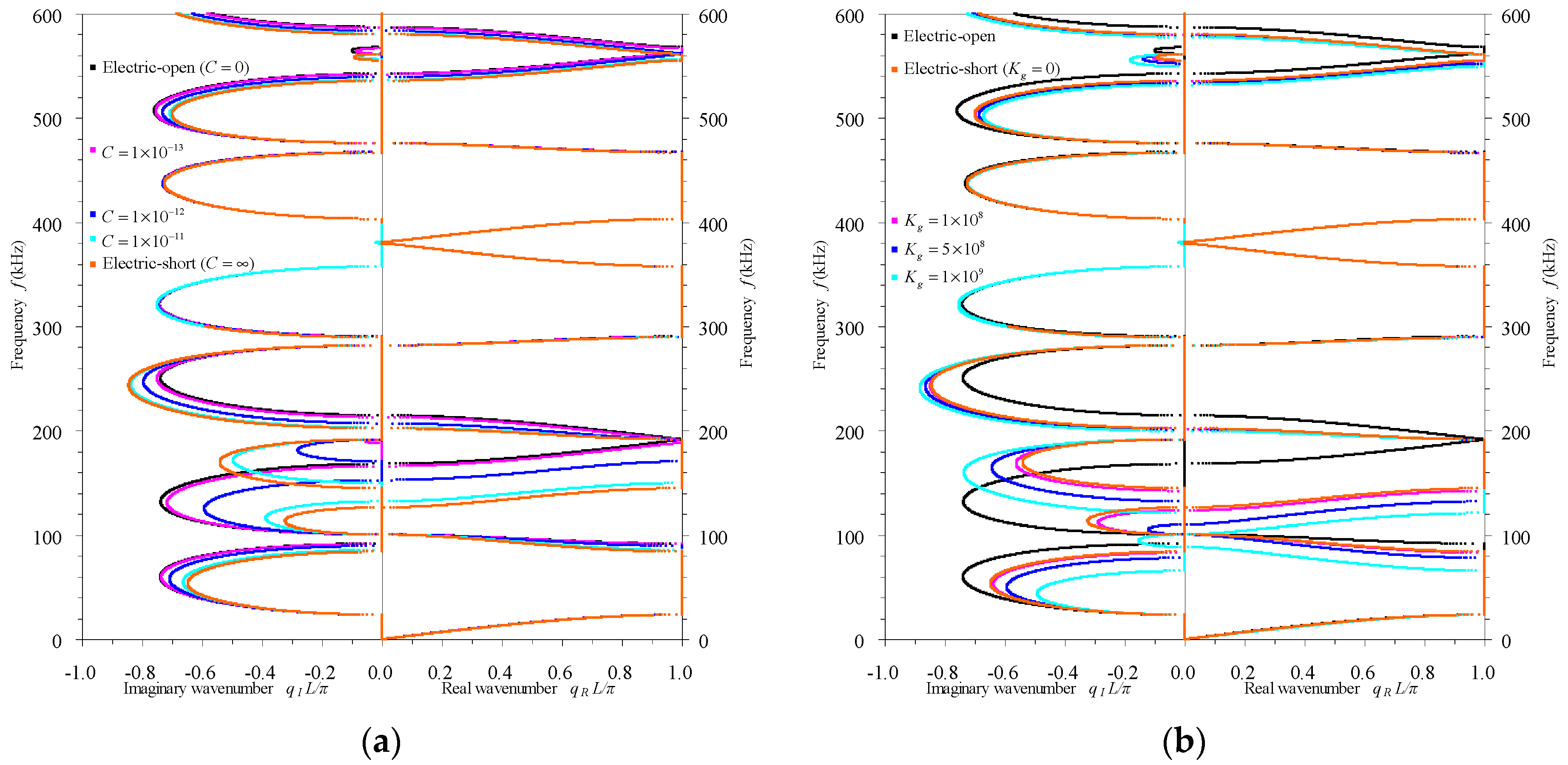
3.3. Active Control of Longitudinal Waves in Rod-Type Piezoelectric Phononic Crystals

Consider the same rod-type piezoelectric phononic crystal as studied in Section 3.2.3. Its unit cell, as referred to in Figure 1, is composed of an epoxy elastic rod, a brass electrode, a PZT-5H piezoelectric rod and a brass electrode. Their material and geometrical parameters are listed in Table 2. On the electrodes, external electric capacitor and feedback controller are connected to investigate the influences of applied electric capacity and feedback control boundaries on the band structures, respectively.

First, specifying the applied electric capacitance as $C=1\times {10}^{-13} \mathrm{F}$, $C=1\times {10}^{-12} \mathrm{F}$ and $C=1\times {10}^{-11} \mathrm{F}$, individually, we compute the propagation constants spectra of the periodic Epoxy-Brass-PZT-5H-Brass composite rod to study the influence of applied electric capacity on the band structures. The results are given in Figure 9a, where they are compared with those of the electric-open ($C=0$) and the electric-short ($C=\infty$) boundary conditions. Second, when the applied feedback control is specified by the control gain as $K_g=1\times {10}^8 \mathrm{V}/\mathrm{m}$, $K_g=5\times {10}^8 \mathrm{V}/\mathrm{m}$ and $K_g=1\times {10}^9 \mathrm{V}/\mathrm{m}$, respectively, the propagation constants spectra of the periodic Epoxy-Brass-PZT-5H-Brass composite rod are calculated to discuss the influence of applied feedback control on the band structures. The results are depicted and compared with those of the electric-open and the electric-short ($K_g=0$) boundary conditions in Figure 9b.

Figure 9a indicates that when the applied electric capacity is increased from 0 to infinity, the spectra of the propagation constants, as expected, change gradually from those of the electric-open condition to those of the electric-short condition. New stop-bands may first appear, and then most of the propagation constants spectra alter towards the frequency reducing direction. Thus, the central frequencies of these stop-bands and pass-bands decrease obviously with an increase in the electric capacitance. However, some band structures in certain frequency ranges, 0 – 40 kHz and 270 – 490 kHz in Figure 9a, do not alter with the applied electric capacitance, which are probably formed due mainly to the mechanical effect of the periodic composite rod. Note from Figure 9b that with the increasing of control gain from $0$, the propagation constants spectra change from those of the electric-short condition towards the frequency reducing direction. The central frequencies of most stop-bands and pass-bands decrease obviously with an increase in the control gain. However, the band structures in the same frequency ranges (0 – 40 kHz and 270 – 490 kHz) as in Figure 9a, do not change at all. This again testifies that these band structures have nothing to do with the electrical boundaries.

If the influence of the electrical boundaries on the band structures is overall considered when comparing Figure 9a with Figure 9b, it can be concluded that the band structures of the electric-short condition play a referential role. The band structures of the applied electric capacity $C$ (and electric-open $C=0$) condition lie on their lower-frequency side, while those of the applied feedback control with control gain $K_g$ locate on their higher-frequency side. Consequently, in the following we focus on the electric-short condition to discuss the dispersion properties of the characteristic longitudinal waves in the rod-type piezoelectric phononic crystals.

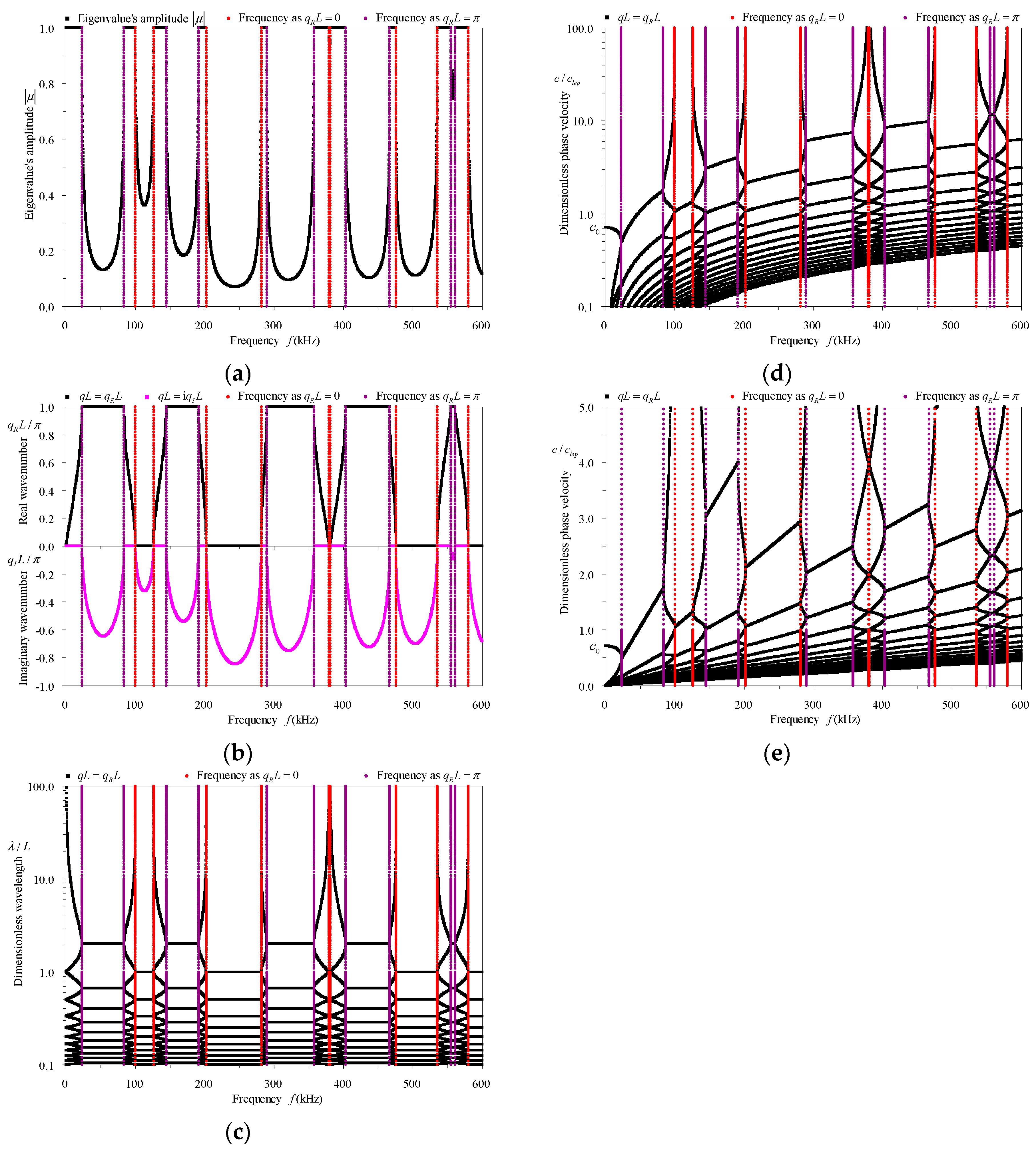
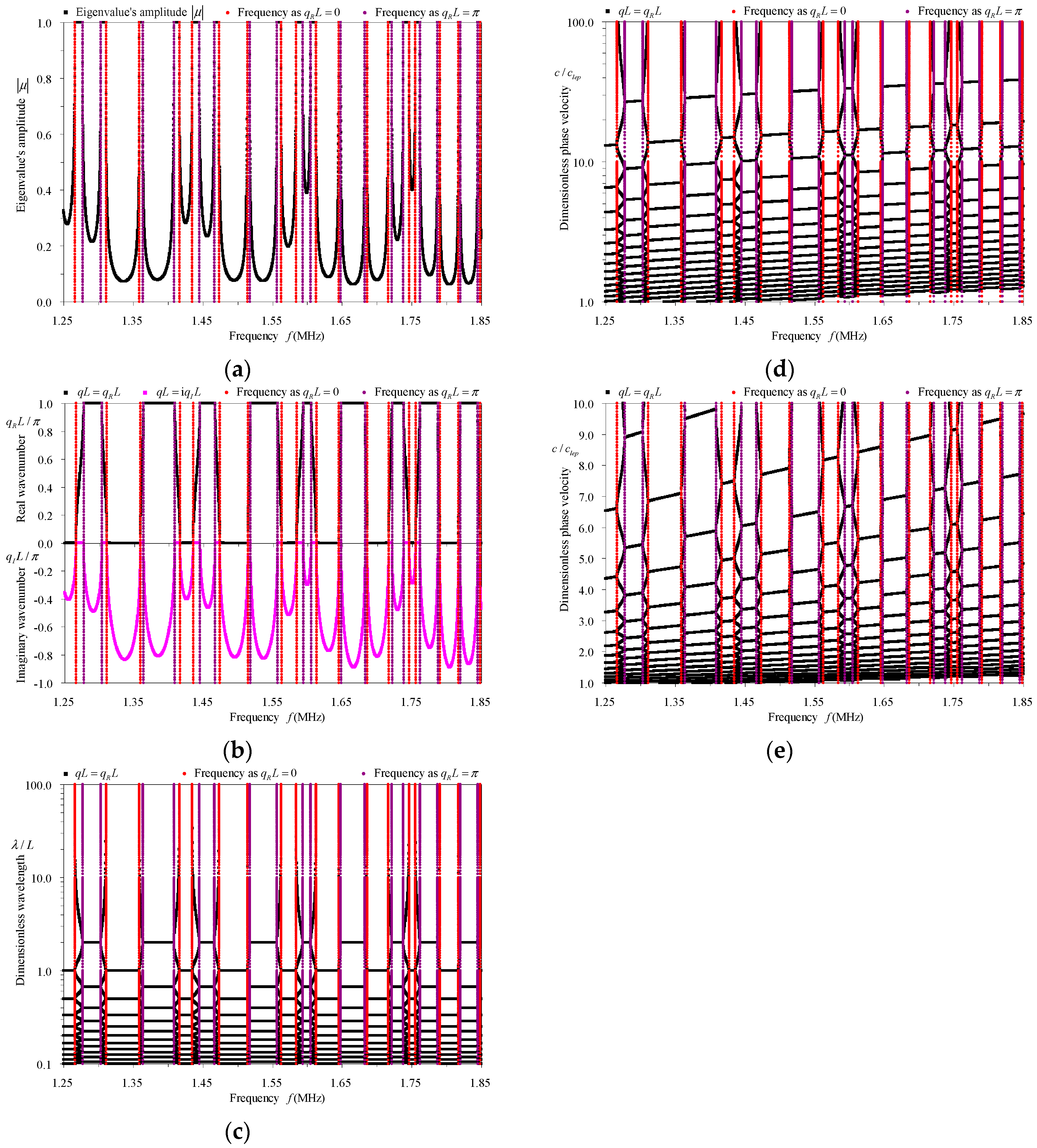
3.4. Dispersion Properties of Longitudinal Waves in Rod-Type Piezoelectric Phononic Crystals

In the case of electric-short boundary condition, comprehensive frequency-related dispersion curves, which include the eigenvalue’s amplitude spectra ($\left|\mu \right|(\omega )$ curves), the wavenumber spectra ($q(\omega )$ curves), the wavelength spectra ($\lambda (\omega )$ curves), the phase velocity spectra ($c(\omega )$ curves), of the above discussed periodic Epoxy-Brass-PZT-5H-Brass composite rod are calculated in both low ($f\le 600 \text{kHz}$) and high ($1.25 \text{MHz}\le f\le 1.85 \text{MHz}$) frequency ranges. Please notice that the minimum critical frequency is ${\omega }_0={\omega }_C^{(Epoxy)}=2.47 \text{MHz}$. Thus, our MTMM is valid till to $0.9{\omega }_0=2.22 \text{MHz}$. The low and high frequency results are provided in Figure 10 and Figure 11, respectively. For the convenience of presentation, the dimensionless wavelength $\lambda /L$ and phase velocity $c/c_{lep}$ are further introduced except for the engineering frequency $f=\omega /(2\pi )$ and the dimensionless wavenumber $qL/\pi$. $c_{lep}=\sqrt{c_{ep}/{\rho }_{ep}}$ is the longitudinal wave speed in the epoxy rod without considering the Poisson’s effect, where $c_{ep}=E_{ep}$ and ${\rho }_{ep}$ are the Young’s modulus and the material density of epoxy, respectively.

Figure 10a–e and Figure 11a–e reflect that, in addition to the same dispersion properties of longitudinal waves in general periodic rods [5,37], the characteristic longitudinal waves in a rod-type piezoelectric phononic crystal also possess the following dispersion properties:

(1)

The eigenvalue’s amplitude spectra, which cannot be obtained by MRRM [5], demonstrate clearly the width, the central frequencies and the bounding frequencies of the pass-bands ($\left|\mu \right|=1$) and the stop-bands ($\left|\mu \right|\ne 1$). They also reflect the attenuation amplitudes ${\mathrm{e}}^{q_{I}L}$ of waves in the stop-bands, which are verified by the attenuation constant ($q_{I}L$) spectra. The eigenvalue’s amplitude spectra cannot indicate the properties of waves in the pass-bands, but the phase constant spectra do.

(2)

In these frequency-related dispersion curves, the bounding frequencies of the odd and even order stop-bands correspond to $qL=q_{R}L=(2n+1)\pi$ and $qL=q_{R}L=2n\pi$ ($n$ is a natural number), respectively. Within the stop-bands, the real part ($q_{R}L$) of the complex wavenumber $qL$, which cannot be computed by the MRRM [5] but obtained here by the MTMM, have the same phases as their boundaries. In the wavelength spectra, the representations corresponding to these two kinds of phases are horizontal lines $\lambda /L=2/(2n+1)$ and $\lambda /L=1/n$. In the phase velocity spectra, they correspond to inclined lines that pass through the origin and have slopes $c/\omega =L/[(2n+1)\pi ]$ $c/\omega =L/[2n\pi ]$, respectively. The lines determined by the above formulas and the lines of bounding frequencies form the grids to draw the spectra in the corresponding frequency-related dispersion curves.

4. Conclusions

A modified transfer matrix method (MTMM), which is based on the Love rod theory and the method of reverberation-ray matrix (MRRM), is proposed in this paper for the analysis of characteristic longitudinal waves by combining Floquet–Bloch principle and for the calculation of transmission spectra in general rod-type piezoelectric phononic crystals with electric-open, applied electric capacity, electric-short and applied feedback control conditions. Numerical examples are given to validate the proposed MTMM, to study the passive control of the band structures by the electrode’s thickness, the rod’s cross-sectional dimension and the elastic rod insert, and to investigate the active tuning of the band structures by the electrical boundary conditions. The dispersion properties are summarized from the comprehensive frequency spectra. From these analyses, we can draw the conclusions as follows:

(1)

The proposed analytical MTMM provides an alternative analysis method for the complex band structures and transmission spectra till to $0.9{\omega }_0$ (${\omega }_0$ is the minimum critical frequency) within which the Love rod theory is valid. Its effectiveness is validated by some numerical examples.

(2)

In passive mode, the electrode’s thickness and the rod’s cross-sectional dimension can be used to slightly adjust the band structures of the rod-type piezoelectric phononic crystals, while the elastic rod insert is able to enormously alter the band structures.

(3)

In active mode, the switchable electrical boundaries among electric-short, applied electric capacity, electric-open and applied feedback control conditions is effective for modulating some of the band structures that are related to the electromechanical coupling of the rod-type piezoelectric phononic crystals. The tunable capacity and control gain in the applied electric capacity and applied feedback control cases, respectively, can also be used for tuning the propagation of longitudinal waves. The band structures of the electric-short condition play a referential role for designing the active control scheme.

References

1. Kushwaha, M.S.; Halevi, P.; Dobrzynski, L.; Djafari-Rouhani, B. Acoustic band structure of periodic elastic composites. Phys. Rev. Lett. 1993, 71, 2022–2025. [Google Scholar] [CrossRef] [PubMed]
2. Deymier, P.A. (Ed.) Acoustic Metamaterials and Phononic Crystals; Springer: Berlin, Germany, 2013.
3. Asiri, S.; Baz, A.; Pines, D. Periodic struts for gearbox support system. J. Vib. Control 2005, 11, 709–721. [Google Scholar] [CrossRef]
4. Asiri, S. Vibration isolation of automotive vehicle engine using periodic mounting systems. Proc. SPIE 2005, 5760, 526–537. [Google Scholar]
5. Guo, Y.Q.; Fang, D.N. Analysis and interpretation of longitudinal waves in periodic multiphase rods using the method of reverberation-ray matrix combined with the Floquet-Bloch theorem. ASME J. Vib. Acoust. 2014, 136, 011006. [Google Scholar] [CrossRef]
6. Ruzzene, M.; Baz, A. Attenuation and localization of wave propagation in periodic rods using shape memory inserts. Smart Mater. Struct. 2000, 9, 805–816. [Google Scholar] [CrossRef]
7. Ruzzene, M.; Baz, A. Control of wave propagation in periodic composite rods using shape memory inserts. ASME J. Vib. Acoust. 2000, 122, 151–159. [Google Scholar] [CrossRef]
8. Ding, R.; Su, X.L.; Zhang, J.J.; Gao, Y.W. Tunability of longitudinal wave band gaps in one dimensional phononic crystal with magnetostrictive material. J. Appl. Phys. 2014, 115, 074104. [Google Scholar] [CrossRef]
9. Baz, A. Active control of periodic structures. ASME J. Vib. Acoust. 2001, 123, 472–479. [Google Scholar] [CrossRef]
10. Thorp, O.; Ruzzene, M.; Baz, A. Attenuation and localization of wave propagation in rods with periodic shunted piezoelectric patches. Smart Mater. Struct. 2001, 10, 979–989. [Google Scholar] [CrossRef]
11. Chen, S.B.; Wen, J.H.; Wang, G.; Yu, D.L.; Wen, X.S. Improved modeling of rods with periodic arrays of shunted piezoelectric patches. J. Intell. Mater. Syst. Struct. 2012, 23, 1613–1621. [Google Scholar]
12. Lossouarn, B.; Aucejo, M.; Deu, J.-F. Multimodal coupling of periodic lattices and application to rod vibration damping with a piezoelectric network. Smart Mater. Struct. 2015, 24, 045018. [Google Scholar] [CrossRef]
13. Lossouarn, B.; Aucejo, M.; Deu, J.-F. Multimodal vibration damping through a periodic array of piezoelectric patches connected to a passive network. Proc. SPIE 2015, 9431, 94311A. [Google Scholar]
14. Singh, A.; Pines, D.J.; Baz, A. Active/passive reduction of vibration of periodic one-dimensional structures using piezoelectric actuators. Smart Mater. Struct. 2004, 13, 698–711. [Google Scholar] [CrossRef]
15. Asiri, S.; Baz, A.; Pines, D. Active periodic struts for a gearbox support system. Smart Mater. Struct. 2006, 15, 1707–1714. [Google Scholar] [CrossRef]
16. Asiri, S. Tunable mechanical filter for longitudinal vibrations. Shock Vib. 2007, 14, 377–391. [Google Scholar] [CrossRef]
17. Asiri, S. Broadband vibration attenuation using hybrid periodic rods. J. Eng. Res. 2008, 5, 7–19. [Google Scholar]
18. Li, F.M.; Wang, Y.S.; Chen, A.L. Wave localization in randomly disordered periodic piezoelectric rods. Acta Mech. Solida Sin. 2006, 19, 50–57. [Google Scholar]
19. Wang, Y.Z.; Li, F.M.; Kishimoto, K.; Wang, Y.S.; Huang, W.H. Wave localization in randomly disordered periodic piezoelectric rods with initial stress. Acta Mech. Solida Sin. 2008, 21, 529–535. [Google Scholar] [CrossRef]
20. Degraeve, S.; Granger, C.; Dubus, B.; Vasseur, J.O.; Thi, M.P.; Hladky-Hennion, A.-C. Bragg band gaps tunability in an homogeneous piezoelectric rod with periodic electrical boundary conditions. J. Appl. Phys. 2014, 115, 194508. [Google Scholar] [CrossRef]
21. Kutsenko, A.A.; Shuvalov, A.L.; Poncelet, O.; Darinskii, A.N. Quasistatic stopband and other unusual features of the spectrum of a one-dimensional piezoelectric phononic crystal controlled by negative capacitance. C. R. Mec. 2015, 343, 680–688. [Google Scholar] [CrossRef]
22. Ponge, M.-F.; Dubus, B.; Granger, C.; Vasseur, J.O.; Thi, M.P.; Hladky-Hennion, A.-C. Theoretical and experimental analyses of tunable Fabry-Perot resonators using piezoelectric phononic crystals. IEEE Trans. Ultrason. Ferroelectr. Freq. Control 2015, 62, 1114–1121. [Google Scholar] [CrossRef] [PubMed]
23. Degraeve, S.; Granger, C.; Dubus, B.; Vasseur, J.O.; Thi, M.P.; Hladky, A.C. Tunability of Bragg band gaps in one-dimensional piezoelectric phononic crystals using external capacitances. Smart Mater. Struct. 2015, 24, 085013. [Google Scholar] [CrossRef]
24. Degraeve, S.; Granger, C.; Dubus, B.; Vasseur, J.O.; Thi, M.P.; Hladky-Hennion, A.-C. Tunability of a one-dimensional elastic/piezoelectric phononic crystal using external capacitances. Acta Acust. United Acust. 2015, 101, 494–501. [Google Scholar] [CrossRef]
25. Kutsenko, A.A.; Shuvalov, A.L.; Poncelet, O.; Darinskii, A.N. Tunable effective constants of the one-dimensional piezoelectric phononic crystal with internal connected electrodes. J. Acoust. Soc. Am. 2015, 137, 606–616. [Google Scholar] [CrossRef] [PubMed]
26. Vasilenko, A.V.; Rogacheva, N.N. The effective characteristics and electroelastic state of active composite elements. PMM-J. Appl. Math. Mech. 2011, 75, 463–471. [Google Scholar] [CrossRef]
27. Love, A.E.H. A Treatise on the Mathematical Theory of Elasticity, 4th ed.; Cambridge University Press: Cambridge, UK, 1927; p. 428. [Google Scholar]
28. Graff, K.F. Wave Motion in Elastic Solids; Ohio State University Press: Columbus, OH, USA, 1975; pp. 108–125. [Google Scholar]
29. Doyle, J.F. Wave Propagation in Structures, 2nd ed.; Springer: New York, NY, USA, 1997. [Google Scholar]
30. Ravindra, B. Love-theoretical analysis of periodic system of rods. J. Acoust. Soc. Am. 1999, 106, 1183–1186. [Google Scholar] [CrossRef] [PubMed]
31. Brillouin, L. Wave Propagation in Periodic Structures: Electric Filters and Crystal Lattices, 2nd ed.; Dover Publications: New York, NY, USA, 1953. [Google Scholar]
32. Mead, D.J. Wave propagation in continuous periodic structures: Research contributions from Southampton, 1964–1995. J. Sound Vib. 1996, 190, 495–524. [Google Scholar] [CrossRef]
33. ANSI/IEEE Std 176-1987. IEEE Standard on Piezoelectricity; IEEE: New York, NY, USA, 1988; pp. 6–8. [Google Scholar]
34. Tiersten, H.F. Linear Piezoelectric Plate Vibrations; Plenum Press: New York, NY, USA, 1969; pp. 41–50. [Google Scholar]
35. Auld, B.A. Acoustic Fields and Waves in Solids; John Wiley & Sons: New York, NY, USA, 1973; Volume I. [Google Scholar]
36. Bronshtein, I.N.; Semendyayev, K.A.; Musiol, G.; Muehlig, H. Handbook of Mathematics, 5th ed.; Springer: Berlin, Germany, 2007. [Google Scholar]
37. Mead, D.J. Wave propagation and natural modes in periodic systems: I. Mono-coupled systems. J. Sound Vib. 1975, 40, 1–18. [Google Scholar] [CrossRef]
Figure 1. The unit cell of general periodic piezoelectric rods.
Crystals 06 00045 g001
Figure 2. The description of the unit cell: (a) the global and local coordinates; (b) the convention of generalized displacements and forces; and (c) the convention of wave amplitudes.
Crystals 06 00045 g002
Figure 3. The phase constant spectra of the homogeneous PZT-5H piezoelectric rod with periodic electrical boundaries: (a) electric-open condition; (b) applied electric capacity condition with C = α A / l = 1.02 × 10 12  F ; (c) electric-short condition; (d) applied feedback control condition with K g = 5 × 10 8  V / m ; and (e) all of the four abovementioned conditions in high frequency range.
Crystals 06 00045 g003aCrystals 06 00045 g003b
Figure 4. The phase constant spectra of the periodic PZT-5H piezoelectric rod covered by brass electrodes with periodic electrical boundaries: (a) electric-open condition; (b) applied electric capacity condition with C = α A / l = 1.02 × 10 10  F ; (c) electric-short condition; and (d) applied feedback control condition with K g = 5 × 10 8  V / m .
Crystals 06 00045 g004aCrystals 06 00045 g004b
Figure 5. The transmission (in dB units) in a finite periodic PZT-5H piezoelectric rod covered by brass electrodes consisting of 14 unit cells with electric-open and electric-short boundaries from our MTMM and their comparison with the corresponding ones by Degraeve et al. [20]: (a) comparison with the numerical transmission; and (b) comparison with the experimental transmission.
Crystals 06 00045 g005
Figure 6. Influence of the electrode’s thickness on the propagation constants spectra of the periodic PZT-5H piezoelectric rod covered by brass electrodes with periodic electrical boundaries: (a) electric-open condition; (b) applied electric capacity condition with C = α A / l = 1.02 × 10 12  F ; (c) electric-short condition; and (d) applied feedback control condition with K g = 5 × 10 8  V / m .
Crystals 06 00045 g006aCrystals 06 00045 g006b
Figure 7. Influence of the rod’s cross-sectional dimension on the propagation constants spectra of the periodic PZT-5H piezoelectric rod covered by brass electrodes with periodic electrical boundaries: (a) electric-open condition; (b) applied electric capacity condition with C = α A / l ; (c) electric-short condition; and (d) applied feedback control condition with K g = 5 × 10 8  V / m .
Crystals 06 00045 g007aCrystals 06 00045 g007b
Figure 8. Influence of the elastic rod insert on the propagation constants spectra of the periodic PZT-5H piezoelectric rod covered by brass electrodes with periodic electrical boundaries: (a) electric-open condition; (b) applied electric capacity condition with C = α A / l = 1.02 × 10 12  F ; (c) electric-short condition; and (d) applied feedback control condition with K g = 5 × 10 8  V / m .
Crystals 06 00045 g008aCrystals 06 00045 g008b
Figure 9. Influence of the electrical boundaries on the propagation constants spectra of the periodic Epoxy-Brass-PZT-5H-Brass composite rod: (a) applied electric capacity condition; and (b) applied feedback control condition.
Crystals 06 00045 g009
Figure 10. Various frequency-related dispersion curves of the periodic Epoxy-Brass-PZT-5H-Brass composite rod in low frequency range: (a) eigenvalue’s amplitude spectra; (b) wavenumber spectra; (c) wavelength spectra in logarithmic coordinate; (d) phase velocity spectra in logarithmic coordinate; and (e) phase velocity spectra in a small scale.
Crystals 06 00045 g010
Figure 11. Various frequency-related dispersion curves of the periodic Epoxy-Brass-PZT-5H-Brass composite rod in high frequency range: (a) eigenvalue’s amplitude spectra; (b) wavenumber spectra; (c) wavelength spectra in logarithmic coordinate; (d) phase velocity spectra in logarithmic coordinate; and (e) phase velocity spectra in a small scale.
Crystals 06 00045 g011