One-Dimensional Mass-Spring Chains Supporting Elastic Waves with Non-Conventional Topology

Abstract

There are two classes of phononic structures that can support elastic waves with non-conventional topology, namely intrinsic and extrinsic systems. The non-conventional topology of elastic wave results from breaking time reversal symmetry (T-symmetry) of wave propagation. In extrinsic systems, energy is injected into the phononic structure to break T-symmetry. In intrinsic systems symmetry is broken through the medium microstructure that may lead to internal resonances. Mass-spring composite structures are introduced as metaphors for more complex phononic crystals with non-conventional topology. The elastic wave equation of motion of an intrinsic phononic structure composed of two coupled one-dimensional (1D) harmonic chains can be factored into a Dirac-like equation, leading to antisymmetric modes that have spinor character and therefore non-conventional topology in wave number space. The topology of the elastic waves can be further modified by subjecting phononic structures to externally-induced spatio-temporal modulation of their elastic properties. Such modulations can be actuated through photo-elastic effects, magneto-elastic effects, piezo-electric effects or external mechanical effects. We also uncover an analogy between a combined intrinsic-extrinsic systems composed of a simple one-dimensional harmonic chain coupled to a rigid substrate subjected to a spatio-temporal modulation of the side spring stiffness and the Dirac equation in the presence of an electromagnetic field. The modulation is shown to be able to tune the spinor part of the elastic wave function and therefore its topology. This analogy between classical mechanics and quantum phenomena offers new modalities for developing more complex functions of phononic crystals and acoustic metamaterials.

1. Introduction

A new frontier in wave propagation involves media that have broken time-reversal symmetry associated with non-conventional topology. Topological electronic [1], electromagnetic [2,3], and phononic crystals [4,5,6,7,8,9,10,11,12,13,14,15,16,17,18,19,20] all have demonstrated unusual topologically constrained properties. In phononic crystals and acoustic metamaterials, symmetry breaking is linked to constraints on the topological form of acoustic wave functions. For instance, in the context of topology, for the well-known driven damped oscillator, the amplitude of the wave function has properties isomorphic to the evolution of a field of parallel vectors tangent to a strip-like manifold and perpendicular to the length of the strip. The direction along the length of the strip represents frequency space and the strip has to exhibit a torsion (vectors in the vector field change orientation) at the oscillator resonant frequency as the amplitude changes sign as one crosses the resonance (i.e., the amplitude accumulates a π-phase shift). Dissipation aside, one of the most central elements to symmetry breaking and topology of elastic waves, is dispersion. A simple, linear one-dimensional (1D) harmonic monoatomic chain is a dispersive system, but one that obeys time-reversal symmetry and supports elastic waves with conventional topology in wave vector space. Perturbing the 1D harmonic chain through linear or nonlinear coupling may create resonant phonon modes that are dispersive, but whose amplitude may depend on the frequency and wave vector. In this case, the interplay between the coupling and dispersion of the system may lead to symmetry breaking conditions and therefore non-conventional elastic wave topology. There exists two-classes of phonon structures possessing non-conventional topology, namely intrinsic and extrinsic systems. Time-reversal symmetry in intrinsic systems [4,5,6,7,8,9,10,11,12,13,14] is broken through internal resonance or symmetry breaking structural features (e.g., chirality) and without addition of energy from the outside. Energy is added to extrinsic topological systems to break time reversal symmetry [15,16,17,18,19,20]. A common example of an extrinsic approach is that of time-reversal symmetry breaking of acoustic waves by moving fluids [21,22,23,24,25,26,27,28,29]. Recently, extrinsic topological phononic crystals have demonstrated the astonishing property of non-reciprocity and backscattering-immune edge states and bulk states establishing classical equivalents of topological electronic insulators. The non-conventional topology of elastic waves in an intrinsic topological phononic structure has been associated with the notion of duality in the quantum statistics of phonons (i.e., boson vs. fermion) [4,5]. In the current paper, we illustrate the topological properties of elastic waves in the two classes of topological phononic structures. We first uncover the spinorial characteristics of elastic waves in crystals composed of connected masses and springs. An externally applied spatio-temporal modulation of the spring striffness can also be employed to break the symmetry of the system further [30]. The modulation is shown to be able to tune the spinor part of the elastic wave function and therefore its topology. Section 2 and Section 3 of this paper, address intrinsic and extrinsic topological phononic structures, respectively. Conclusions are drawn in Section 4.

2. Intrinsic Topological Phononic Structures

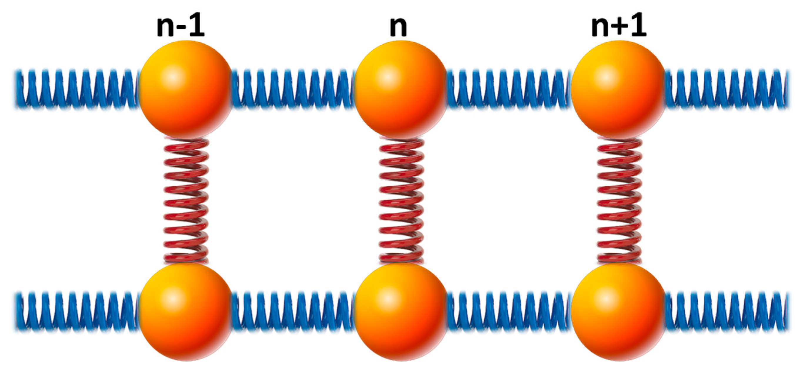
Let us consider a system composed of two coupled one-dimensional harmonic crystals as illustrated in Figure 1.

In absence of external forces, the equations describing the motion of atoms at location n in the two coupled 1-D harmonic crystals are given by:

$$m\frac{{\partial }^2{u}_n}{\partial t^2}=K_0\left(u_{n+1}-2u_n+u_{n-1}\right)+K_I\left(v_n-u_n\right)=0$$

(1a)

$$M\frac{{\partial }^2{v}_n}{\partial t^2}=K_0\left(v_{n+1}-2v_n+v_{n-1}\right)-K_I\left(v_n-u_n\right)=0$$

(1b)

here u and v represent the displacement in the upper and lower chains, respectively. These displacements can be visualized as being oriented along the chains. The side springs are illustrated for the sake of simplicity as vertical spring but physically they would couple masses between chains along the direction of the displacements.

In the long wavelength limit the discrete Lagrangian is expressed as a continuous second derivative of position. Taking $M=m$ for the sake of simplicity and mathematical tractability, the equations of motion (1a,b) can be rewritten as:

$$\left\{\left(\frac{{\partial }^2}{\partial t^2}-{\beta }^2\frac{{\partial }^2}{\partial x^2}\right)I+{\alpha }^{2}D\right\}U=0$$

(2)

where $I$ is the 2 × 2 identity matrix, $D=\left(\begin{array}{cc}1& -1\\ -1& 1\end{array}\right)$ and $U=\left(\begin{array}{c}u\\ v\end{array}\right)$ is the displacement vector. We also have defined ${\alpha }^2=\frac{K_I}{m}$ and ${\beta }^2=\frac{K_0}{m}$. Equation (2) takes a form similar to the Klein-Gordon equation. Using an approach paralleling that of Dirac, one can factor Equation (2) into the following form:

$$\left(\left[\mathrm{A}\frac{\partial }{\partial \mathrm{t}}+\mathsf{\beta }\text{B}\frac{\partial }{\partial \mathrm{x}}\right]-\mathrm{i}\frac{\mathsf{\alpha }}{\sqrt{2}}\mathrm{C}\right)\left(\left[\mathrm{A}\frac{\partial }{\partial \mathrm{t}}+\mathsf{\beta }\text{B}\frac{\partial }{\partial \mathrm{x}}\right]+\mathrm{i}\frac{\mathsf{\alpha }}{\sqrt{2}}\mathrm{C}\right)\mathsf{\Psi }=0$$

(3)

In Equation (3), we have introduced the 4 × 4 matrices: $A=\left(\begin{array}{cccc}0& 0& 1& 0\\ 0& 0& 0& 1\\ 1& 0& 0& 0\\ 0& 1& 0& 0\end{array}\right)$, $B=\left(\begin{array}{cccc}0& 0& 0& 1\\ 0& 0& 1& 0\\ 0& -1& 0& 0\\ -1& 0& 0& 0\end{array}\right)$, $C=\left(\begin{array}{cccc}1& -1& 0& 0\\ -1& 1& 0& 0\\ 0& 0& 1& -1\\ 0& 0& -1& 1\end{array}\right)$. The symbol i refers to $\sqrt{-1}$. The wave functions $\mathsf{\Psi }=\left(\begin{array}{c}{\psi }_1\\ {\psi }_2\\ {\psi }_3\\ {\psi }_4\end{array}\right)$ and $\overline{\mathsf{\Psi }}=\left(\begin{array}{c}{\overline{\psi }}_1\\ {\overline{\psi }}_2\\ {\overline{\psi }}_3\\ {\overline{\psi }}_4\end{array}\right)$ are 4 vector solutions of $\left(\left[A\frac{\partial }{\partial t}+\beta B\frac{\partial }{\partial x}\right]-i\frac{\alpha }{\sqrt{2}}C\right)\mathsf{\Psi }=0$ and $\left(\left[A\frac{\partial }{\partial t}+\beta B\frac{\partial }{\partial x}\right]+i\frac{\alpha }{\sqrt{2}}C\right)\overline{\mathsf{\Psi }}=0$, respectively. $\mathsf{\Psi }$ and $\overline{\mathsf{\Psi }}$ are non-self-dual solutions. These equations do not satisfy time reversal symmetry ($t\to -t)$, T-symmetry, nor parity symmetry ($x\to -x)$ separately. In the language of Quantum Field Theory, $\mathsf{\Psi }$ and $\overline{\mathsf{\Psi }}$ represent “particles” and “anti-particles”. Let us now seek solutions of $\left(\left[A\frac{\partial }{\partial t}+\beta B\frac{\partial }{\partial x}\right]-i\frac{\alpha }{\sqrt{2}}C\right)\mathsf{\Psi }=0$ in the plane wave form: ${\psi }_j=a_j{e}^{ikx}{e}^{i\omega t}$ with j = 1,2,3,4. This gives the eigen value problem:

$$\{\begin{array}{c}-\delta a_1+\delta a_2+\omega a_3+\beta k{a}_4=0\\ \delta a_1-\delta a_2+\beta k{a}_3+\omega a_4=0\\ \omega a_1-\beta k{a}_2-\delta a_3+\delta a_4=0\\ -\beta k{a}_1+\omega a_2+\delta a_3-\delta a_4=0\end{array}$$

(4)

where $\delta =\frac{\alpha }{\sqrt{2}}.$ We find two dispersion relations: $\omega =\pm \beta k$ and $\omega =\pm \sqrt{{\left(\beta k\right)}^2+2{\alpha }^2}$. The first set of dispersion relations corresponds to branches that start at the origin k = 0 and relates to symmetric eigen modes. The second set of branches represents antisymmetric modes with a cut off frequency at k = 0 of $\alpha \sqrt{2}$. Assuming that $a_1=a_2=a_F$ and that $a_3=a_4=a_B$, for the symmetric waves characterized by the first set of dispersion relations, then the Equation (4) reduce to $\left(\omega +\beta k\right)a_B=0$ and $\left(\omega -\beta k\right)a_F=0$ which are satisfied by plane waves of arbitrary amplitudes, $a_F$ and $a_B$, propagating in the forward (F) or backward (B) directions, respectively. This is the conventional character of Boson-like phonons. We now look for the eigen vectors that correspond to the second set of dispersion relations. Let us use the positive eigen value as an illustrative example:$\omega =+\sqrt{{\left(\beta k\right)}^2+2{\alpha }^2}$. One of the degenerate solutions of the system of four linear Equation (4) is:

$$\left(\begin{array}{c}{a}_1\\ a_2\\ a_3\\ a_4\end{array}\right)=a_0\left(\begin{array}{c}\sqrt{\omega -\beta k}\\ -\sqrt{\omega -\beta k}\\ \sqrt{\omega +\beta k}\\ -\sqrt{\omega +\beta k}\end{array}\right)$$

(5)

where$a_0$ is some arbitrary constant. Note that the negative signs reflect the antisymmetry of the displacement. Other solutions can be found by considering the complete set of plane wave solutions ${\psi }_j=a_j{e}^{\pm ikx}{e}^{\pm i\omega t}$ with j = 1,2,3,4 as well as the negative frequency eigen value. The key result is that the second dispersion curve in the band structure is associated with a wave function whose amplitude shows spinorial character (Equation (5)). In this case, the displacement of the two coupled harmonic chains are constrained and the direction of propagation of waves in the two-chain system are not independent of each other. For instance, at k = 0, the antisymmetric mode is represented by a standing wave which enforces a strict relation between the amplitude of a forward propagating wave and a backward propagating wave. This characteristic was shown [4,5] to be representative of Fermion-like behavior of phonons. 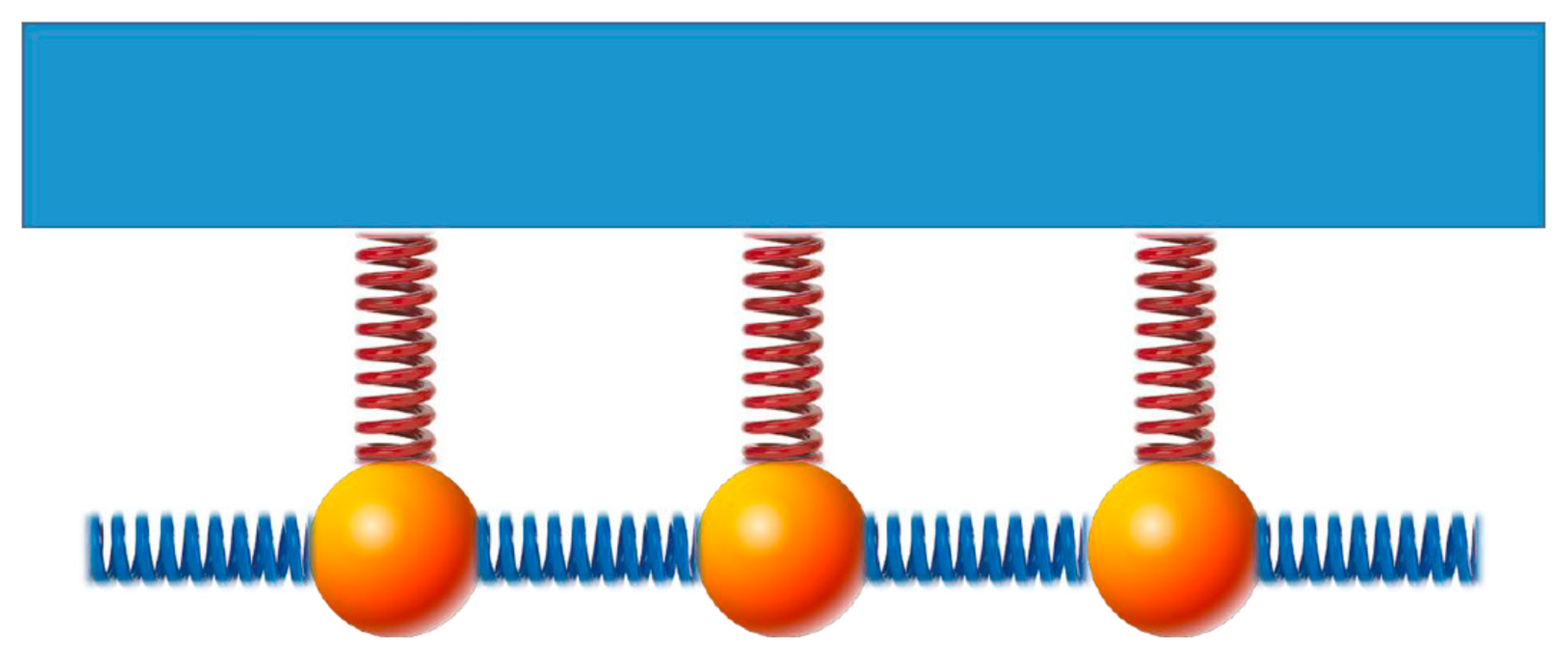As $k\to \infty$, $\omega \to +\beta k$, the first two terms in Equation (5) go to zero and only one direction of propagation (backward) is supported by the medium (third and fourth terms in Equation (5)). This example illustrates the difference in topology of elastic waves corresponding to the lower and upper bands in the band structure of the two-chain system. The constraint on the amplitude of waves in the upper band imparts a nonconventional spinorial topology to the eigen modes which does exists for modes in the lower band. The topology of the upper band can be best visualized by taking the limit $M\to \infty$. In that case, the system of Figure 1 becomes a single harmonic chain grounded to a substrate as shown in Figure 2.

In that limit, the displacement $v$ in Equation (1a,b) is negligible. Equation (2) becomes the Klein-Gordon equation: $\frac{{\partial }^{2}u}{\partial t^2}-{\beta }^2\frac{{\partial }^{2}u}{\partial x^2}+{\alpha }^{2}u=0$ with ${\alpha }^2=K_I/m$ and ${\beta }^2=K_0/m$. This equation describes only the displacement field, u. Equation (3) can be written as the set of Dirac-like equations:

$$\left[{\sigma }_x\frac{\partial }{\partial t}+i\beta {\sigma }_y\frac{\partial }{\partial x}-i\alpha I\right]\mathsf{\Psi }=0$$

(6a)

$$\left[{\sigma }_x\frac{\partial }{\partial t}+i\beta {\sigma }_y\frac{\partial }{\partial x}+i\alpha I\right]\overline{\mathsf{\Psi }}=0$$

(6b)

where ${\sigma }_x$ and ${\sigma }_y$ are the 2 × 2 Pauli matrices: $\left(\begin{array}{cc}0& 1\\ 1& 0\end{array}\right)$ and $\left(\begin{array}{cc}0& -i\\ i& 0\end{array}\right)$ and $I$ is the 2 × 2 identity matrix.

We now write our solutions in the form: ${\mathsf{\Psi }}_k=\mathsf{\Psi }\left(k,{\omega }_k\right)=c_0{\xi }_k\left(k,{\omega }_k\right)e^{(\pm )i{\omega }_{k}t}{e}^{(\pm )ikx}$ and ${\overline{\mathsf{\Psi }}}_k=\overline{\mathsf{\Psi }}\left(k,{\omega }_k\right)=c_0{\overline{\xi }}_k\left(k,{\omega }_k\right)e^{(\pm )i{\omega }_{k}t}{e}^{(\pm )ikx}$ where ${\xi }_k$ and ${\overline{\xi }}_k$ are two by one spinors. Inserting the various forms for these solutions in Equation (6a,b) lead to the same eigen values that we obtained before for the upper band of the two-chain system, namely by $\omega =\pm \sqrt{{\alpha }^2+{\beta }^2{k}^2}$. 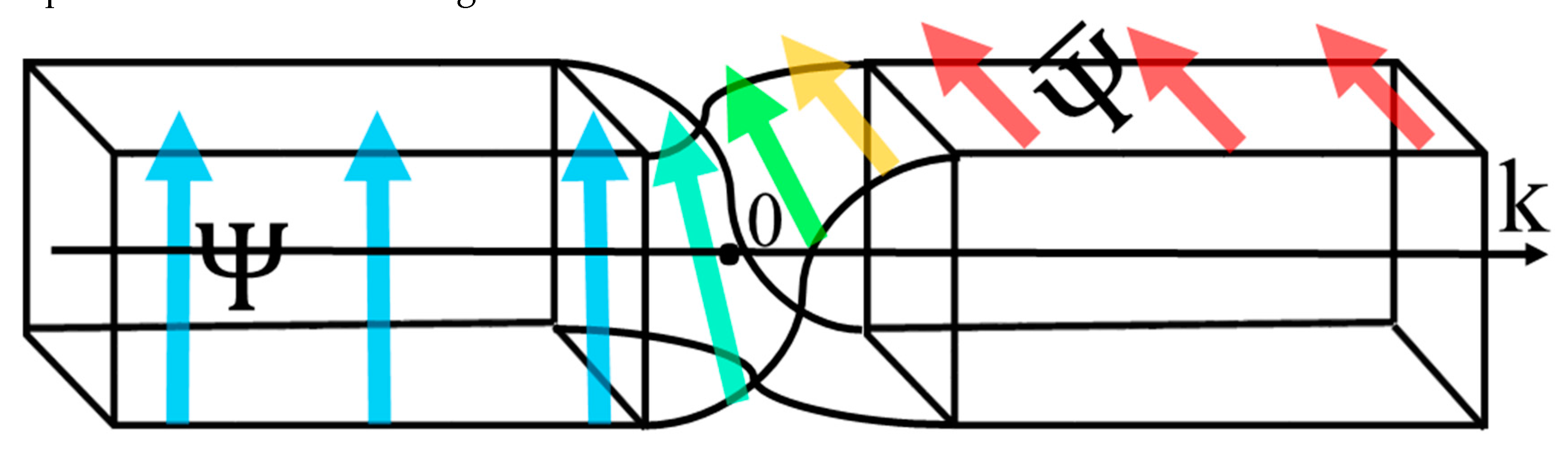Again, let us note that the band structure has two branches corresponding to positive frequencies and negative frequencies. Negative frequencies can be visualized as representing waves that propagate in a direction opposite to that of waves with positive frequency. The spinor part of the solutions for the different plane waves is summarized in the

Table 1. Two by one spinor solutions of Equation (6a,b) for the different plane wave forms.

	$e^{+ikx}{e}^{+i{\omega }_{k}t}$	$e^{-ikx}{e}^{+i{\omega }_{k}t}$	$e^{+ikx}{e}^{-i{\omega }_{k}t}$	$e^{-ikx}{e}^{-i{\omega }_{k}t}$
${\xi }_k$	$\left(\begin{array}{c}\sqrt{\omega +\beta k}\\ \sqrt{\omega -\beta k}\end{array}\right)$	$\left(\begin{array}{c}\sqrt{\omega -\beta k}\\ \sqrt{\omega +\beta k}\end{array}\right)$	$\left(\begin{array}{c}-\sqrt{\omega -\beta k}\\ \sqrt{\omega +\beta k}\end{array}\right)$	$\left(\begin{array}{c}-\sqrt{\omega +\beta k}\\ \sqrt{\omega -\beta k}\end{array}\right)$
${\overline{\xi }}_k$	$\left(\begin{array}{c}\sqrt{\omega -\beta k}\\ -\sqrt{\omega +\beta k}\end{array}\right)$	$\left(\begin{array}{c}\sqrt{\omega +\beta k}\\ -\sqrt{\omega -\beta k}\end{array}\right)$	$\left(\begin{array}{c}\sqrt{\omega +\beta k}\\ \sqrt{\omega -\beta k}\end{array}\right)$	$\left(\begin{array}{c}\sqrt{\omega -\beta k}\\ \sqrt{\omega +\beta k}\end{array}\right)$

below. Negative and positive k correspond to waves propagating in opposite direction.

Table 1 can be used to identify the symmetry properties of $\mathsf{\Psi }$ and $\overline{\mathsf{\Psi }}$ in the allowed space: $k, \omega$. We find the following transformation rules:

$$T_{\begin{array}{c}\omega \to \omega \\ k\to -k\end{array}}\left(\mathsf{\Psi }\left(\omega ,k\right)\right)=\mathsf{\Psi }\left(\omega ,k\right)$$

(7a)

$$T_{\begin{array}{c}\omega \to -\omega \\ k\to k\end{array}}\left(\mathsf{\Psi }\left(\omega ,k\right)\right)=i{\sigma }_x\overline{\mathsf{\Psi }}\left(-\omega ,k\right)$$

(7b)

which lead to the combined transformation:

$$T_{\begin{array}{c}\omega \to -\omega \\ k\to -k\end{array}}\left(\mathsf{\Psi }\left(\omega ,k\right)\right)=i{\sigma }_x\overline{\mathsf{\Psi }}\left(-\omega ,-k\right)$$

(8)

We have defined $T_{\begin{array}{c}\omega \to \omega \\ k\to -k\end{array}}$ and $T_{\begin{array}{c}\omega \to -\omega \\ k\to k\end{array}}$ as transformations that change the sign of the frequency and wave number, respectively. As one crosses the gap at the origin k = 0, the multiplicative factor “i” indicates that the wave function accumulated a phase of $\frac{\pi }{2}$. Also, the Pauli operator ${\sigma }_x$ enables the transition from the space of solutions $\mathsf{\Psi }$ to the space of $\overline{\mathsf{\Psi }}$. We also note the orthogonality condition $\overline{\mathsf{\Psi }}{\sigma }_x\mathsf{\Psi }=0.$ The topology of the spinorial wave functions that reflects their symmetry properties is illustrated in Figure 3.

We now shed more light on the properties of the spinorial solutions by treating $\alpha$ in Equation (6a,b) as a perturbation, $\epsilon$. When $\alpha =0$, Equation (6a) reduces to the two independent equations:

$$\left(\frac{\partial }{\partial t}-\beta \frac{\partial }{\partial x}\right){\phi }_1^{\left(0\right)}=0$$

(9a)

$$\left(\frac{\partial }{\partial t}-\beta \frac{\partial }{\partial x}\right){\phi }_1^{\left(0\right)}=0$$

(9b)

whose solutions correspond to plane waves propagating in the forward direction,${\phi }_1^{\left(0\right)}$, with dispersion relation ${\omega }^{+}=\beta k$ and the backward direction, ${\phi }_2^{\left(0\right)}$ with dispersion relation ${\omega }^{-}=-\beta k$. We rewrite Equation (9) in the form:

$$\left(\frac{\partial }{\partial t}-\beta \frac{\partial }{\partial x}\right){\phi }_1=i\epsilon {\phi }_2^{\left(0\right)}=i\epsilon e^{ikx}{e}^{{\omega }^{-}t}$$

(10a)

$$\left(\frac{\partial }{\partial t}+\beta \frac{\partial }{\partial x}\right){\phi }_2=i\epsilon {\phi }_1^{\left(0\right)}=i\epsilon e^{ikx}{e}^{{\omega }^{+}t}$$

(10b)

Seeking the particular solutions to first-order, ${\phi }_1^{\left(1\right)}$ and ${\phi }_2^{\left(1\right)}$, which follow in frequency the driving terms on the right-side side of Equation (10a,b), we find their respective amplitude to be:

$$a_1=\frac{\epsilon }{{\omega }^{-}-\beta k}=\frac{\epsilon }{{\omega }^{-}-{\omega }^{+}}$$

(11a)

$$a_2=\frac{\epsilon }{{\omega }^{+}+\beta k}=\frac{\epsilon }{{\omega }^{+}-{\omega }^{-}}=-a_1$$

(11b)

Since ${\omega }^{+}={\omega }^{-}$ at k = 0 only, the amplitude of the first-order perturbed forward wave, $a_1$ changes sign as k varies from $-\infty$ to $+\infty$. A similar but opposite change of sign occurs for the backward perturbed amplitude. These changes of sign are therefore associated with changes in phase of $\pi$ and −$\pi$ for the forward and backward waves as one crosses the origin k = 0. These phase changes (sign changes) are characteristic of that occurring at a resonance. The gap that would occur at k = 0 in the band structure of the harmonic chain grounded to a substrate via side springs, should we push the perturbation theory to higher orders, may therefore be visualized as resulting from a resonance of the forward waves driven by the backward propagating waves and vice versa. However, since to first-order the amplitudes given by Equation (11a,b) diverge at the only point of intersection between the dispersion relations of the forward and backward waves, we have to use analytic continuation to expand them into the complex plane:

$$a_1^{+}=\frac{\epsilon }{{\omega }^{-}-\beta k-i\eta }=\frac{\epsilon }{-2\beta k-i\eta }$$

(12a)

$$a_2^{+}=\frac{\epsilon }{{\omega }^{+}+\beta k+i\eta }=\frac{\epsilon }{+2\beta k+i\eta }$$

(12b)

where $\eta \to 0$ continues the eigen values ${\omega }^{-}$ and ${\omega }^{+}$ into the complex plane.

By simple inspection, we can see that at the origin, k = 0, both amplitudes are pure imaginary quantities and therefore exhibit a phase of $\pm \frac{\pi }{2}$. This is expected as Equation (12a,b) are representative of the amplitude of a driven damped harmonic oscillator which also shows a phase of $\frac{\pi }{2}$ with respect to the driving frequency at resonance. It is instructive to calculate the Berry connection [31] for these perturbed amplitudes. The Berry connection determines the phase change of a wave as some parameter takes the wave function along a continuous path on the manifold that supports it. Since the Berry phase applies to continuous paths, we cannot use that concept to determine the phase change across the gap of our system, i.e., between the positive and negative frequency branches of the band structure. Therefore, we resort to calculating the Berry connection for the first-order perturbed solution which still remains continuous but may capture the interaction between directions of propagation. Our intention is to characterize the topology of the spinorial part of the wave function Equation (12a,b), by calculating the change in phase of the waves as one crosses k = 0. It is important first to normalize the spinor: $\xi =\left(\begin{array}{c}{a}_1^{+}\\ a_2^{+}\end{array}\right)$. This normalized spinor takes the form: $\tilde{\xi }=\left(\begin{array}{c}{\tilde{a}}_1^{+}\\ {\tilde{a}}_2^{+}\end{array}\right)=\frac{\sqrt{4{\beta }^2{k}^2+{\eta }^2}}{\sqrt{2}}\left(\begin{array}{c}\frac{1}{-2\beta k-i\eta }\\ \frac{1}{+2\beta k+i\eta }\end{array}\right)$. The Berry connection is given by $A\left(k\right)=-i{\tilde{\xi }}^{*}\frac{\partial \tilde{\xi }}{\partial k}=-i{\tilde{a}}_1^{+}{}^{*}\frac{\partial {\tilde{a}}_1^{+}}{\partial k}-i{\tilde{a}}_2^{+}{}^{*}\frac{\partial {\tilde{a}}_2^{+}}{\partial k}$. After several analytical and algebraic manipulations, we obtain:

$$A\left(k\right)=\beta \frac{\eta }{4{\beta }^2{k}^2+{\eta }^2}+\beta \frac{\eta }{4{\beta }^2{k}^2+{\eta }^2}$$

(13)

In Equation (13), the contribution to the Berry connection of ${\tilde{a}}_1^{+}$ and ${\tilde{a}}_2^{+}$ are identical. Using the identities: $\underset{\eta \to 0}{\lim }\frac{\eta }{x^2+{\eta }^2}=\pi \delta \left(x\right)$ and $\delta \left(ax\right)=\frac{1}{a}\delta \left(x\right)$, leads to

$$A\left(k\right)=\frac{\pi }{2}\delta \left(k\right)+\frac{\pi }{2}\delta \left(k\right)$$

(14)

The contribution of each direction of propagation to the spinorial part of the wave function accumulates a $\frac{\pi }{2}$ phase shift as one crosses the origin k = 0.

3. Extrinsic Phononic Structure

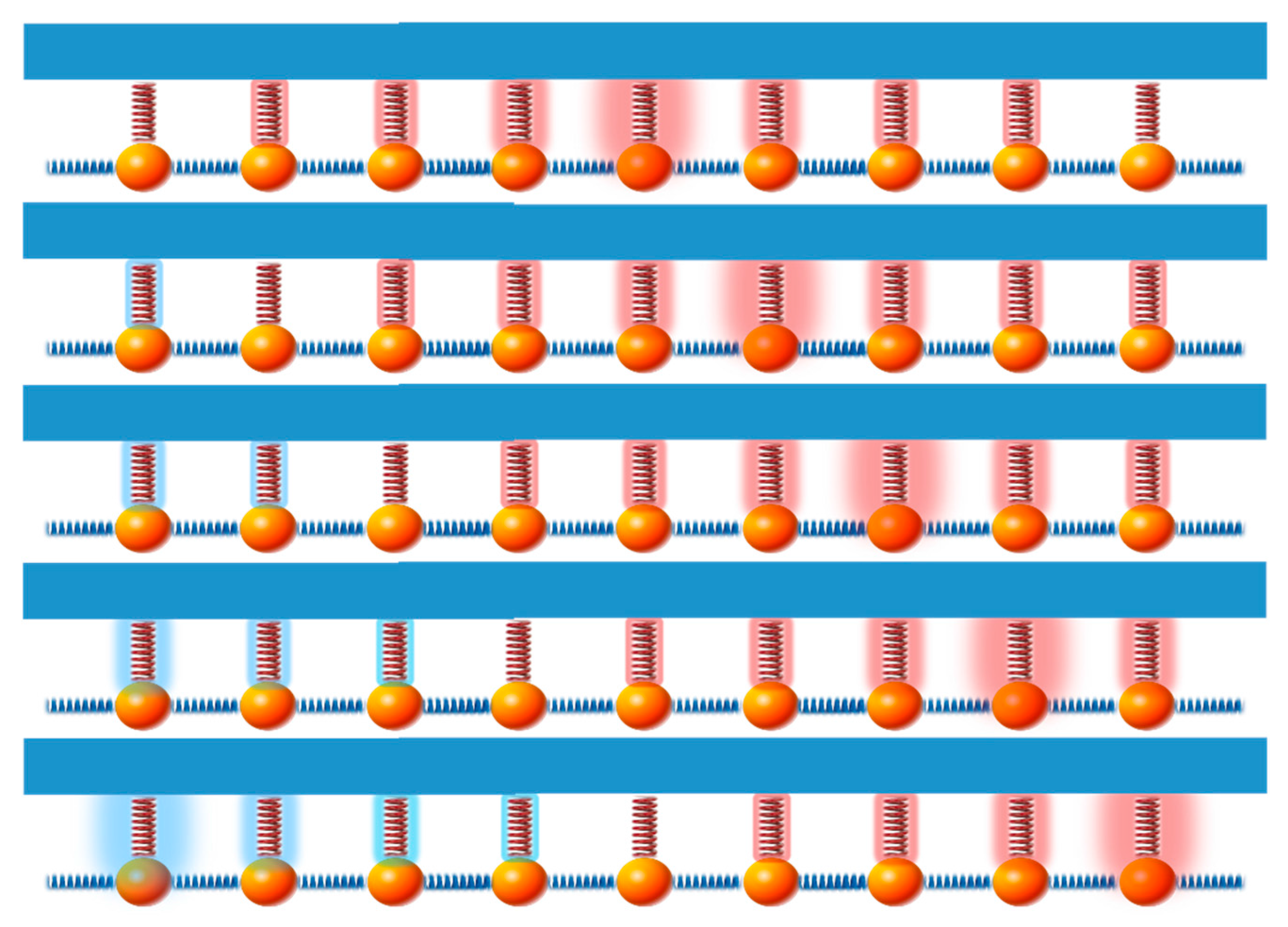
In the previous section, we revealed the spinorial character of the elastic wave function in the two-chain system and one chain coupled to the ground. The purpose of this section is to investigate the behavior of field $\mathsf{\Psi }$ when the parameter $\alpha$ (spring stiffness, K_I) is subjected to a spatio-temporal modulation, i.e., $\alpha ={\alpha }_0+{\alpha }_{1}2\sin \left(Kx+\mathsf{\Omega }t\right)$ where ${\alpha }_0$ and ${\alpha }_1$ are constants (see Figure 4). Here, $K=\frac{2\pi }{L}$ where $L$ is the period of the modulation. $\mathsf{\Omega }$ is the frequency modulation and its sign determines the direction of propagation of the modulation.

The question arises as to the effect of such a modulation on the state of the fermion-like phonons. The periodicity of the modulated one-dimensional medium suggests that we should be seeking solutions of Equation (1) in the form of Bloch waves: $\mathsf{\Psi }\left(x,t\right)={\sum }_k{\sum }_g\psi \left(k,g,t\right)e^{i\left(k+g\right)x}$ where $x\in \left[0,L\right]$. The wave number $k$ is limited to the first Brillouin zone: $\left[\frac{-\pi }{L},\frac{\pi }{L}\right]$ and $g=\frac{2\pi }{L}l$ with l being an integer. Choosing Equation (6a), we obtain the modulated Dirac-like equation in the Fourier domain:

$$\begin{array}{c}\left[{\sigma }_x\frac{\partial }{\partial t}+i\beta {\sigma }_y\left(i{k}^{*}\right)-i{\alpha }_{0}I\right]\psi \left(k^{*},t\right)\\ -{\alpha }_{1}I\left[\psi \left(k^{*}+K,t\right)e^{i\mathsf{\Omega }t}-\psi \left(k^{*}-K,t\right)e^{-i\mathsf{\Omega }t}\right]=0\end{array}$$

(15)

where $k^{*}=k+g$.

Consistent with Quantum Field Theory (QFT) approaches, we solve Equation (15) using perturbation theory and in particular multiple time scale perturbation theory [32] up to second-order. Nowadays, the multiple-time-scales perturbation theory (MTSPT) for differential equations is a very popular method to approximate solutions of weakly nonlinear differential equations. Several implementations of this method were proposed in various fields of mathematics, mechanics and physics [33,34,35,36,37,38]. Moreover, Khoo et al. [39] have shown that the MTSPT is a reliable theoretical tool for studying the lattice dynamics of an anharmonic crystal. More recently, Swinteck et al. [40] applied successfully the MTSPT, as described in Reference [19], for solving propagation equations in a quadratically nonlinear monoatomic chain of infinite extent. Consequently, we used the MTSPT for solving Equation (15).

The parameter ${\alpha }_1$ is treated as a perturbation $\epsilon$. The wave function is written as a second-order power series in $\epsilon$, namely:

$$\psi \left(k^{*},{\tau }_0,{\tau }_1,{\tau }_2\right)={\psi }^{\left(0\right)}\left(k^{*},{\tau }_0,{\tau }_1,{\tau }_2\right)+\epsilon {\psi }^{\left(1\right)}\left(k^{*},{\tau }_0,{\tau }_1,{\tau }_2\right)+{\epsilon }^2{\psi }^{\left(2\right)}\left(k^{*},{\tau }_0,{\tau }_1,{\tau }_2\right)$$

here ${\psi }^{\left(j\right)}$ with $j=0,1,2$ are wave functions expressed to zeroth, first and second-order. We have also replaced the single time variable, $t$, by three variables representing different time scales: ${\tau }_0=t$, ${\tau }_1=\epsilon t$, and ${\tau }_2={\epsilon }^{2}t={\epsilon }^2{\tau }_0$. We can subsequently decompose Equation (15) into equations to zeroth, first and second-order in $\epsilon$. The zeroth-order equation consists of the Dirac-like equation in absence of modulation:

$$\left[{\sigma }_x\frac{\partial }{\partial {\tau }_0}+i\beta {\sigma }_y\left(i{k}^{*}\right)-i{\alpha }_{0}I\right]{\psi }^{\left(0\right)}\left(k^{*},{\tau }_0,{\tau }_1,{\tau }_2\right)=0$$

(16)

As seen in Section 2, its solutions take the form ${\psi }^{\left(0\right)}\left(k^{*},{\tau }_0,{\tau }_1,{\tau }_2\right)=a^{\left(0\right)}\left(k^{*},{\tau }_1,{\tau }_2\right)e^{i{\omega }_0{\tau }_0}$ with $a^{\left(0\right)}\left(k^{*},{\tau }_1,{\tau }_2\right)=\left(\begin{array}{c}{a}_1^{\left(0\right)}\\ a_2^{\left(0\right)}\end{array}\right)=a_0\left(\begin{array}{c}\sqrt{{\omega }_0+\beta k^{*}}\\ \sqrt{{\omega }_0-\beta k^{*}}\end{array}\right)$. $e^{i{\omega }_0{\tau }_0}$ and $a^{\left(0\right)}$ represent the orbital and the spinorial parts of the solution, respectively. We have the usual eigen values: ${\omega }_0^2={\alpha }^2+{\beta }^2{\left(k^{*}\right)}^2$. Inserting the zeroth-order solution into Equation (15) expressed to first-order leads to

$$\begin{array}{c}\left[{\sigma }_x\frac{\partial }{\partial {\tau }_0}+i\beta {\sigma }_y\left(i{k}^{*}\right)-i{\alpha }_{0}I\right]{\psi }^{\left(1\right)}\left(k^{*},{\tau }_0,{\tau }_1,{\tau }_2\right)=-{\sigma }_x\frac{\partial }{\partial {\tau }_1}{\psi }^{\left(0\right)}\left(k^{*},{\tau }_0,{\tau }_1,{\tau }_2\right)\\ I\left[{\psi }^{\left(0\right)}\left(k^{*}+K,{\tau }_0,{\tau }_1,{\tau }_2\right)e^{i\mathsf{\Omega }{\tau }_0}-{\psi }^{\left(0\right)}\left(k^{*}-K,{\tau }_0,{\tau }_1,{\tau }_2\right)e^{-i\mathsf{\Omega }{\tau }_0}\right]\end{array}$$

(17)

The solutions of the first-order Dirac equation are the sum of solutions of the homogeneous equation and particular solutions. The homogenous solution is isomorphic to the zeroth-order solution, it will be corrected in a way similar to the zeroth-order solution as one accounts for higher and higher terms in the perturbation series. Under these conditions and to ensure that there are no secular terms (i.e., terms that grow with time and that are incompatible with the assumption that ${\psi }^{\left(1\right)}$ must be a correction to ${\psi }^{\left(0\right)}$ in the particular solution of Equation (17), the pre-factors of terms like $e^{i{\omega }_0{\tau }_0}$ are forced to be zero [39]. Subsequently, the derivative of the amplitudes $a^{\left(0\right)}\left(k^{*}, {\tau }_1,{\tau }_2\right)$ with respect to ${\tau }_1$ must vanish and these amplitudes only depend on ${\tau }_2$. The right-hand side of Equation (17) reduces to the second term only. The particular solution of that simplified equation contains frequency shifted terms given by:

$${\psi }_{1,P}^{\left(1\right)}=b_1{e}^{i\left({\omega }_0+\mathsf{\Omega }\right){\tau }_0}+b_1^{\prime }{e}^{i\left({\omega }_0-\mathsf{\Omega }\right){\tau }_0}$$

$${\psi }_{2,P}^{\left(1\right)}=b_2{e}^{i\left({\omega }_0+\mathsf{\Omega }\right){\tau }_0}+b_2^{\prime }{e}^{i\left({\omega }_0-\mathsf{\Omega }\right){\tau }_0}$$

The coefficients $b_1,b_1^{\prime },b_2,b_2^{\prime }$ are resonant terms:

$$b_1\left(k^{*}\right)=\frac{i}{{\alpha }_0}{a}_1^{\left(0\right)}\left(k^{*}+K\right)+\frac{1}{{\alpha }_0}{b}_2\left(k^{*}\right)\left[\left({\omega }_0+\mathsf{\Omega }\right)+\beta k^{*}\right]$$

$$b_1^{\prime }\left(k^{*}\right)=\frac{-i}{{\alpha }_0}{a}_1^{\left(0\right)}\left(k^{*}-K\right)+\frac{1}{{\alpha }_0}{b}_2^{\prime }\left(k^{*}\right)\left[\left({\omega }_0-\mathsf{\Omega }\right)+\beta k^{*}\right]$$

$$b_2\left(k^{*}\right)=-i\frac{\left\{a_1^{\left(0\right)}\left(k^{*}+K\right)\left[\left({\omega }_0+\mathsf{\Omega }\right)-\beta k^{*}\right]+{\alpha }_0{a}_2^{\left(0\right)}\left(k^{*}+K\right)\right\}}{{\left({\omega }_0+\mathsf{\Omega }\right)}^2-{\left(\beta k^{*}\right)}^2-{\alpha }_0^2}$$

$$b_2^{\prime }\left(k^{*}\right)=+i\frac{\left\{a_1^{\left(0\right)}\left(k^{*}-K\right)\left[\left({\omega }_0-\mathsf{\Omega }\right)-\beta k^{*}\right]+{\alpha }_0{a}_2^{\left(0\right)}\left(k^{*}-K\right)\right\}}{{\left({\omega }_0-\mathsf{\Omega }\right)}^2-{\left(\beta k^{*}\right)}^2-{\alpha }_0^2}$$

In the preceding relations, we have defined: ${\omega }_0+\mathsf{\Omega }={\omega }_0\left(k^{*}+K\right)+\mathsf{\Omega }$ and ${\omega }_0-\mathsf{\Omega }={\omega }_0\left(k^{*}-K\right)+\mathsf{\Omega }$. We have also omitted the time dependencies for the sake of compactness.

To second order, the Dirac-like equation is written as:

$$\begin{array}{c}\left[{\sigma }_x\frac{\partial }{\partial {\tau }_0}+i\beta {\sigma }_y\left(i{k}^{*}\right)-i{\alpha }_{0}I\right]{\psi }^{\left(2\right)}\left(k^{*},{\tau }_0,{\tau }_2\right)=\\ -{\sigma }_x\frac{\partial {\psi }^{\left(0\right)}\left(k^{*},{\tau }_0,{\tau }_2\right)}{\partial {\tau }_2}+I\left[{\psi }^{\left(1\right)}\left(k^{*}+K,{\tau }_0,{\tau }_2\right)e^{i\mathsf{\Omega }{\tau }_0}-{\psi }^{\left(1\right)}\left(k^{*}-K,{\tau }_0,{\tau }_2\right)e^{-i\mathsf{\Omega }{\tau }_0}\right]\end{array}$$

(18)

$\left[{\sigma }_x\frac{\partial }{\partial {\tau }_0}+i\beta {\sigma }_y\left(i{k}^{*}\right)-i{\alpha }_{0}I\right]{\psi }^{\left(2\right)}\left(k^{*},{\tau }_0,{\tau }_2\right)=$The derivative $\frac{\partial {\psi }^{\left(0\right)}\left(k^{*},{\tau }_0,{\tau }_2\right)}{\partial {\tau }_2}$ leads to secular terms. The homogeneous part of the first-order solution does not contribute secular terms but the particular solution does. Combining all secular terms and setting them to zero lead to the conditions:

$$\frac{\partial a_1^{\left(0\right)}\left(k^{*}\right)}{\partial {\tau }_2}=i{a}_1^{\left(0\right)}\left(k^{*}\right)G^{\prime }+i{a}_2^{\left(0\right)}\left(k^{*}\right)F$$

(19a)

$$\frac{\partial a_2^{\left(0\right)}\left(k^{*}\right)}{\partial {\tau }_2}=i{a}_1^{\left(0\right)}\left(k^{*}\right)F+i{a}_2^{\left(0\right)}\left(k^{*}\right)G$$

(19b)

where we have defined:

$$F={\alpha }_0\left\{\frac{1}{{\left({\omega }_0\left(k^{*}\right)-\mathsf{\Omega }\right)}^2-{\omega }_0^2\left(k^{*}+K\right)}+\frac{1}{{\left({\omega }_0\left(k^{*}\right)+\mathsf{\Omega }\right)}^2-{\omega }_0^2\left(k^{*}-K\right)}\right\}$$

$$G=\left\{\frac{\left({\omega }_0\left(k^{*}\right)-\mathsf{\Omega }\right)+\beta \left(k^{*}+K\right)}{{\left({\omega }_0\left(k^{*}\right)-\mathsf{\Omega }\right)}^2-{\omega }_0^2\left(k^{*}+K\right)}+\frac{\left({\omega }_0\left(k^{*}\right)+\mathsf{\Omega }\right)+\beta \left(k^{*}-K\right)}{{\left({\omega }_0\left(k^{*}\right)+\mathsf{\Omega }\right)}^2-{\omega }_0^2\left(k^{*}-K\right)}\right\}$$

$$G\prime =\left\{\frac{\left({\omega }_0\left(k^{*}\right)-\mathsf{\Omega }\right)-\beta \left(k^{*}+K\right)}{{\left({\omega }_0\left(k^{*}\right)-\mathsf{\Omega }\right)}^2-{\omega }_0^2\left(k^{*}+K\right)}+\frac{\left({\omega }_0\left(k^{*}\right)+\mathsf{\Omega }\right)-\beta \left(k^{*}-K\right)}{{\left({\omega }_0\left(k^{*}\right)+\mathsf{\Omega }\right)}^2-{\omega }_0^2\left(k^{*}-K\right)}\right\}$$

We note the asymmetry of these quantities. The terms G, G’ and F diverge within the Brillouin zone of the modulated systems when the condition ${\left({\omega }_0\left(k^{*}\right)+\mathsf{\Omega }\right)}^2-{\omega }_0^2\left(k^{*}-K\right)\to 0$ is satisfied but not when ${\left({\omega }_0\left(k^{*}\right)-\mathsf{\Omega }\right)}^2-{\omega }_0^2\left(k^{*}+K\right)\to 0$. This asymmetry reflects a breaking of symmetry in wave number space due to the directionality of the modulation.

Equation (19a,b) impose second-order corrections onto the zeroth-order solution. We multiply the relations (18a,b) by ${\epsilon }^2{e}^{i{\omega }_0{\tau }_0}$ to obtain them in terms of ${\psi }^{\left(0\right)}$ and subsequently recombine them with the zeroth-order Equation (3). This procedure reconstructs the perturbative series of Equation (15) in terms of ${\psi }^{\left(0\right)}$ only:

$$\left[{\sigma }_x\left(\frac{\partial }{\partial t}-i{\varnothing }_{k^{*}}\right)+i\beta {\sigma }_y\left(i{k}^{*}-i{A}_{k^{*}}\right)-i\left({\alpha }_0+m_{k^{*}}\right)I\right]{\psi }^{\left(0\right)}\left(k^{*},t\right)=0$$

(20)

with $\left(\begin{array}{c}{\varnothing }_{k^{*}}\\ A_{k^{*}}\end{array}\right)=\left(\begin{array}{c}\frac{{\epsilon }^2}{2}\left(G+G^{\prime }\right)\\ \frac{{\epsilon }^2}{2\beta }\left(G-G^{\prime }\right)\end{array}\right)$ and $m_{k^{*}}={\epsilon }^{2}F$. To obtain Equation (20), we have also used: $\frac{\partial }{\partial t}=\frac{\partial }{\partial {\tau }_0}+{\epsilon }^2\frac{\partial }{\partial {\tau }_2}$. Equation (20) shows that Equation (15) describing the dynamics of elastic waves in a harmonic chain grounded to a substrate via side springs, whose stiffness is modulated in space and time, is to second-order isomorphic to Dirac equation in Fourier domain for a charged quasiparticle including an electromagnetic field. The quantity ${\varnothing }_{k^{*}}$ plays the role of the electrostatic potential and $A_{k^{*}}$ the role of a scalar form of the vector potential. The parentheses $\left(\frac{\partial }{\partial t}-i{\varnothing }_{k^{*}}\right)$ and $\left(i{k}^{*}-i{A}_{k^{*}}\right)$ are the Fourier transforms of the usual minimal substitution rule. ${\alpha }_0+m_{k^{*}}$ is the dressed mass of the quasiparticle. The mechanical system provides a mechanism for exchange of energy between the main chain modes and the side springs. The side springs lead to the formation of a fermion-like quasiparticle while their modulation provides a field through which quasiparticles interact. The strength and nature of the interaction is controllable through the independent modulation parameters, ${\alpha }_1$ ,$\mathsf{\Omega }$ and K.

The mechanical system allows for the exploration of a large parameter space of scalar QFT as the functions ${\varnothing }_{k^{*}}$ and $A_{k^{*}}$ can be varied by manipulating the spatio-temporal modulation of the side spring stiffness. We imagine, therefore, that this classical phononic system can be employed to examine the behavior of scalar QFT from weak to strong coupling regimes, as well as, at all intermediate couplings. Further, the capacity to separate the ratio of the effective potentials opens avenues for the experimental realization of scalar fields whose behavior could previously only have been theorized.

We now seek solutions of Equation (20). These are solutions of Equation (18) with spinorial part $a^{\left(0\right)}\left(k^{*}, {\tau }_2\right)$ satisfying the second-order conditions given by Equation (19a,b). These conditions can be reformulated as $\frac{\partial \tilde{a}}{\partial {\tau }_2}=iM\tilde{a}$ where the vector $\tilde{a}=\left(\begin{array}{c}{a}_1^{\left(0\right)}\\ a_2^{\left(0\right)}\end{array}\right)$ and the matrix $M=\left(\begin{array}{cc}G\prime & F\\ F& G\end{array}\right)$. Solutions of this 2 × 2 system of first-order linear equations are easily obtained as: $\tilde{a}=C\tilde{e}{e}^{i\lambda {\tau }_2}+C\prime {\tilde{e}}^{\prime }{e}^{i{\lambda }^{\prime }{\tau }_2}$ where ${\lambda }^{\prime },$ $\tilde{e}$, and${\tilde{e}}^{\prime }$ are the eigen values and eigen vectors of the matrix $M$. The coefficients C and C’ are determined by the boundary condition: $\underset{\epsilon \to 0}{\lim }\tilde{a}=a_0\left(\begin{array}{c}\sqrt{{\omega }_0+\beta k^{*}}\\ \sqrt{{\omega }_0-\beta k^{*}}\end{array}\right)$. We find the eigen values $\lambda =\frac{G+G\prime }{2}+\sqrt{{\left(\frac{G-G\prime }{2}\right)}^2+F^2}$ and $\lambda \prime =\frac{G+G\prime }{2}-\sqrt{{\left(\frac{G-G\prime }{2}\right)}^2+F^2}$. The respective eigen vectors are $\tilde{e}=a_0\sqrt{{\omega }_0\left(k^{*}\right)+\beta k^{*}}F\left(\begin{array}{c}1\\ \frac{G-G\prime }{2F}+\sqrt{{\left(\frac{G-G\prime }{2F}\right)}^2+1}\end{array}\right)$ and ${\tilde{e}}^{\prime }=a_0\sqrt{{\omega }_0\left(k^{*}\right)+\beta k^{*}}F\left(\begin{array}{c}1\\ \frac{G-G\prime }{2F}-\sqrt{{\left(\frac{G-G\prime }{2F}\right)}^2+1}\end{array}\right)$. The coefficients are given by $C=\frac{1}{F}\frac{1}{2\sqrt{{\left(\frac{G-G\prime }{2F}\right)}^2+1}}\left\{\frac{\sqrt{{\omega }_0\left(k^{*}\right)-\beta k^{*}}}{\sqrt{{\omega }_0\left(k^{*}\right)+\beta k^{*}}}-\frac{G-G\prime }{2F}+\sqrt{{\left(\frac{G-G\prime }{2F}\right)}^2+1}\right\}$ and $C^{\prime }=\frac{1}{F}\frac{1}{2\sqrt{{\left(\frac{G-G^{\prime }}{2F}\right)}^2+1}}\left\{-\frac{\sqrt{{\omega }_0\left(k^{*}\right)-\beta k^{*}}}{\sqrt{{\omega }_0\left(k^{*}\right)+\beta k^{*}}}+\frac{G-G^{\prime }}{2F}+\sqrt{{\left(\frac{G-G^{\prime }}{2F}\right)}^2+1}\right\}$. We note that although the quantities G, G’ and F may diverge the ratio $\frac{G-G\prime }{2F}$ remains finite. The directed spatio-temporal modulation impacts both the orbital part and the spinor part of the zeroth-order modes. The orbital part of the wave function is frequency shifted to ${\omega }_0+{\epsilon }^2\lambda$ and ${\omega }_0+{\epsilon }^2{\lambda }^{\prime }$. The quantities ${\epsilon }^2\lambda t$ and ${\epsilon }^2{\lambda }^{\prime }t$ represent phase shifts analogous to those associated with the Aharonov-Bohm effect [41] resulting from electrostatic and vector potentials ${\varnothing }_{k^{*}}$ and $A_{k^{*}}$. Near the resonant condition: ${\left({\omega }_0\left(k^{*}\right)+\mathsf{\Omega }\right)}^2-{\omega }_0^2\left(k^{*}-K\right)\to 0$, it is the eigen value $\lambda \to \frac{1}{\left({\omega }_0\left(k^{*}\right)+\mathsf{\Omega }\right)-{\omega }_0\left(k^{*}-K\right)}$ which diverges. This divergence is indicative of the formation of a gap in the dispersion relation [31]. The eigen value $\lambda \prime \to \frac{1}{\left({\omega }_0\left(k^{*}\right)+\mathsf{\Omega }\right)+{\omega }_0\left(k^{*}-K\right)}~\frac{1}{2\left({\omega }_0\left(k^{*}\right)+\mathsf{\Omega }\right)}$ does not diverge. Since the frequency shift, ${\epsilon }^2{\lambda }^{\prime }$, is expected to be small compared to ${\omega }_0\left(k^{*}\right)$, the orbital term $e^{i\lambda {\tau }_2}\to 1$. Considering that the lowest frequency ${\omega }_0$ is ${\alpha }_0$, this condition would occur for all k*. Therefore, the term $e^{i({\omega }_0+{\epsilon }^2{\lambda }^{\prime }){\tau }_0}~e^{i{\omega }_0{\tau }_0}$ will essentially contribute to the band structure in a perturbative way similar to that of the uncorrected zeroth-order solution or homogeneous parts of the first or second-order equations. The spinorial part of the zeroth-order solution is also modified through the coupling between the orbital and “spin” part of the wave function as seen in the expressions for $\tilde{e}$and ${\tilde{e}}^{\prime }$. This coupling suggests an approach for the manipulation of the “spin” part of the elastic wave function by exciting the medium using a spatio-temporal modulation. Again, these alterations can be achieved by manipulating independently the magnitude of the modulation, ${\alpha }_1$ as well as the spatio-temporal characteristics $\mathsf{\Omega }$ and K.

The perturbative approach used here is showing the capacity of a spatio-temporal modulation to control the “spin-orbit” characteristics of elastic modes in a manner analogous to electromagnetic waves enabling the manipulation of the spin state of electrons [42]. However, the pertubative method is not able to give a complete picture of the effect of the modulation on the entire band structure of the elastic modes. For this, the vibrational properties of the mechanical system are also investigated numerically beyond perturbation theory. We calculate the phonon band structure of the modulated elastic Klein-Gordon equation since its eigen values are identical to those of the modulated Dirac-like equation. We use a one-dimensional chain that contains N = 2400 masses, m = 4.361 × 10⁻⁹ kg, with Born-Von Karman boundary conditions. The masses are equally spaced by h = 0.1 mm. The parameters $K_0$ = 0.018363 kg·m²·s⁻² and $K_I$ = 2295 kg·s⁻². The spatial modulation has a period L = 100 h and an angular frequency $\mathsf{\Omega }$ = 1.934 × 10⁵ rad/s. We have also chosen the magnitude of the modulation: ${\alpha }_1=\frac{1}{10}{\alpha }_0$. The dynamics of the modulated system is amenable to the method of molecular dynamics (MD). The integration time step is dt = 1.624 × 10^-9 s. The dynamical trajectories generated by the MD simulation are analyzed within the framework of the Spectral Energy Density (SED) method [43] for generating the band structure. 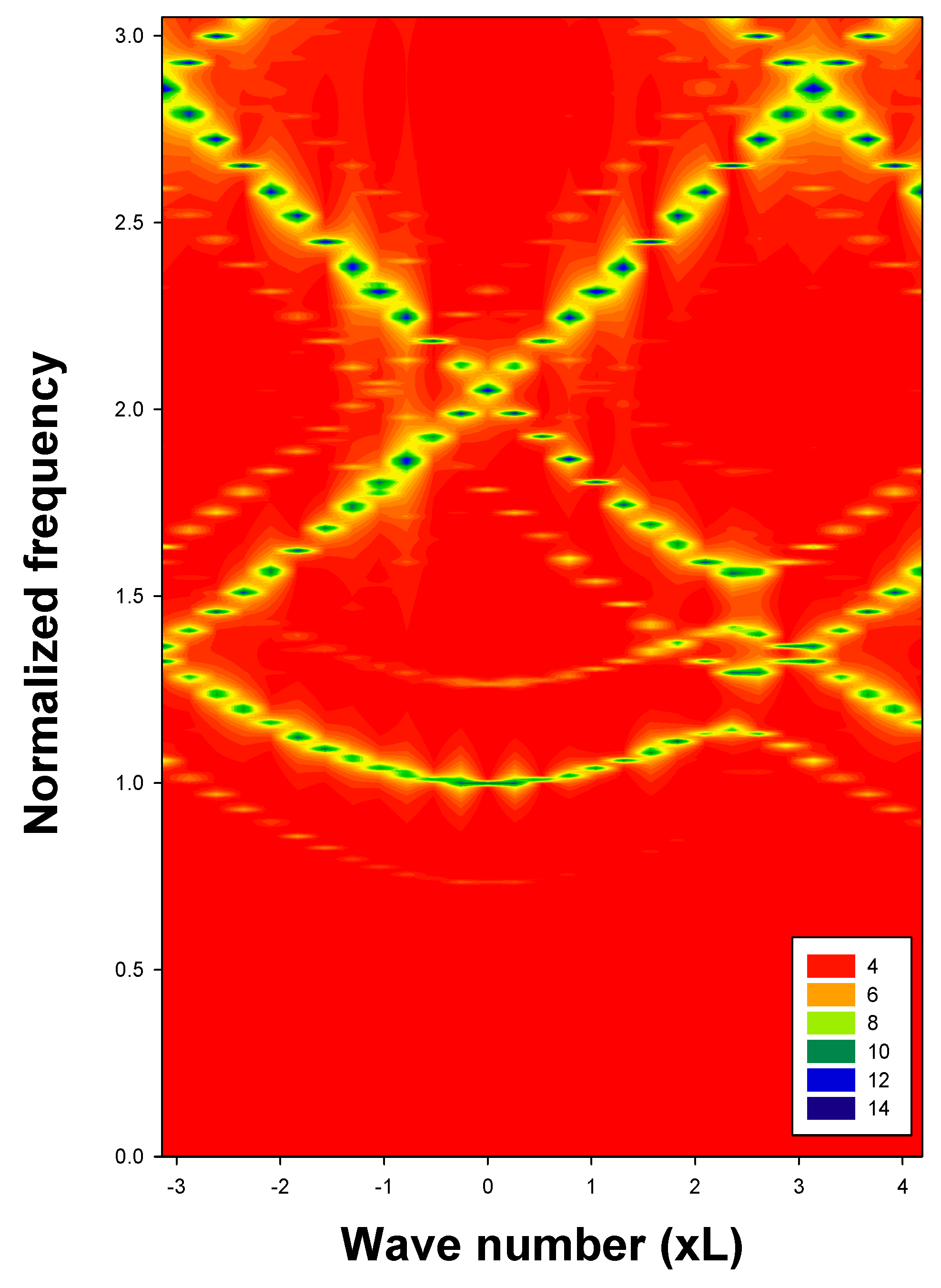To ensure adequate sampling of the system’s phase-space the SED calculations are averaged over 4 individual MD simulations, each simulation lasting 2²⁰ time steps and starting from randomly generated initial conditions. We report in Figure 5, the calculated band structure of the modulated system.

Figure 5 retains the essential features of the unperturbed band structure but for frequency shifted Bloch modes ${\omega }_0\left(k^{*}\right)\pm \mathsf{\Omega }$ and two band gaps in the positive half of the Brillouin zone. The periodicity of the band structure in wave number space is retained but its symmetry is broken. The frequency shifted modes are illustrative of the first-order particular solutions. Second-order frequency shifted modes ${\omega }_0\left(k^{*}\right)\pm 2\mathsf{\Omega }$ do not show in the figure due to their very weak amplitude. The two band gaps occur at the wave vector $k_{gap}$ defined by the condition ${\left({\omega }_0\left(k_{gap}+g\right)+\mathsf{\Omega }\right)}^2-{\omega }_0^2\left(k_{gap}+g-K\right)=0$ for g = 0 and g = K. It is the band folding due to the spatial modulation which enables overlap and hybridization between the frequency-shifted Bloch modes and the original Bloch modes of the lattice without the time dependency of the spatial modulation. The hybridization opens gaps in a band structure that has lost its mirror symmetry about the origin of the Brillouin zone. Considering the first gap and following a path in k space, starting at k = 0 at the bottom of the lowest branch, the wave function transitions from a state corresponding to a zeroth-order type wave, with orbital part ($e^{i{\omega }_0\left(k\right){\tau }_0}$) and spinor part $\left(\begin{array}{c}\sqrt{{\omega }_0+\beta k}\\ \sqrt{{\omega }_0-\beta k}\end{array}\right)$ to a wave having the characteristics of the first-order wave with orbital part ($e^{i\left({\omega }_0\left(k^{*}\right)-\mathsf{\Omega } \right){\tau }_0}$) and spinor part $\left(\begin{array}{c}{b}_1^{\prime }\\ b_2^{\prime }\end{array}\right)$. The control of the position of the gap through $\mathsf{\Omega }$ and K enables strategies for tuning the spinorial character of the elastic wave. The effect of these “spin-orbit” manipulations of the elastic system can be measured by examining the transmission of plane waves as shown in [4].

It is also instructive to consider the symmetry of the Dirac-like equations in the presence of a spatio-temporal modulation to best understand its effect on the spinorial character of the wave function. In the case of a modulation with a general phase φ, Equation (6a,b) take the overall form:

$$\left[{\sigma }_x\frac{\partial }{\partial t}+i\beta {\sigma }_y\frac{\partial }{\partial x}-i{\alpha }_{0}I-i{\alpha }_1\sin \left(Kx+\mathsf{\Omega }t+\phi \right)\right]\mathsf{\Psi }=0$$

(21a)

$$\left[{\sigma }_x\frac{\partial }{\partial t}+i\beta {\sigma }_y\frac{\partial }{\partial x}+i{\alpha }_{0}I+i{\alpha }_1\sin \left(Kx+\mathsf{\Omega }t+\phi \right)\right]\overline{\mathsf{\Psi }}=0$$

(21b)

Applying the joint T-symmetry and parity symmetry to Equation (21a) does not result in Equation (21b) for all phases φ but a few special values. The modulated Equations (21a,b) have lost the symmetry properties of the unmodulated Dirac equations Equation (6a,b). The gap that formed at $k_{gap}$ in Figure 4 is, therefore, not a Dirac point. The transformations $T_{\begin{array}{c}\omega \to \omega \\ k\to -k\end{array}}$ and $T_{\begin{array}{c}\omega \to -\omega \\ k\to k\end{array}}$ do not apply near $k_{gap}$. The constraints imposed on the spinorial component of the elastic wave function may be released in the vicinity of that wavenumber. This constraint was associated with Fermion-like wave functions which have the character of quasistanding waves, i.e., composed of forward and backward waves with a very specific proportion of their respective amplitudes. The release of the Dirac constraint associated with the impossibility for the medium to support forward propagating waves (+k_gap) but only backward propagating waves (−k_gap), may lead again to Boson-like behavior with no restriction on the amplitude of the backward propagating waves.

4. Conclusions

We presented phononic structures composed of two coupled one-dimensional harmonic chains and one harmonic chained grounded to a substrate that exhibit intrinsic non-conventional topology. This topology is associated with wave functions that possess spinorial and orbital components. The spinorial character of the wave function imparts a fermion-like character to the phonons. This behavior is reflected in a constraint on the amplitude of forward and backward going waves. We also developed a scalar Quantum Field Theory that demonstrates the analogy between the one-dimensional elastic system subjected to a spatio-temporal modulation of its elastic properties and the one-dimensional Dirac equation including an electromagnetic field. The directional spatio-temporal modulation enables the tuning of the spinorial and orbital components of the wave function. Since the spatio-temporal characteristics of the modulation are independent of each other they offer exquisite means of controlling the spinor components of the elastic wave. Practical physical realization of the modulation of elastic medium stiffness could be achieved by exploiting a variety of non-contact approaches including the photo-elastic effect [44], the magneto-elastic effect [45], and contact approaches such as the piezoelectric effect [46] or externally induced mechanical deformations [47]. The analogy between classical mechanical systems such as the ones demonstrated here and quantum and electromagnetic phenomena offer a new modality for developing more complex functions of phononic crystals and acoustic metamaterials. Such mechanical analogues of electromagnetic and quantum phenomena have a long history. For instance, Maxwell in his seminal paper “A dynamical theory of the electromagnetic field” [48] sought an elastic model of electrical and magnetic phenomena and electromagnetic waves. Other mechanical models of physical phenomena abound, including quantum mechanical behavior. For instance, the localization of ultrasound waves in two-dimensional [49] and three-dimensional [50] disordered phononic media serve as mechanical analogues of Anderson localization of electrons. Tunneling of classical waves through phononic crystal barriers establishes a correspondence with its quantum counterpart [51,52].

In addition to the mass spring systems reported in this paper, other physical systems that support elastic waves that can be described by Klein-Gordon-like equations include plates and phononic crystal plates [53], phononic crystals which support rotational elastic waves [5], granular phononic materials [54], elastic and sound wave guides with slowly varying cross sectional area [55].

Finally, we have addressed the topology of elastic wave functions and symmetry breaking in two linear 1-D mass-spring systems as well as in an extrinsic non-linear 1-D mass-spring system subjected to a spatio-temporal modulation of stiffness. More complex symmetry breaking conditions are expected to arise when considering intrinsic non-linear systems [56,57], such as for instance, phenomena associated with nonlinear resonances between linear and nonlinear systems. Indeed, coupled nonlinear and linear mechanical systems have recently received attention for their application in targeted energy transfer, whereby undesirable mechanical energy is directed irreversibly from a linear system to a nonlinear system [58].

References

1. Hasan, M.Z.; Kane, C.L. Colloquium: Topological insulators. Rev. Mod. Phys. 2010, 82, 3045. [Google Scholar] [CrossRef]
2. Khanikaev, A.B.; Mousavi, S.H.; Tse, W.-K.; Kargarian, M.; MacDonald, A.H.; Shvets, G. Photonic topological insulators. Nat. Mat. 2013, 12, 233–239. [Google Scholar] [CrossRef] [PubMed]
3. Haldane, F.D.M.; Raghu, S. Possible realization of directional optical waveguides in photonic crystals with broken time-reversal symmetry. Phys. Rev. Lett. 2008, 100, 013904. [Google Scholar] [CrossRef] [PubMed]
4. Deymier, P.A.; Runge, K.; Swinteck, N.; Muralidharan, K. Torsional topology and fermion-like behavior of elastic waves in phononic structures. Comptes Rendus Mécanique 2015, 343, 700–711. [Google Scholar] [CrossRef]
5. Deymier, P.A.; Runge, K.; Swinteck, N.; Muralidharan, K. Rotational modes in a phononic crystal with fermion-like behaviour. J. Appl. Phys. 2014, 115, 163510. [Google Scholar] [CrossRef]
6. Prodan, E.; Prodan, C. Topological phonon modes and their role in dynamic instability of microtubules. Phys. Rev. Lett. 2009, 103, 248101. [Google Scholar] [CrossRef] [PubMed]
7. Kane, C.L.; Lubensky, T.C. Topological boundary modes in isostatic lattices. Nat. Phys. 2013, 10, 39–45. [Google Scholar] [CrossRef]
8. Mousavi, S.; Khanikaev, A.B.; Wang, Z. Topologically protected elastic waves in phononic metamaterials. Nat. Commun. 2015, 6, 8682. [Google Scholar] [CrossRef] [PubMed]
9. Chen, B.G.; Upadhyaya, N.; Vitelli, V. Nonlinear conduction via solitons in a topological mechanical insulator. Proc. Natl. Acad. Sci. USA 2014, 111, 13004–13009. [Google Scholar] [CrossRef] [PubMed]
10. Süsstrunk, R.; Huber, S.D. Observation of phononic helical edge states in a mechanical topological insulator. Science 2015, 349, 47–50. [Google Scholar] [CrossRef] [PubMed]
11. Xiao, M.; Ma, G.; Yang, Z.; Sheng, P.; Zhang, Z.Q.; Chan, C.T. Geometric phase and band inversion in periodic acoustic systems. Nat. Phys. 2015, 11, 240–244. [Google Scholar] [CrossRef]
12. Paulose, J.; Chen, B.G.; Vitelli, V. Topological modes bound to dislocations in mechanical metamaterials. Nat. Phys. 2015, 11, 153–156. [Google Scholar] [CrossRef]
13. Berg, N.; Joel, K.; Koolyk, M.; Prodan, E. Topological phonon modes in filamentary structures. Phys. Rev. E 2011, 83, 021913. [Google Scholar] [CrossRef] [PubMed]
14. Pal, R.K.; Schaeffer, M.; Ruzzene, M. Helical edge states and topological phase transitions in phononic systems using bi-layered lattices. J. Appl. Phys. 2016, 119, 084305. [Google Scholar] [CrossRef]
15. Khanikaev, A.B.; Fleury, R.; Mousavi, S.H.; Alù, A. Topologically robust sound propagation in an angular-momentum-biased graphene-like resonator lattice. Nat. Commun. 2015, 6, 8260. [Google Scholar] [CrossRef] [PubMed]
16. Salerno, G.; Ozawa, T.; Price, H.M.; Carusotto, I. Floquet topological system based on frequency-modulated classical coupled harmonic oscillators. Phys. Rev. B 2015, 93, 085105. [Google Scholar] [CrossRef]
17. Paulose, J.; Meeussen, A.S.; Vitelli, V. Selective buckling via states of self-stress in topological metamaterials. Proc. Natl. Acad. Sci. USA 2015, 112, 7639–7644. [Google Scholar] [CrossRef] [PubMed]
18. Nash, L.M.; Kleckner, D.; Read, A.; Vitelli, V.; Turner, A.M.; Irvine, W.T.M. Topological mechanics of gyroscopic metamaterials. Proc. Natl. Acad. Sci. USA 2015, 112, 14495–14500. [Google Scholar] [CrossRef] [PubMed]
19. Wang, P.; Lu, L.; Bertoldi, K. Topological phononic crystals with one-way elastic edge waves. Phys. Rev. Lett. 2015, 115, 104302. [Google Scholar] [CrossRef] [PubMed]
20. Yang, Z.; Gao, F.; Shi, X.; Lin, X.; Gao, Z.; Chong, Y.; Zhang, B. Topological acoustics. Phys. Rev. Lett. 2015, 114, 114301. [Google Scholar] [CrossRef] [PubMed]
21. Unruh, W.G. Experimental black-hole evaporation? Phys. Rev. Lett. 1981, 46, 1351. [Google Scholar] [CrossRef]
22. Visser, M.; Molina-París, C. Acoustic geometry for general relativistic barotropic irrotational fluid flow. New J. Phys. 2010, 12, 095014. [Google Scholar] [CrossRef]
23. Bilic, N. Relativistic acoustics geometry. Class. Quantum Grav. 1999, 16, 3953–3964. [Google Scholar] [CrossRef]
24. Fleury, R.; Sounas, D.L.; Sieck, C.F.; Haberman, M.R.; Alu, A. Sound isolation and giant linear nonreciprocity in a compact acoustic circulator. Science 2014, 343, 516–519. [Google Scholar] [CrossRef] [PubMed]
25. Garcia de Andrade, L.C. Non-Riemannian geometry of vortex acoustics. Phys. Rev. D 2004, 70, 064004. [Google Scholar] [CrossRef]
26. Hoogstraten, H.W.; Kaper, B. Propagation of sound waves in a moving medium. J. Engr. Math. 1971, 5, 295–305. [Google Scholar] [CrossRef]
27. Godin, O.A. An exact wave equation for sound in inhomogeneous, moving, and non-stationary fluids. In Proceedings of the OCEANS′11 MTS/IEEE KONA, Waikoloa, HI, USA, 19–22 September 2011; pp. 1–5.
28. Wang, Q.; Yang, Y.; Ni, X.; Xu, Y.-L.; Sun, X.-C.; Chen, Z.-G.; Feng, L.; Liu, X.-P.; Lu, M.-H.; Chen, Y.-F. Acoustic asymmetric transmission based on time-dependent dynamical scattering. Nat. Sci. Rep. 2015, 5, 10880. [Google Scholar] [CrossRef] [PubMed]
29. Stone, M. Acoustic energy and momentum in a moving medium. Phys. Rev. E 2000, 62, 1341. [Google Scholar] [CrossRef]
30. Swinteck, N.; Matsuo, S.; Rung, K.; Vasseur, J.O.; Lucas, P.; Deymier, P.A. Bulk elastic waves with unidirectional backscattering-immune topological states in a time-dependent superlattice. J. Appl. Phys. 2015, 118, 063103. [Google Scholar] [CrossRef]
31. Berry, M.V. Quantal phase factors accompanying adiabatic changes. Proc. Roy. Soc. A 1984, 392, 45–57. [Google Scholar] [CrossRef]
32. Helleman, R.H.G.; Montroll, E.W. On a nonlinear perturbation theory without secular terms: I. classical coupled anharmonic oscillators. Physical 1974, 74, 22–74. [Google Scholar] [CrossRef]
33. Bender, C.M.; Orszag, S.A. Advanced Mathematical Methods for Scientists and Engineers I, Asymptotic Methods and Perturbation Theory; Springer-Verlag: New York, NY, USA, 1999. [Google Scholar]
34. Kevorkian, J.; Cole, J.D. Multiple Scale and Singular Perturbation Methods; Springer-Verlag: New York, NY, USA, 1996. [Google Scholar]
35. Belhaq, M.; Clerc, R.L.; Hartmann, C. Multiple scales methods for finding invariant solutions of two dimensional maps and application. Mech. Res. Commun. 1988, 15, 361. [Google Scholar] [CrossRef]
36. Maccari, A. A perturbation method for nonlinear two dimensional maps. Nonlinear Dynam. 1999, 19, 295–312. [Google Scholar] [CrossRef]
37. Van Horssen, W.T.; ter Brake, M.C. On the multiple scales perturbation method for difference equations. Nonlinear Dynam. 2009, 55, 401–408. [Google Scholar] [CrossRef]
38. Lee, P.S.; Lee, Y.C.; Chang, C.T. Multiple-time-scale analysis of spontaneous radiation processes. I. One- and Two-Particle Systems. Phys. Rev. A 1973, 8, 1722. [Google Scholar] [CrossRef]
39. Khoo, I.C.; Wang, Y.K. Multiple time scale analysis of an anharmonic crystal. J. Math. Phys. 1976, 17, 222. [Google Scholar] [CrossRef]
40. Swinteck, N.; Muralidharan, K.; Deymier, P.A. Phonon scattering in one-dimensional anharmonic crystals and superlattices: Analytical and numerical study. J. Vib. Acoust. ASME 2013, 135, 041016. [Google Scholar] [CrossRef]
41. Aharonov, Y.; Bohm, D. Significance of electromagnetic potentials in the quantum theory. Phys. Rev. 1959, 115, 485. [Google Scholar] [CrossRef]
42. Gupta, J.A.; Knobel, R.; Samarth, N.; Awschalom, D.D. Ultrafast manipulation of electron spin coherence. Science 2001, 292, 2458–2461. [Google Scholar] [CrossRef] [PubMed]
43. Thomas, J.A.; Turney, J.E.; Iutzi, R.M.; Amon, C.H.; McGaughey, A.J.H. Predicting phonon dispersion relations and lifetimes from the spectral energy density. Phys. Rev. B 2010, 81, 091411. [Google Scholar] [CrossRef]
44. Gump, J.; Finckler, I.; Xia, H.; Sooryakumar, R.; Bresser, W.J.; Boolchand, P. Light-induced giant softening of network glasses observed near the mean-field rigidity transition. Phys. Rev. Lett. 2004, 92, 245501. [Google Scholar] [CrossRef] [PubMed]
45. Bou-Matar, O.; Vasseur, J.O.; Hladky, A.-C.; Deymie, A. Band structures tunability of bulk 2D phononic crystals made of magneto-elastic materials. AIP Adv. 2011, 1, 041904. [Google Scholar]
46. Vasseur, J.O.; Hladky-Hennion, A.-C.; Djafari-Rouhani, B.; Duval, F.; Dubus, B.; Pennec, Y.; Deymier, P.A. Waveguiding in two-dimensional piezoelectric phononic crystal plates. J. Appl. Phys. 2007, 10, 114904. [Google Scholar] [CrossRef]
47. Rudykh, S.; Boyce, M.C. Transforming wave propagation in layered media via instability-induced interfacial wrinkling. Phys. Rev. Lett. 2014, 112, 034301. [Google Scholar] [CrossRef] [PubMed]
48. Maxwell, J.C. A dynamical theory of the electromagnetic field. Phil. Trans. R. Soc. Lond. 1865, 155, 459–512. [Google Scholar] [CrossRef]
49. Weaver, R.L. Localization of ultrasound. Wave Motion 1990, 12, 129–142. [Google Scholar] [CrossRef]
50. Hu, H.F.; Strybulevych, A.; Page, J.H.; Skipetrov, S.E.; Van Tiggelen, B.A. Localization of ultrasound in a three-dimensional elastic network. Nat. Phys. 2008, 4, 945–948. [Google Scholar] [CrossRef]
51. Van der Biest, F.; Sukhovich, A.; Tourin, A.; Page, J.H.; van Tiggelen, B.A.; Liu, Z.; Fink, M. Resonant tunneling of acoustic waves through a double barrier consisting of two phononic crystals. EPL 2005, 71, 63. [Google Scholar] [CrossRef]
52. Yang, S.; Page, J.H.; Zhengyou, L.; Cowan, M.L.; Chan, C.T.; Sheng, P. Ultrasound tunneling through 3D phononic crystals. Phys. Rev. Lett. 2002, 88, 104301. [Google Scholar] [CrossRef] [PubMed]
53. Vasseur, J.O.; Deymier, P.A.; Djafari-Rouhani, B.; Pennec, Y. Absolute forbidden bands in two-dimensional phononic crystal plates. Phys. Rev. B 2008, 77, 085415. [Google Scholar] [CrossRef]
54. Merkel, A.; Tournat, V.; Gusev, V. Experimental evidence of rotational elastic waves in granular phononic crystals. Phys. Rev. Lett. 2011, 107, 225502. [Google Scholar] [CrossRef] [PubMed]
55. Forbes, B.J.; Pike, E.R.; Sharp, D.B. The acoustical Klein-Gordon equation: The wave-mechanical step and barrier potential functions. J. Acoust. Soc. Am. 2003, 114, 1291–1302. [Google Scholar] [CrossRef] [PubMed]
56. Lazarov, B.S.; Jensen, J.S. Low-frequency band gaps in chains with attached non-linear oscillators. Int. J. Non-Linear Mech. 2007, 42, 1186–1193. [Google Scholar] [CrossRef]
57. Wang, Y.Z.; Li, F.M.; Wang, Y.S. Influences of active control on elastic wave propagation in a weakly nonlinear phononic crystal with a monoatomic lattice chain. Int. J. Mech. Sci. 2016, 106, 357–362. [Google Scholar] [CrossRef]
58. Vakakis, A.F.; Gendelman, O.V.; Bergman, L.A.; McFarland, D.M.; Kerschen, G.; Lee, Y.S. Nonlinear Targeted Energy Transfer in Mechanical and Structural Systems; Solid Mechanics and Its Application Series; Springer: Dordrecht, The Netherland, 2009. [Google Scholar]
Figure 1. Schematic illustration of the phononic structure composed of two coupled 1-D harmonic crystals. The atoms in the lower and upper 1-D harmonic crystals have mass m and M, respectively. The force constant of the springs of each 1-D harmonic crystal is taken to be the same, K0. The force constant of the coupling springs is KI. The periodicity of the crystal is a.
Crystals 06 00044 g001
Figure 2. Schematic illustration of the harmonic chain grounded to a substrate via side springs (system in Figure 1 when M ).
Crystals 06 00044 g002
Figure 3. Schematic representation of the manifold supporting Ψ and Ψ ¯ . The manifold exhibits a local quarter-turn twist around k = 0 of the square cross section of the manifold reflects the orthogonality of Ψ and Ψ ¯ . The clored arrows are parallel transported on the manifold along the direction of wave number. Their change in orientation is indicative of the phase change.
Crystals 06 00044 g003
Figure 4. Schematic illustration of the time evolution (top to bottom) of the harmonic chain grounded to a substrate with spatial modulation of the side spring stiffness illustrated as a “pink glow” of varying width when α > α 0 and a “blue glow” when α < α 0 .
Crystals 06 00044 g004
Figure 5. Band structure of the mechanical model system of Figure 2 calculated using the Spectral Energy Density (SED) method. The band structure is reported as a contour plot of the natural logarithm of the SED (color bar) versus normalized frequency and reduced wave number. The frequency is normalized to the lowest value of unperturbed band, namely 1.507 × 10⁵ Hz. The horizontal axis is extended to the right beyond the first Brillouin zone [−π,π] to highlight the asymmetry and therefore the modulation-induced symmetry breaking of the band structure. The brighter branches correspond to the usual zeroth-order type wave ( e i ω 0 ( k + g ) τ 0 ). The fainter branches parallel to the brighter ones are characteristic of first-order waves ( e i ( ω 0 ( k + g ) ± Ω   ) τ 0 ).
Crystals 06 00044 g005