Bound States and Supercriticality in Graphene-Based Topological Insulators

Abstract
1. Introduction
 exceeds (half of) the “Rashba” SOI
  . So far, the only 2D TIs realized experimentally are based on the mercury telluride class. Using graphene as a TI material constitutes a very attractive option because of the ready availability of high-quality graphene samples [1] and the exciting prospects for stable and robust TI-based devices [4], see also [12,13].
 , an additional mass term in the Hamiltonian corresponds to the intrinsic SOI (see below), and the massive Coulomb impurity problem in graphene has been analyzed in [21,22,23,24,25,26]. However, a finite Rashba SOI is inevitable in practice and has profound consequences. In particular,
  breaks electron-hole symmetry and modifies the structure of the vacuum. We therefore address the general case with both and finite, but within the TI phase
  , in this paper. Experimental progress on the observation of Dirac quasiparticles near a Coulomb impurity in graphene was also reported very recently [14], and we are confident that the topological version with enhanced SOI can be studied experimentally in the near future. Our work may also be helpful in the understanding of spin-orbit mediated spin relaxation in graphene [27].
 , could thereby be realized in topological graphene. Here we use the dimensionless impurity strength
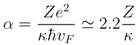
 is the number of positive charges held by the impurity;
  a dielectric constant characterizing the environment; and
  m
m  s the Fermi velocity. Without SOI, the Hamiltonian is not self-adjoint for
  , and the potential needs short-distance regularization, e.g., by setting
  with short-distance cutoff
  of the order of the lattice constant of graphene [1,2]. Including a finite “mass” , i.e., the intrinsic SOI, but keeping , the critical coupling
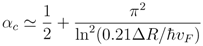
  is shifted to [24]
 for
for  . In the supercritical regime
  , the lowest bound state “dives” into the valence band continuum (Dirac sea). It then becomes a resonance with complex energy, where the imaginary part corresponds to the finite decay rate into the continuum. Below we show that the Rashba SOI provides an interesting twist to this supercriticality story. The structure of this article is as follows. In Section 2 we introduce the model and summarize its symmetries. The case of a circular potential well is addressed in Section 3 before turning to the Coulomb center in Section 4. Some conclusions are offered in Section 5. Note that we do not include a magnetic field (see, e.g., [28,29]) and thus our model enjoys time-reversal symmetry. Below, we often use units with
  .
.2. Model and Symmetries
2.1. Kane–Mele Model with Radially Symmetric Potential
) and Rashba ( ) SOI [3] in the presence of a radially symmetric scalar potential  . Assuming that is sufficiently smooth to allow for the neglect of inter-valley scattering, the low-energy Hamiltonian near the
  point
point  is given by

 (
(  ) in sublattice (spin) space [1]. The Hamiltonian near the other valley (
  point) follows for
  in Equation (3). We note that a sign change of the Rashba SOI,
  , does not affect the spectrum due to the relation
  . Without loss of generality, we then put
  and
and  .
.
 . For given , eigenfunctions of
  must then be of the form
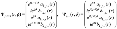
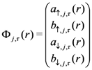 and valley index
  reads
reads
 denotes the intrinsic SOI and not the Laplacian)
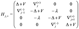
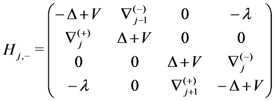


 , spin and sublattice are flipped simultaneously, and only the
  -coordinate is reversed. (We will nonetheless refer to as parity transformation below.) A second symmetry relation connects both valleys,
 , the current density operator has angular component
  and radial component
  for arbitrary . When real-valued entries can be chosen in
  , the radial current density thus vanishes separately in each valley. We define the (angular) spin current density as
  . Remarkably, the transformation defined in Equation (11) conserves both (total and spin) angular currents, while the transformation in Equation (10) reverses the total current but conserves the spin current. Therefore, at any energy, eigenstates supporting spin-filtered counterpropagating currents are possible. However, in contrast to the edge states found in a ribbon geometry [3], these spin-filtered states do not necessarily have a topological origin. point (
  ) and omit the
  -index henceforth; the degenerate
  Kramers partner easily follows using Equation (11). In addition, using the symmetry (10), it is sufficient to study the model for fixed total angular momentum
  .
.2.2. Zero Total Angular Momentum
, we now show that a drastic simplification is possible for total angular momentum  , which can even allow for an exact solution. Although the lowest-lying bound states for the potentials in Section 3 and Section 4 are found in the
  sector, exact statements about what happens for are valuable and can be explored along the route sketched here. is special can be seen from the parity symmetry relation in Equation (10). The parity transformation connects the
  sectors, but represents a discrete symmetry of the radial Hamiltonian
  [see Equation (8)] acting on the four-spinors in Equation (6). Therefore, the subspace can be decomposed into two orthogonal subspaces corresponding to the two distinct eigenvalues of the Hermitian operator . This operator is diagonalized by the matrix
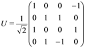

 , we obtain
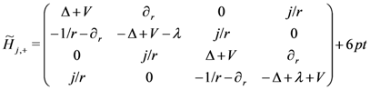 , the upper and lower
  blocks decouple. Each block has the signature (“parity”)
  corresponding to the eigenvalues in Equation (13), and represents a mixed sublattice-spin state, see Equations (6) and (12)., the block matrix in Equation (14) is formally identical to an effective problem with , fixed
  , and the substitutions
 and arbitrary , the complete spectral information for the full Kane–Mele problem (with ) directly follows from the solution.
2.3. Solution in Region with Constant Potential
 , since
  and
and  enter only through the combination
  in Equation (8). In Section 3, we will use this solution to solve the case of a step potential.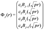
 are real coefficients;
  is one of the cylinder (Bessel) functions;
  or
or  ; and
; and  denotes a real spectral parameter. In particular,
  is a generalized radial wavenumber. We here assume true bound-state solutions with real-valued energy. However, for quasi-stationary resonance states with complex energy, and the may be complex as well.
 , the set of four coupled differential Equations (7) simplifies to a set of algebraic equations
 does not appear here, and therefore the spectral parameter depends only on the energy . The condition of vanishing determinant then yields a quadratic equation for , with the two solutions

 and on the imposed regularity conditions for
  and/or
  .
. , a solution regular at the origin is obtained by putting , which describes standing radial waves. Equation (17) then yields the unnormalized spinor
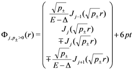
 , instead it is convenient to set in Equation (16). Using the identity
  , the unnormalized spinor resulting from Equation (17) then takes the form
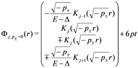
 describes evanescent modes, exponentially decaying at infinity.
2.4. Solution without Potential
for all  , the only acceptable solution corresponding to a physical state is obtained when [30]. For
  , at least one in Equation (18) for all , and the system is gapless. However, the TI phase defined by has a gap as we show now., Equation (18) tells us that for
  and for
  , both solutions are positive and hence (for given and ) there are two eigenstates
  for given energy . However, within the energy window [with
  in Equation (18)]

 and
and  , i.e., only the eigenstate
  represents a physical solution. Both are negative when
  , and no physical state exists at all. This precisely corresponds to the topological gap in the TI phase [3]. Note that due to the Rashba SOI, the valence band edge is characterized by the two energies , with halved density of states in the energy window (21). One may then ask at which energy (
  or
or  ) the supercritical diving of a bound state level in an impurity potential takes place.
 3. Circular Potential Well
3.1. Bound States
and depth 
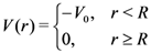 , where bound states are expected for energies
  in the window
  . For
. For  , the corresponding radial eigenspinor [see Equation (6)] is written with arbitrary prefactors
  in the form
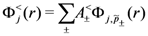
 . Here, the
  follow from Equation (18) by including the potential shift,

 , the general solution is again written as
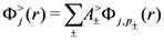 is given by Equation (20), since for true bound states with only evanescent states outside the potential well.
 then yields a homogeneous linear system of equations for the four parameters (
  ). A nontrivial solution is only possible when the determinant of the corresponding
  matrix
  (which is too lengthy to be given here but follows directly from the above expressions) vanishes

 ). It is then straightforward to determine the corresponding spinor wavefunctions.
 exceeds a ( -dependent) “threshold” value,
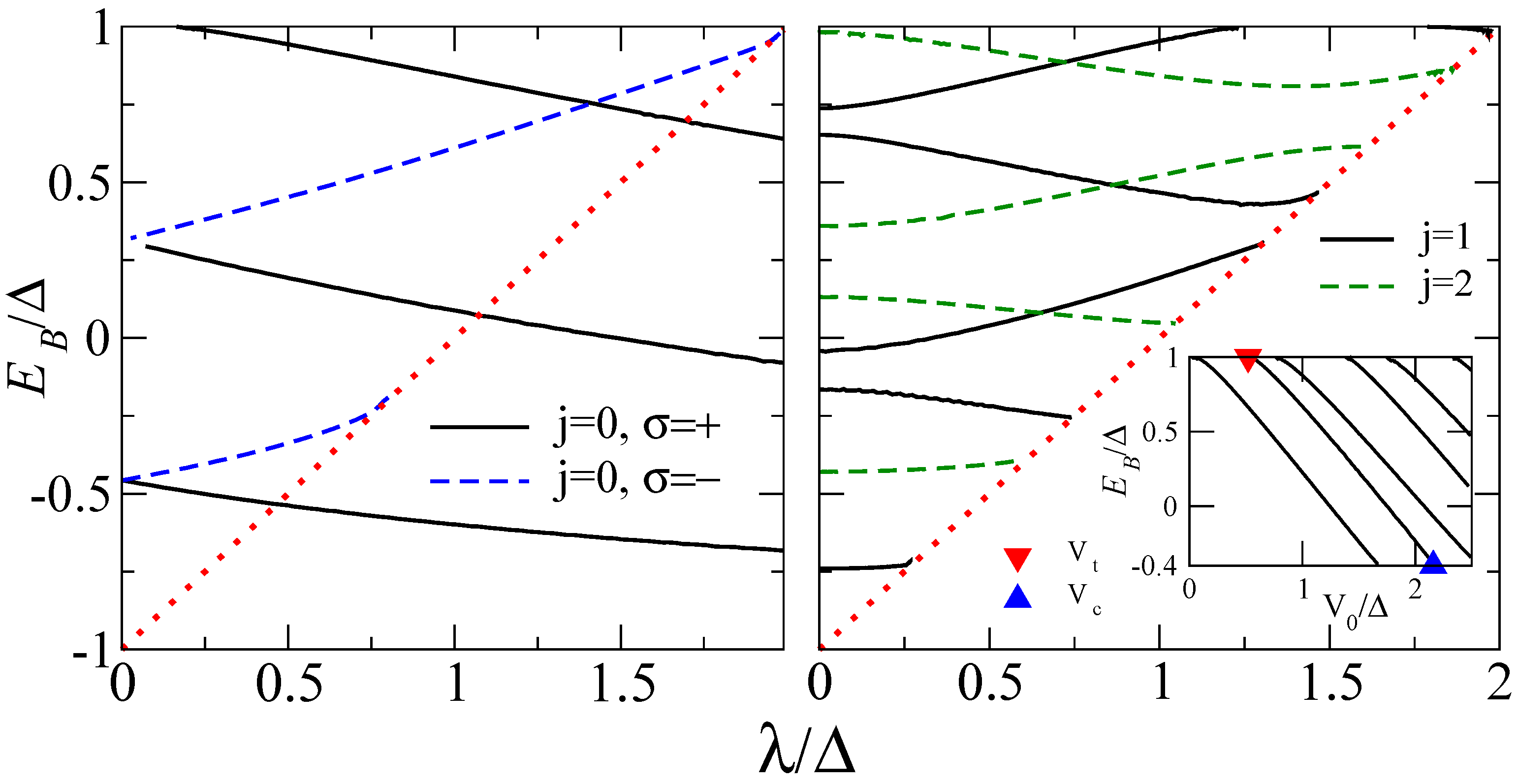
  , a bound state splits off the conduction band edge. When increasing further, this bound-state energy level moves down almost linearly, cf. inset of Figure 1, and finally reaches the valence band edge
  at some “critical” value
  . (For , we will see below that this definition needs some revision.) Increasing even further, the bound state is then expected to dive into the valence band and become a finite-width supercritical resonance, i.e., the energy would then acquire an imaginary part.) vs. Rashba SOI ( ) for a circular potential well with depth
  and radius
  . Only the lowest-energy states with
  are shown. The red dotted line indicates . The left panel shows bound states with parity . The right panel shows
  bound states. The inset displays the bound-state energies vs. potential depth for
  . At some threshold value
  (where
  for the lowest state shown), a new bound state emerges from the conduction band. This state dives into the valence band for some critical value
  , where the valence band edge is at energy
 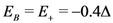 . For the second bound state in the inset, (
  ) is shown as red (blue) triangle.
) vs. Rashba SOI ( ) for a circular potential well with depth and radius . Only the lowest-energy states with are shown. The red dotted line indicates . The left panel shows bound states with parity . The right panel shows bound states. The inset displays the bound-state energies vs. potential depth for . At some threshold value (where for the lowest state shown), a new bound state emerges from the conduction band. This state dives into the valence band for some critical value , where the valence band edge is at energy . For the second bound state in the inset, ( ) is shown as red (blue) triangle.
) is shown as red (blue) triangle.
) vs. Rashba SOI ( ) for a circular potential well with depth and radius . Only the lowest-energy states with are shown. The red dotted line indicates . The left panel shows bound states with parity . The right panel shows bound states. The inset displays the bound-state energies vs. potential depth for . At some threshold value (where for the lowest state shown), a new bound state emerges from the conduction band. This state dives into the valence band for some critical value , where the valence band edge is at energy . For the second bound state in the inset, ( ) is shown as red (blue) triangle. 
3.2. Zero Angular Momentum States
, we find a different scenario where supercritical diving, with finite lifetime of the resonance, happens only for half of the bound states entering the energy window (21). Noting that states with different parity do not mix, see Section 2.2, we observe that all  bound states enter the valence band as true bound states (no imaginary part) throughout the energy window (21) while the valence band continuum is spanned by the
  states. We then define for
  bound states as the true supercritical threshold where
  . However, the
  bound states become supercritical already when reaching . in the energy window (21). While states are true bound states (no lifetime broadening), they coexist with states which span the valence band continuum or possibly form supercritical resonances. For , however, all bound states dive, become finite-width resonances, and eventually become dissolved in the continuum.
3.3. Threshold for Bound States
, we observe that whenever hits a possible threshold value , a new bound state is generated, which then dives into the valence band at another potential depth (and so on). Analytical results for all possible threshold values follow by expanding Equation (26) for weak dimensionless binding energy  For
For  and , Equation (26) yields after some algebra


 is the Euler constant and
  . The binding energy approaches zero for
  , where Equation (27) simplifies to
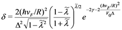 , this reproduces known results [25]. For any
  , we observe that the bound state in Equation (28) exists for arbitrarily shallow potential depth . for higher-lying bound states also follow from the binding energy (27), since
  vanishes for
  and for
  . When one of these two conditions is fulfilled at some , a new bound state appears for potential depth above . This statement is in fact quite general: By similar reasoning, we find that the threshold values for follow by counting the zeroes of
  . Without SOI, this has also been discussed in [31]. Note that this argument immediately implies that no bound state with exists for . for all bound states with or in analytical form. These are labeled by
  and (for ,
  corresponds to parity)

 is the
  th zero of the
  Bessel function.
 , the condition for the appearance of a new bound state is
 exist for . We conclude that bound states in a very weak potential well exist only for .
3.4. Supercritical Behavior
bound state is also the first to enter the valence band continuum for . For , the critical value is known to be [25]

 . The energy of the resonant state acquires an imaginary part for
  [25]. For
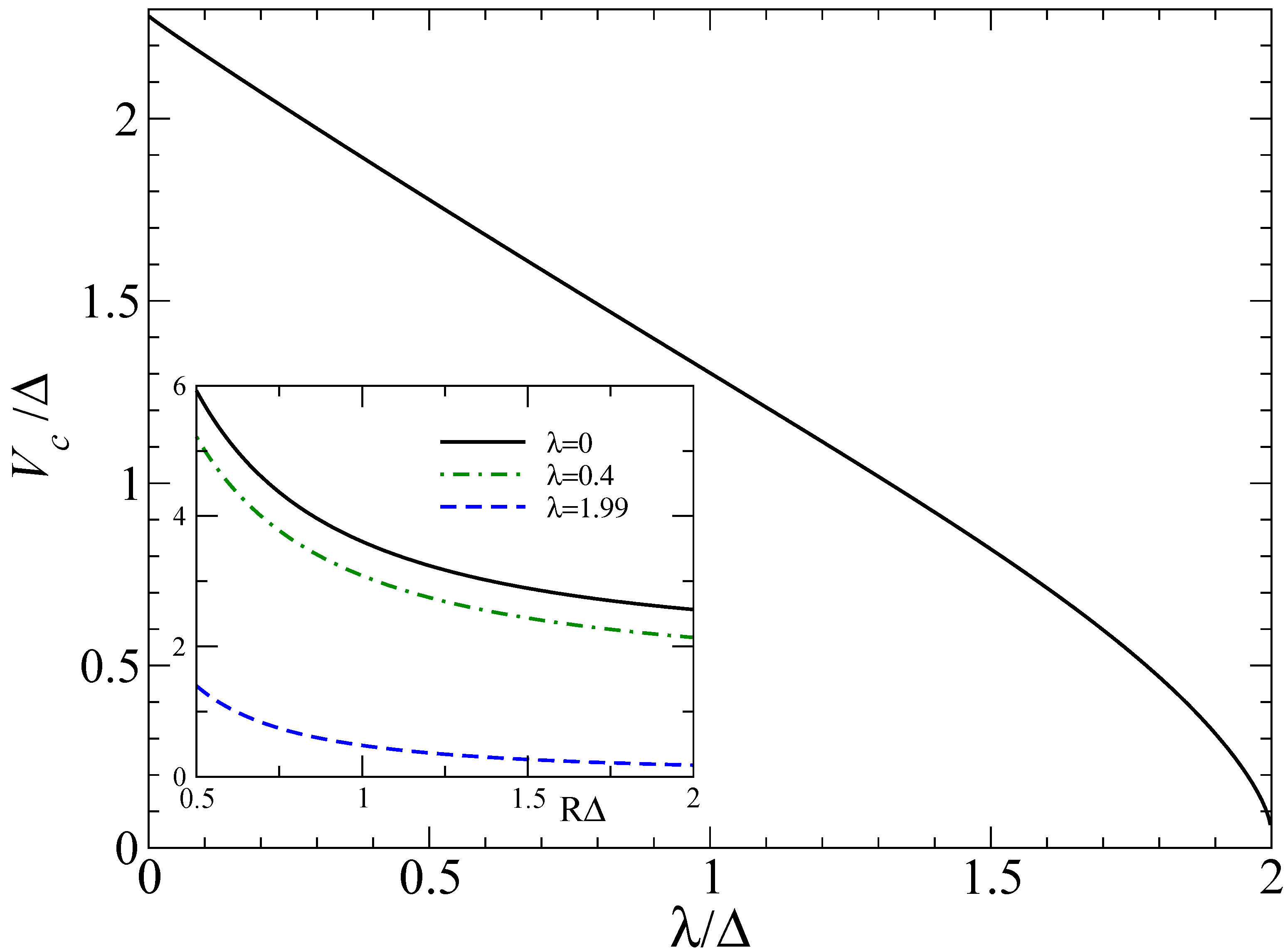
  , we have obtained implicit expressions for , plotted in Figure 2. Note that these results reproduce Equation (31) for
  . The almost linear decrease of with increasing , see Figure 2, can be rationalized by noting that the valence band edge is located at . Thereby supercritical resonances could be reached already for lower potential depth by increasing the Rashba SOI. Similarly, with increasing disk radius , the critical value decreases, see the inset of Figure 2. For the lowest
  bound state, the critical value in fact follows in analytical form,

 . for the lowest bound state level in a disk with
  . The obtained value matches the analytical prediction
  from Equation (31), while
  near the border of the TI phase (
  ). Inset: vs. radius with several values of (given in units of ) for the lowest bound state.
for the lowest bound state level in a disk with . The obtained value matches the analytical prediction from Equation (31), while near the border of the TI phase ( ). Inset: vs. radius with several values of (given in units of ) for the lowest bound state.
). Inset: vs. radius with several values of (given in units of ) for the lowest bound state.
for the lowest bound state level in a disk with . The obtained value matches the analytical prediction from Equation (31), while near the border of the TI phase ( ). Inset: vs. radius with several values of (given in units of ) for the lowest bound state.  , it is natural to expect that all
  bound states turn into finite-width resonances when
  . This expectation is confirmed by an explicit calculation as follows. Within in the window
  , a true bound state should not receive a contribution from
  for , but instead has to be obtained by matching an Ansatz as in Equation (23) for the spinor state inside the disk ( ) to an evanescent spinor state
  . However, the matching condition is then found to have no real solution , i.e., there are no true bound states with in the energy window (21). We therefore conclude that all bound states turn supercritical when . Note that this statement includes the lowest-lying bound state (which has ). This implies that a finite Rashba SOI can considerably lower the potential depth required for entering the supercritical regime.
4. Coulomb Center
 , generated by a positively charged impurity located at the origin, with the dimensionless coupling strength
  in Equation (1). We consider only the TI phase and analyze the bound-state spectrum and conditions for supercriticality. Again, without loss of generality, we focus on the point only ( ), and first summarize the known solution for [2,21,24]. In that case,
  is conserved, and the spin-degenerate bound-state energies are labeled by the integer angular momentum and a radial quantum number
  (for
(for  ,
,  is also possible)
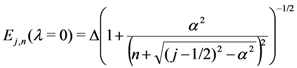
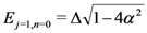 , which dives when
  ; note that precisely corresponds to in Section 3. In particular, for (
  states we define in the same manner. Next we discuss how this picture is modified when the Rashba coupling is included., the combination of Equation (33) with Equation (15) immediately yields the exact bound-state energy spectrum ( )

 potential [23,24], where
  is replaced by the constant value
  . Here, is a short-distance cutoff scale of the order of the lattice spacing. The solution of the bound-state problem then requires a wavefunction matching procedure, which has been carried out in [24]. Thereby we can already infer all bound states for . bound-state spectrum vs. for the regularized Coulomb potential. Within the energy window Equation (21), we again find that states with parity remain true bound states that dive only for
  , while states show supercritical diving already for . Figure 4 shows the corresponding critical couplings for , where the lowest bound state with parity turns supercritical. Note that for finite and , a unique value for is found, while for two different critical values for are found. However, this conclusion holds only for finite regularization parameter , i.e., it is non-universal. As seen in the inset of Figure 4, in the limit , both critical values for approach again, which is the value found without SOI., we can then draw the same qualitative conclusions as in Section 3.4 for the potential well. In particular, we expect that all bound states turn supercritical when their energy reaches the continuum threshold at
  . ( in units of ) vs. dimensionless impurity strength for the Coulomb problem with regularization parameter
  and Rashba SOI . Solid black (dashed blue) curves correspond to parity ( ). Results for radial number
  (with increasing energy) are shown. Red dotted lines denote
  .
( in units of ) vs. dimensionless impurity strength for the Coulomb problem with regularization parameter and Rashba SOI . Solid black (dashed blue) curves correspond to parity ( ). Results for radial number (with increasing energy) are shown. Red dotted lines denote .
.
( in units of ) vs. dimensionless impurity strength for the Coulomb problem with regularization parameter and Rashba SOI . Solid black (dashed blue) curves correspond to parity ( ). Results for radial number (with increasing energy) are shown. Red dotted lines denote . 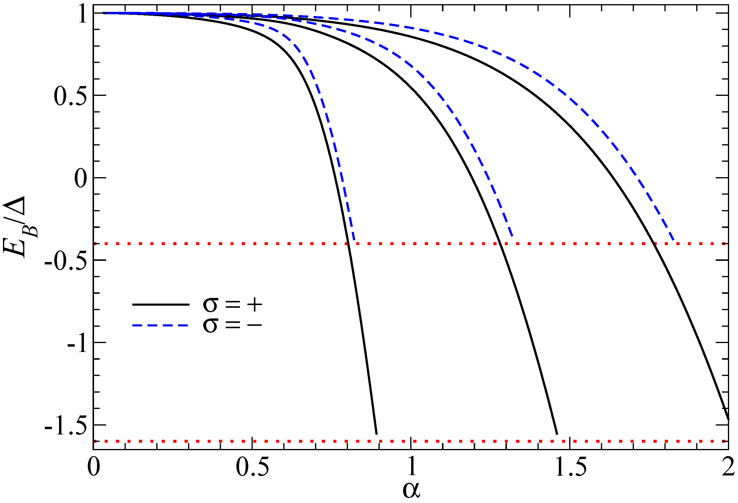 vs. Rashba SOI for and the lowest bound states. Inset: vs. cutoff scale for .
vs. Rashba SOI for and the lowest bound states. Inset: vs. cutoff scale for .
vs. Rashba SOI for and the lowest bound states. Inset: vs. cutoff scale for .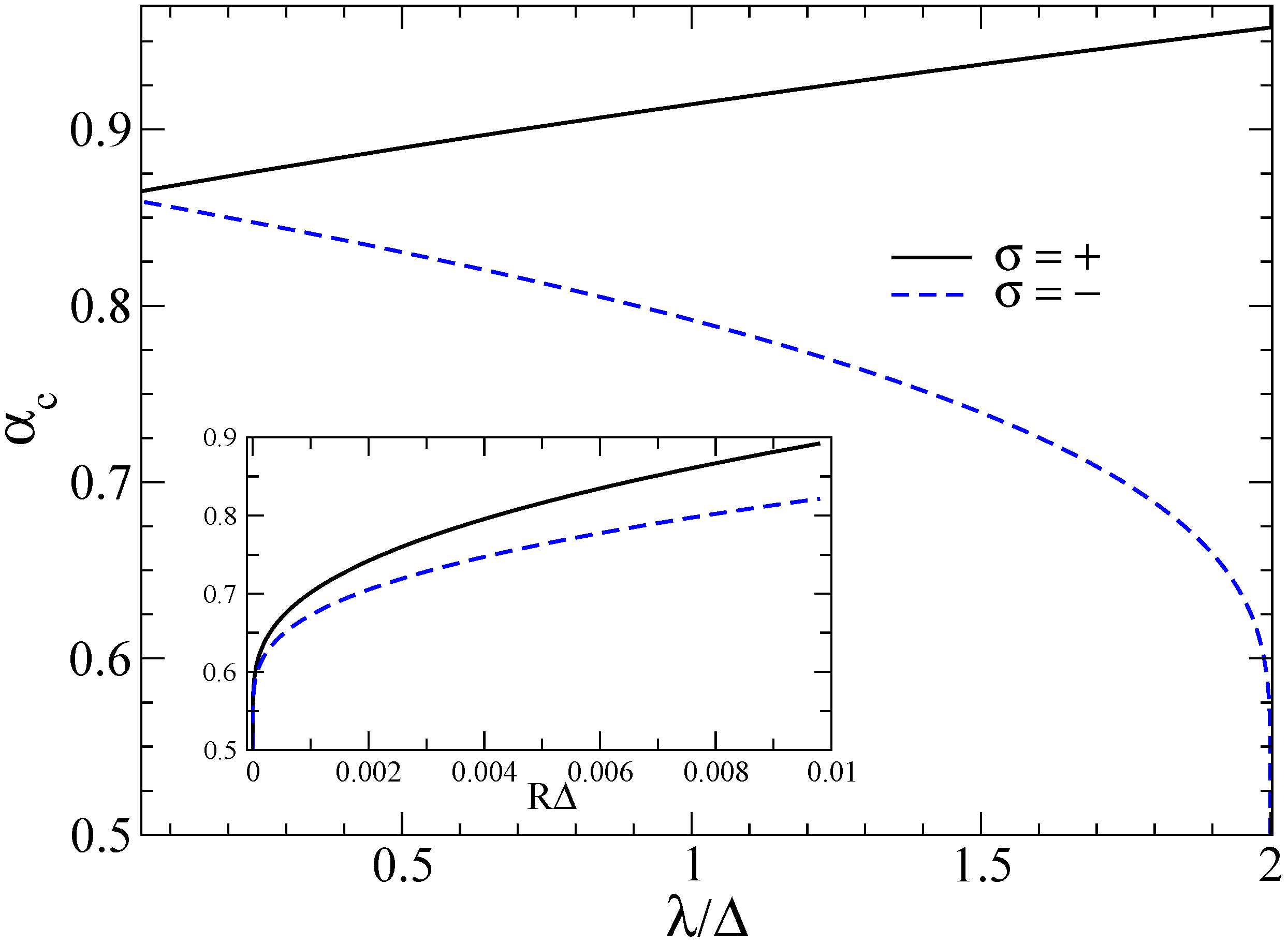
5. Conclusions
) and Rashba ( ) spin-orbit couplings when a radially symmetric attractive potential is present. We have focused on the most interesting “topological insulator” phase with . The Rashba term leads to a restructuring of the valence band, with a halving of the density of states in the window  , where
  . This has spectacular consequences for total angular momentum , where the problem can be decomposed into two independent parity sectors ( ). The states remain true bound states even inside the above window and coexist with the continuum solutions as well as possible supercritical resonances in the sector. However, all bound states exhibit supercritical diving for
  , where the critical threshold ( or for the disk or the Coulomb problem, respectively) is lowered when the Rashba term is present. We hope that these results will soon be put to an experimental test.
Acknowledgements
References
- Castro Neto, A.H.; Guinea, F.; Peres, N.M.R.; Novoselov, K.S.; Geim, A. The electronic properties of graphene. Rev. Mod. Phys. 2009, 81, 109–162. [Google Scholar] [CrossRef]
- Kotov, V.N.; Uchoa, B.; Pereira, V.M.; Guinea, F.; Castro Neto, A.H. Electron-electron interactions in graphene: Current status and perspectives. Rev. Mod. Phys. 2012, 84, 1067–1125. [Google Scholar] [CrossRef]
- Kane, C.L.; Mele, E.J. Quantum spin hall effect in graphene. Phys. Rev. Lett. 2005, 95, 226801:1–226801:4. [Google Scholar]
- Hasan, M.Z.; Kane, C.L. Topological insulators. Rev. Mod. Phys. 2010, 82, 3045–3067. [Google Scholar] [CrossRef]
- Huertas-Hernando, D.; Guinea, F.; Brataas, A. Spin-orbit coupling in curved graphene, fullerenes, nanotubes, and nanotube caps. Phys. Rev. B 2006, 74, 155426:1–155426:15. [Google Scholar]
- Min, H.; Hill, J.E.; Sinitsyn, N.A.; Sahu, B.R.; Kleinman, L.; MacDonald, A.H. Intrinsic and Rashba spin-orbit interactions in graphene sheets. Phys. Rev. B 2006, 74, 165310:1–165310:5. [Google Scholar]
- Yao, Y.; Ye, F.; Qi, X.L.; Zhang, S.C.; Fang, Z. Spin-orbit gap of graphene: First-principles calculations. Phys. Rev. B 2007, 75, 041401(R):1–041401(R):4. [Google Scholar]
- Weeks, C.; Hu, J.; Alicea, J.; Franz, M.; Wu, R. Engineering a robust quantum spin hall state in graphene via adatom deposition. Phys. Rev. X 2011, 1, 021001:1–021001:15. [Google Scholar]
- Shevtsov, O.; Carmier, P.; Groth, C.; Waintal, X.; Carpentier, D. Graphene-based heterojunction between two topological insulators. Phys. Rev. X 2012, 2, 031004:1–031004:10. [Google Scholar]
- Shevtsov, O.; Carmier, P.; Groth, C.; Waintal, X.; Carpentier, D. Tunable thermopower in a graphene-based topological insulator. Phys. Rev. B 2012, 85, 245441:1–245441:7. [Google Scholar]
- Jiang, H.; Qiao, Z.; Liu, H.; Shi, J.; Niu, Q. Stabilizing topological phases in graphene via random adsorption. Phys. Rev. Lett. 2012, 109, 116803:1–116803:5. [Google Scholar]
- Bercioux, D.; de Martino, A. Spin-resolved scattering through spin-orbit nanostructures in graphene. Phys. Rev. B 2010, 81, 165410:1–165410:9. [Google Scholar] [CrossRef]
- Lenz, L.; Bercioux, D. Dirac-Weyl electrons in a periodic spin-orbit potential. Europhys. Lett. 2011, 96, 27006:1–27006:6. [Google Scholar]
- Wang, Y.; Brar, V.W.; Shytov, A.V.; Wu, Q.; Regan, W.; Tsai, H.Z.; Zettl, A.; Levitov, L.S.; Crommie, M.F. Mapping dirac quasiparticles near a single coulomb impurity on graphene. Nat. Phys. 2012, 8, 653–657. [Google Scholar] [CrossRef]
- Katsnelson, M.I. Nonlinear screening of charge impurities in graphene. Phys. Rev. B 2006, 74, 201401(R):1–201401(R):3. [Google Scholar]
- Pereira, V.M.; Nilsson, J.; Castro Neto, A.H. Coulomb impurity problem in graphene. Phys. Rev. Lett. 2007, 99, 166802:1–166802:4. [Google Scholar]
- Shytov, A.V.; Katsnelson, M.I.; Levitov, L.S. Vacuum polarization and screening of supercritical impurities in graphene. Phys. Rev. Lett. 2007, 99, 236801:1–236801:5. [Google Scholar]
- Shytov, A.V.; Katsnelson, M.I.; Levitov, L.S. Atomic collapse and quasi-rydberg states in graphene. Phys. Rev. Lett. 2007, 99, 246802:1–246802:5. [Google Scholar]
- Biswas, R.R.; Sachdev, S.; Son, D.T. Coulomb impurity in graphene. Phys. Rev. B 2007, 76, 205122:1–205122:5. [Google Scholar]
- Fogler, M.M.; Novikov, D.S.; Shklovskii, B.I. Screening of a hypercritical charge in graphene. Phys. Rev. B 2007, 76, 233402:1–233402:4. [Google Scholar]
- Novikov, D.S. Elastic scattering theory and transport in graphene. Phys. Rev. B 2007, 76, 245435:1–245435:17. [Google Scholar]
- Terekhov, I.S.; Milstein, A.I.; Kotov, V.I.; Sushkov, O.P. Screening of coulomb impurities in graphene. Phys. Rev. Lett. 2008, 100, 076803:1–076803:4. [Google Scholar]
- Pereira, V.M.; Kotov, V.N.; Castro Neto, A.H. Supercriticial coulomb impurities in gapped graphene. Phys. Rev. B 2008, 78, 085101:1–085101:8. [Google Scholar]
- Gamayun, O.B.; Gorbar, E.V.; Gusynin, V.P. Supercritical coulomb center and excitonic instability in graphene. Phys. Rev. B 2009, 80, 165429:1–165429:14. [Google Scholar]
- Gamayun, O.B.; Gorbar, E.V.; Gusynin, V.P. Magnetic field driven instability of a charged center in graphene. Phys. Rev. B 2011, 83, 235104:1–235104:9. [Google Scholar]
- Zhu, J.L.; Sun, S.; Yang, N. Dirac donor states controlled by magnetic field in gapless and gapped graphene. Phys. Rev. B 2012, 85, 035429:1–035429:9. [Google Scholar]
- Huertas-Hernando, D.; Guinea, F.; Brataas, A. Spin-orbit mediated spin relaxation in graphene. Phys. Rev. Lett. 2009, 103, 146801:1–146801:4. [Google Scholar]
- Rashba, E.I. Graphene with structure-induced spin-orbit coupling: Spin-polarized states, spin zero modes, and quantum Hall effect. Phys. Rev. B 2009, 79, 161409(R):1–161409(R):4. [Google Scholar]
- De Martino, A.; Hütten, A.; Egger, R. Landau levels, edge states, and strained magnetic waveguides in graphene monolayers with enhanced spin-orbit interaction. Phys. Rev. B 2011, 84, 155420:1–155420:12. [Google Scholar]
- Rakyta, P.; Kormanyos, A.; Cserti, J. Trigonal warping and anisotropic band splitting in monolayer graphene due to Rashba spin-orbit coupling. Phys. Rev. B 2010, 82, 113405:1–113405:4. [Google Scholar]
- Bardarson, J.H.; Titov, M.; Brouwer, P.W. Electrostatic confinement of electrons in an integrable graphene quantum dot. Phys. Rev. Lett. 2009, 102, 226803:1–226803:4. [Google Scholar]
© 2013 by the authors; licensee MDPI, Basel, Switzerland. This article is an open-access article distributed under the terms and conditions of the Creative Commons Attribution license (http://creativecommons.org/licenses/by/3.0/).
Share and Cite
Klöpfer, D.; De Martino, A.; Egger, R. Bound States and Supercriticality in Graphene-Based Topological Insulators. Crystals 2013, 3, 14-27. https://doi.org/10.3390/cryst3010014
Klöpfer D, De Martino A, Egger R. Bound States and Supercriticality in Graphene-Based Topological Insulators. Crystals. 2013; 3(1):14-27. https://doi.org/10.3390/cryst3010014
Chicago/Turabian StyleKlöpfer, Denis, Alessandro De Martino, and Reinhold Egger. 2013. "Bound States and Supercriticality in Graphene-Based Topological Insulators" Crystals 3, no. 1: 14-27. https://doi.org/10.3390/cryst3010014
APA StyleKlöpfer, D., De Martino, A., & Egger, R. (2013). Bound States and Supercriticality in Graphene-Based Topological Insulators. Crystals, 3(1), 14-27. https://doi.org/10.3390/cryst3010014