Stable Sampling Equilibrium in Common Pool Resource Games

Abstract

This paper reconsiders evidence from experimental common pool resource games from the perspective of a model of payoff sampling. Despite being parameter-free, the model is able to replicate some striking features of the data, including single-peaked frequency distributions, the persistent use of strictly dominated actionsand stable heterogeneity in choices. These properties can also be accurately replicated using logit quantal response equilibrium (QRE), but only by tuning the free parameter separately for separate games. When the QRE parameter is constrained to be the same across games, sampling equilibrium provides a superior fit to the data. We argue that these findings are likely to generalize to other complex games with multiple players and strategies.

1. Introduction

Common property is a regime involving a well-defined set of users, each of whom has rights to the extraction of an economically-valuable resource. Many inshore fisheries, grazing lands, forest areas and water resources are accessed under these conditions. The notion that such resources could be exploited in a manner that is sustainable and reasonably efficient is supported by numerous case studies, as well as theoretical models and experimental tests using subjects in the lab and the field. 1

Experimental studies of common pool resource games have generally followed the protocol introduced by Ostrom et al. [3,4]. These experiments involve a finite number of rounds in which subjects take actions intended to mimic the extraction of a resource held as common property. This involves a negative externality, since higher levels of extraction reduce the marginal returns to the extractive effort of all players. Standard equilibrium analysis predicts over-extraction of the resource relative to efficient levels under these conditions.

The behavior of subjects in common pool resource experiments typically deviates substantially from this equilibrium prediction in a number of interesting respects. All available actions are chosen with a positive frequency, with strictly dominated actions being chosen persistently and often. The frequency distribution has a structure where levels of extraction that are less individually costly are selected more often. Average extraction is relatively stable over time, lying below equilibrium levels, but above efficient levels.

We argue in this paper that these patterns can be accurately replicated with a model of payoff sampling equilibrium (PSE) introduced by Osborne and Rubinstein [7], subject to a suitable refinement. The basic idea underlying this solution concept is that individuals try out multiple actions, observe payoffs and subsequently adopt actions that were the most rewarding. A sampling equilibrium is a distribution of actions in a population that reproduces itself, in the sense that the likelihood with which an action is selected under the sampling procedure matches the frequency with which it is currently being used.

While a PSE can involve the play of strictly dominated strategies with positive probability, it is also the case that every strict Nash equilibrium is also a sampling equilibrium, so the model does not predict that dominated actions must be played with positive probability. To obtain this stronger claim, one can use a refinement of sampling equilibrium based on dynamic stability [8]. The refinement selects a unique sampling equilibrium in the common pool resource games considered here, and this involves the play of dominated strategies with positive probability, as well as frequency distributions over actions very much like those observed in the data.

We compare sampling equilibrium with the more widely-used solution concept of quantal response equilibrium (QRE) introduced by McKelvey and Palfrey [9]. This is based on the idea that individuals make errors when responding to the behavior of others, have accurate beliefs about the distribution of opponent actions (taking full account of error rates) and best respond (with error) to these beliefs. In this paper, we focus on the logit QRE model, which has one free parameter to capture the rate at which errors are made. The model is extremely flexible and encompasses both Nash equilibrium (for zero error rates) and a uniform distribution over actions (for infinite error rates) as special cases. This flexibility allows for a very good fit to be obtained for any given set of experimental data by suitably tuning the free parameter [10]. However, the optimized parameter value can vary widely across treatments, even within the class of common pool resource games. This is especially the case if one treatment has an interior Nash equilibrium, while the other has a corner solution. If the QRE parameter is constrained to be equal across treatments, then payoff sampling provides a superior fit to the data.

We establish these claims by examining data from two experimental common pool resource games: the classic studies of Ostrom et al. [4] with interior equilibrium strategies and a more recent implementation by Cárdenas [11] with corner solutions. Both the parameter-free PSE and the single-parameter QRE models are capable of producing a striking congruence between predicted and observed frequency distributions in both settings, but only if different, game-specific values of the error rate under QRE are allowed. In fact, the optimized value of the error rate parameter is more than two hundred-times greater for the Ostrom data than for the Cárdenas data. In the face of such a large difference across games with similar numbers of players and actions and nonlinear payoff functions of comparable complexity, it is hard to sustain the claim that the QRE parameter is merely capturing a degree of rationality among experimental subjects.

Of course, QRE and PSE are not the only solution concepts that have been proposed as alternatives to Nash equilibrium in the literature. In Section 5, we look at other alternatives, including action sampling, impulse balance, level-k reasoning and social preferences. Conditional on having a unique Nash equilibrium in pure strategies, as in standard common pool resource games, we show that action sampling simply reduces to the dominant strategy equilibrium. In addition, impulse balance equilibrium is not well-defined for these games. Level-k models predict that only Level-0 players choose dominated actions and that all dominated actions are chosen with equal frequency. None of these models can generate predictions that provide a qualitative match to the data. Social preferences do appear to be important, especially for non-student populations in Cárdenas [11], and hybrid models incorporating both social preferences and learning, along the lines of Arifovic and Ledyard [12], appear to be well worth developing. However, these contain a large number of free parameters, and it seems worthwhile to see how close a fit to the data can be obtained by a simple parameter-free solution concept, such as sampling equilibrium, especially in comparison to the widely-used one-parameter family of quantal response equilibria.

2. Experimental Common Pool Resource Games

The basic structure of a common pool resource game is as follows. There are n players, each of whom faces a set of ordered actions $A=\{a_1,...,a_m\}$, interpreted as feasible levels of resource extraction. It is typically assumed that $a_1$ is either zero or one. Letting $x_i\in A$ denote the extraction of player i, the aggregate extraction level is:

$$X=\sum _{j=1}^n{x}_j$$

The payoffs to each player depend only on her own action and the aggregate action and may be written:

$${\pi }_i=g(x_i,X)$$

The function g is increasing in the first argument and decreasing in the second. That is, given a level of aggregate extraction, those with higher individual extraction levels get higher payoffs, but an increase in one person’s extraction level lowers the payoff of all others. This external effect results in a divergence between individual incentives and collective interests, as well as equilibria with inefficiently high levels of extraction under standard assumptions. The stage game is repeated for a fixed number of rounds.

Various versions of this game have been studied experimentally, following the pioneering work of [3,4]. We shall focus on results from two implementations. In Ostrom et al. [4], eight participants, each endowed with 10 tokens, had to divide these between two markets: one with a fixed rate of return and another with a rate dependent on the total amount invested by the group. Here, $n=8$, and $A=\{0,...,10\}$ is the set of possible investments in the latter market. The payoff to individual i was given by:

$${\pi }_i=w(e-x_i)+\frac{x_i}{X}f\left(X\right)$$

(1)

if $X>0$ and ${\pi }_i\left(x\right)=we$ otherwise, where $e=10$, $w=0.05$ and the function f, representing total output from the common pool resource, was given by:

$$f\left(X\right)=0.23X-0.0025X^2$$

The interpretation is that each of the $e-x_i$ tokens invested in the first market earns a fixed rate w, while each of the $x_i$ tokens invested in the second market (or common pool) earns an equal share of aggregate output. The unique Nash equilibrium action of this game is $x_i=8$, resulting in aggregate extraction $X=64$. Aggregate payoffs are maximized if $X=36$, which requires an average extraction level below five. Hence, both equilibrium and efficient extraction levels are interior.

The experiments involved 56 participants divided into seven groups. Subjects were shown in tabular form the total output $f\left(X\right)$, as well as the per token output $f\left(X\right)/X$ for various values of X. In each group, subjects interacted initially for 10 rounds without any kind of communication, receiving feedback only about the aggregate extraction level after each round.

Now, consider the implementation by Cárdenas [11], where $n=5$, $A=\{1,...,8\}$, and the payoffs are given by:

$${\pi }_i=a{x}_i-\frac{b{x}_i^2}{2}+\mathrm{\varphi }(ne-X)$$

(2)

where $a,b,$ and ϕ are positive constants and $e=8$ is the maximum extraction level.

As long as $n\mathrm{\varphi }>a$, aggregate payoffs are maximized when all individuals i choose the lowest extraction level $x_i=1$, and any symmetric action profile other than this is Pareto-dominated. In addition, if $a>\mathrm{\varphi }$ and b is sufficiently small, then equilibrium extraction levels will be inefficiently high. Experimental parameters were set as follows: $a=60$, $b=5$ and $\mathrm{\varphi }=20$. Under these conditions, the choice of $x_i=8$ is a dominant strategy, while aggregate payoffs are maximized if $x_i=1$ is chosen by all players. The social dilemma then appears in its starkest form: efficiency demands minimum extraction, while maximum extraction is a dominant strategy.

As in Ostrom et al. [4], individuals were provided information about the payoff structure in tabular form: given their own extraction and the aggregate extraction of all others, they could see the resulting payoff that they would receive. They chose extraction levels simultaneously in each of ten rounds. At the end of each round, once all choices had been made, the aggregate extraction level was computed and announced publicly. This was the only information received by the subjects after each round. The experiment involved 230 participants drawn from a population of students and divided into 46 groups 2.

There are five aspects of behavior that emerge consistently across both implementations: almost all available actions are chosen with non-negligible frequency in the subject population as a whole; more individually-costly actions tend to be chosen with lower frequency; most subjects choose a variety of strategies over several rounds; the average level of extraction within groups is stable over time and intermediate between efficient and equilibrium levels; and the heterogeneity in action choice does not appear to diminish over the rounds.

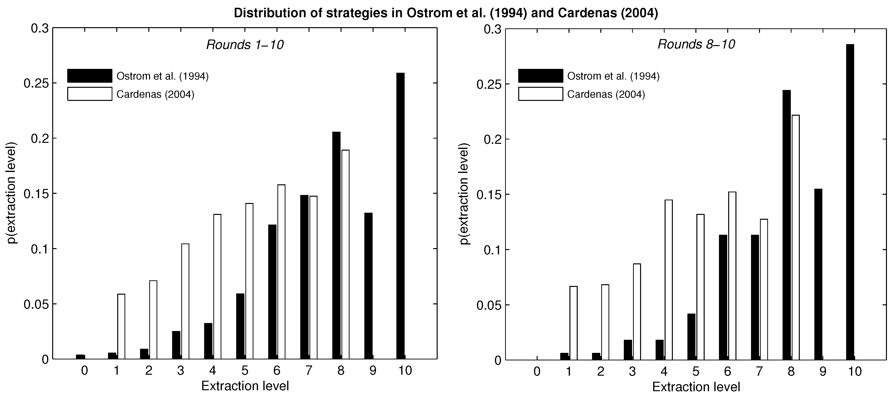
The left panel of Figure 1 displays the distribution of strategies aggregated by participants and rounds for the two experimental studies. In general, higher extraction levels are chosen with greater frequency. The maximum extraction is the modal choice in both settings, although it is the dominant action only in Cárdenas [11]. These aggregates mask considerable variation in action choice at the individual level across rounds: in Ostrom et al. [4], 73% of subjects chose the Nash equilibrium action at least once, while nobody chose this action in every round. In Cárdenas [11], 70% of subjects chose maximum extraction at least once, while less than 1% chose this action in every round.

The right panel of Figure 1 shows the distribution of actions for all participants in their last three rounds of play (Rounds 8–10). Higher extraction levels continue to be chosen with greater frequency than lower extraction levels on the whole, and there is a slight increase in the frequency of the modal choice.

Table 1 summarizes some of the key features of the two designs, including Nash equilibrium and joint surplus maximizing per-capita extraction levels. It also provides some descriptive statistics regarding the level and variability of extraction across rounds. The considerable variability across rounds in actions chosen by given individuals is revealed in Part (b) of the table.

Individuals sample, on average, between four and five different strategies. In Ostrom et al. [4], 7% of individuals limited themselves to a single action, and about 70% of them chose at least four distinct actions across the ten rounds. In Cárdenas [11], less than 1% of individuals sampled a single action, while 88% of them chose no less than four different actions. This suggests considerable experimentation on the part of subjects.

Figure 1. Distribution of strategies in Ostrom et al. (1994) and Cárdenas (2004).

Figure 1. Distribution of strategies in Ostrom et al. (1994) and Cárdenas (2004).

Table 1. Summary statistics for two experimental studies.

	Cárdenas [11]	Ostrom et al. [4]
a.Experimental setting
Number of subjects	230	56
Subjects per group	5	8
Number of rounds	10	10
Action set	{1,…,8}	{0,…,10}
Nash equilibrium	8	8
Surplus maximizing per-capita extraction	1	4.5
b. Strategies sampled in ten rounds
Median	6	4
Mean	5.37	4.16
Standard deviation	1.53	1.60
c. Average extraction levels
Rounds 1–5	5.16	7.56
Rounds 6–10	5.31	7.86
d. Within group standard deviation per round
Rounds 1–5	1.96	2.11
Rounds 6–10	1.94	1.93
Rounds 11–20 (subsample)	2.12	2.02

Table 1. Summary statistics for two experimental studies.

	Cárdenas [11]	Ostrom et al. [4]
a.Experimental setting
Number of subjects	230	56
Subjects per group	5	8
Number of rounds	10	10
Action set	{1,…,8}	{0,…,10}
Nash equilibrium	8	8
Surplus maximizing per-capita extraction	1	4.5
b. Strategies sampled in ten rounds
Median	6	4
Mean	5.37	4.16
Standard deviation	1.53	1.60
c. Average extraction levels
Rounds 1–5	5.16	7.56
Rounds 6–10	5.31	7.86
d. Within group standard deviation per round
Rounds 1–5	1.96	2.11
Rounds 6–10	1.94	1.93
Rounds 11–20 (subsample)	2.12	2.02

Next, consider the manner in which the average action choice varies over rounds, reported in Part (c) of Table 1. We see neither a convergence to the equilibrium action, nor to the efficient action in any of the experimental studies. In fact, the average extraction level remains quite steady at an intermediate level.

Part (d) of the table shows that the within-group variance does not seem to converge to zero or even to diminish systematically over time in either of the two studies. We observe that the average standard deviation per group per round oscillates around two and does not exhibit a trend across stages of the game. This stability in the variability of actions within groups is evidence against the hypothesis that individuals coordinate on a pure-strategy Nash equilibrium of a different game, obtained by transforming the material payoffs to allow for social preferences or reciprocity norms. For instance, if social preferences were to transform a social dilemma into a coordination game with multiple equilibria, convergence over time to one of these would result in the variance of within-group actions to decline over successive rounds.

To rule out the possibility that ten rounds are too few for convergence to be obtained, the last row of the table shows the average within-group standard deviation for the subsample of sessions in which interaction occurred over twenty rounds rather than ten. Again, we see that that the variance of actions is maintained at a roughly constant level throughout the additional ten rounds.

The distribution of actions chosen by participants and the stability over time of both the mean and the variance of this distribution suggest that conventional models based on social preferences cannot fully account for the data. In particular, the heterogeneity of actions at the level of an individual is suggestive of sampling and action selection in response to observed payoffs as in payoff sampling equilibrium or, alternatively, to the incorporation of noisy behavior into the best response function as in quantal response equilibrium.

We next show that both PSE and QRE can provide a good fit to the data. Both models predict the play of strictly dominated strategies in equilibrium, though for very different reasons. In QRE, dominated actions are played by mistake, while in PSE, they are played because they have a positive probability of being the most rewarding under the sampling procedure.

3. Payoff Sampling and Quantal Response

The key idea underlying the concept of payoff sampling equilibrium is that when faced with a novel strategic situation, individuals will experiment with actions, observe outcomes and choose among available choices based on realized payoffs. The problem of selecting an action is viewed, in effect, as a multi-armed bandit problem in which a given probability distribution over the actions of others determines the consequences of any given choice by the subject in question. A sampling equilibrium is a distribution that is self-generating, in the sense that the probability of selecting an action conditional on this distribution matches the probability with which this action is taken in the distribution.

Formally, consider a symmetric game with actions $\{a_1,...,a_m\}$, and let $p=(p_1,...,p_m)$ denote some arbitrary probability distribution over these actions. Now, suppose that a player samples each of the actions exactly once, and on each such trial, her opponent plays the mixed strategy given by p. Once all actions have been sampled, each will be associated with a realized payoff. Suppose that the player who is sampling selects the action with the highest realized payoff, breaking ties with uniform probability. Let $w_i\left(p\right)$ denote the probability that action $a_i$ is selected under this procedure. One interpretation of $w_i\left(p\right)$ is that it denotes the probability that action $a_i$ is selected when one’s opponent at each step of the sampling procedure is independently drawn from a large population in which a proportion $p_i$ always plays $a_i$.

A sampling equilibrium is simply a mixed strategy $p^{*}$ that satisfies:

$$w_i\left(p^{*}\right)=p_i^{*}$$

for all i. That is, for each action $a_i$, the likelihood that it will be selected is equal to the likelihood with which it is currently being played. This may be interpreted as a steady state of a dynamic process in which a large incumbent population is choosing actions in the proportions $p_1,...,p_n$, while new entrants choose actions in accordance with $w_1\left(p\right),...,w_n\left(p\right)$. Such a dynamic process is implicit in the justification for sampling equilibrium offered by Osborne and Rubinstein and requires that the rates of change ${\dot{p}}_i$ satisfy:

$${\dot{p}}_i>0\text{if}\text{and}\text{only}\text{if}{w}_i\left(p\right)>p_i$$

(3)

Stability with respect to this dynamic process can be used as a criterion for selection among multiple sampling equilibria.

The set of sampling equilibria can be large. It is easily seen, for instance, that every strict Nash equilibrium is also a sampling equilibrium. However, sampling equilibria can also have surprising features and involve the choice of actions that are strictly dominated. In fact, this can occur even in sampling equilibria that are stable under the dynamics (3).

In a symmetric n-player game with more than two players, a sufficient condition for the instability of a symmetric sampling equilibrium is that the corresponding action profile satisfies a condition called inferiority [8]. Specifically, a symmetric action profile $(a_q,\dots ,a_q)$ is said to be inferior if, when $n-2$ players continue to choose action $a_q$ while one player deviates to some action $a_i\ne a_q$, then for the remaining player, there exists at least one response $a_j\ne a_q$, such that, for this player, the resulting payoff is strictly preferred to the outcome at $(a_q,a_q,\dots ,a_q)$.

To see how a dominant strategy equilibrium profile can be inferior (and hence unstable under the sampling dynamics), consider a simple three-player, two-action public goods game in which each player has an indivisible unit endowment and can either keep it or contribute it to the provision of a public good. If the total contribution is $z\in \{0,1,2,3\}$, then a player contributing $y\in \{0,1\}$ to the public good obtains payoff $1-y+2z/3$. Clearly, a dominant strategy for each player is to contribute nothing, in which case the payoff to all players is one. However, this action profile is inferior: if one player contributes while another does not, the third player gets $4/3>1$ if she also contributes. Hence, the dominant strategy equilibrium is unstable under the dynamics (3) by Theorem 1 in [8], and strictly dominated strategies must be played with positive probability in any stable sampling equilibrium of the game 3.

It is easily verified that for the payoff function (2) and the parameter values chosen by Cárdenas [11], the dominant strategy equilibrium in which all players choose the maximum extraction level $x_i=8$ is inferior and therefore unstable. For this action profile, all five players receive a payoff of 320. If three of the five continue to choose the dominant strategy while one switches to any other extraction level, the remaining player can guarantee himself at least 337 by choosing an action other than the dominant strategy. Of course, the payoff from sticking to the dominant strategy would be still greater, but the inferiority condition is nevertheless satisfied. Hence, the dominant strategy equilibrium is unstable, and the only stable sampling equilibrium involves the playing of dominated strategies with positive frequency. The precise frequencies with which the various actions are chosen in the unique stable sampling equilibrium for this game, as well as that of Ostrom et al. [4] are described in more detail below.

Next, consider quantal response equilibrium. Here, the key idea is that subjects choose the strategy with the highest utility with a probability that depends on the utility difference with respect to alternative strategies [14]. It is assumed that the error rate (i.e., the chance of picking a suboptimal strategy) is common knowledge and is therefore accounted for by each subject in forming his best response. Consider again a symmetric game with actions $\{a_1,...,a_m\}$ with a probability distribution $p=(p_1,...,p_m)$ over actions. Letting $E_k\left(p\right)$ denote the expected payoff when playing action $a_k$ when faced with p, the logit QRE is given by the following set of $m-1$ equations:

$$p_k=\frac{e^{\lambda E_k\left(p\right)}}{{\sum }_{k=1}^K{e}^{\lambda E_k\left(p\right)}}$$

(4)

The parameter λ varies inversely with the error rate and may be interpreted as the degree of player rationality. When $\lambda \to \infty$ (the error rate tends to zero), subjects are unboundedly rational, and logit QRE is equivalent to Nash equilibrium. When $\lambda \to 0$ (the error rate is very large), subjects are acting randomly, and in equilibrium, each strategy is chosen with the same probability regardless of its expected payoff. A positive probability of play for dominated strategies is therefore guaranteed as long as we assumed a bounded degree of rationality captured through a finite value for λ.

For the experiments considered here, the predictions for the two-solution concepts (stable PSE and QRE) are shown in Table 2. The λ parameter for the QRE calculation corresponds to the value that minimizes the mean squared error for each CPRgame, i.e., the inverse of the error rate that best fits the distribution of optimal and suboptimal choices. The λ parameter was computed separately for each game using Equations (1) and (2). The optimal λ values are 0.09 and 18.2 for the reported data in Cárdenas [11] and Ostrom et al. [4], respectively 4.

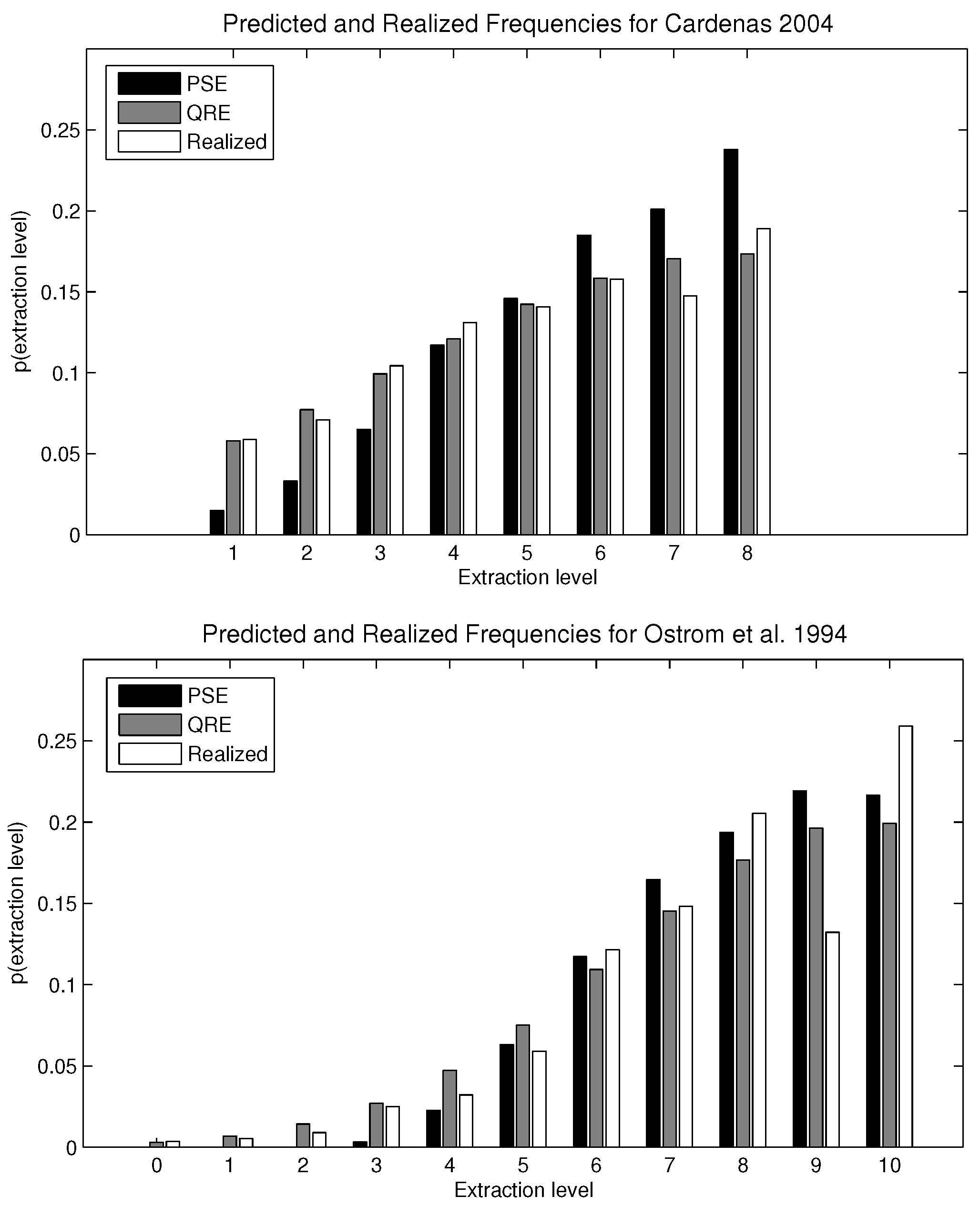
The comparison is also shown graphically in Figure 2. For Cárdenas [11], the mean squared errors for the QRE and the PSE models are 0.0001 and 0.0111, respectively. For Ostrom et al. [4], where the Nash equilibrium is interior, the mean squared errors are 0.0091 and 0.0105 for QRE and PSE, respectively. Allowing a different estimated parameter λ for each experimental setting, QRE outperforms PSE. The difference in their mean squared errors is especially stark in games where the Nash equilibrium is a corner solution, but the dominance of QRE over PSE is less clear if the individually-rational strategy is an interior point of the strategy set. Intuitively, the logistic QRE is very precise in the calibration of a straight line, as occurs in the Cárdenas [11] dataset, because the maximum extraction level allowed matches the Nash equilibrium. By definition, strategies closer to the optimal strategy are played with greater probability under QRE. Therefore, the predicted probabilities are strictly increasing. For the dataset from Ostrom et al. [4], QRE and PSE perform about equally well. The interior Nash equilibrium substantially lowers the predictive capacity of QRE.

Table 2. Computed equilibria for the CPRgames.

	Cárdenas [11]
	x = 0	x = 1	x = 2	x = 3	x = 4	x = 5	x = 6	x = 7	x = 8	x = 9	x = 10
Nash	-	0.000	0.000	0.000	0.000	0.000	0.000	0.000	1.000	-	-
PSE	-	0.015	0.033	0.065	0.117	0.146	0.185	0.201	0.238	-	-
QRE (λ = 0.09)	-	0.058	0.077	0.099	0.121	0.142	0.159	0.170	0.173	-	-
Observed	-	0.059	0.071	0.104	0.131	0.141	0.158	0.147	0.189	-	-
	Ostrom et al. [4]
	x = 0	x = 1	x = 2	x = 3	x = 4	x = 5	x = 6	x = 7	x = 8	x = 9	x = 10
Nash	0.000	0.000	0.000	0.000	0.000	0.000	0.000	0.000	1.000	0.000	0.000
PSE	0.000	0.000	0.00001	0.003	0.023	0.063	0.117	0.165	0.194	0.219	0.216
QRE (λ = 18.2)	0.003	0.007	0.014	0.027	0.047	0.075	0.109	0.145	0.177	0.196	0.199
Observed	0.004	0.005	0.009	0.025	0.032	0.059	0.121	0.148	0.205	0.132	0.259

Table 2. Computed equilibria for the CPRgames.

	Cárdenas [11]
	x = 0	x = 1	x = 2	x = 3	x = 4	x = 5	x = 6	x = 7	x = 8	x = 9	x = 10
Nash	-	0.000	0.000	0.000	0.000	0.000	0.000	0.000	1.000	-	-
PSE	-	0.015	0.033	0.065	0.117	0.146	0.185	0.201	0.238	-	-
QRE (λ = 0.09)	-	0.058	0.077	0.099	0.121	0.142	0.159	0.170	0.173	-	-
Observed	-	0.059	0.071	0.104	0.131	0.141	0.158	0.147	0.189	-	-
	Ostrom et al. [4]
	x = 0	x = 1	x = 2	x = 3	x = 4	x = 5	x = 6	x = 7	x = 8	x = 9	x = 10
Nash	0.000	0.000	0.000	0.000	0.000	0.000	0.000	0.000	1.000	0.000	0.000
PSE	0.000	0.000	0.00001	0.003	0.023	0.063	0.117	0.165	0.194	0.219	0.216
QRE (λ = 18.2)	0.003	0.007	0.014	0.027	0.047	0.075	0.109	0.145	0.177	0.196	0.199
Observed	0.004	0.005	0.009	0.025	0.032	0.059	0.121	0.148	0.205	0.132	0.259

Figure 2. Comparison between payoff sampling equilibrium (PSE), quantal response equilibrium (QRE) and experimental data.

Figure 2. Comparison between payoff sampling equilibrium (PSE), quantal response equilibrium (QRE) and experimental data.

Our claim is that the large difference in the implied value of λ is not due primarily to differences in the rationality of subjects or the complexity of the two games, but rather to the increasing difficulty of calibration when the action profile has an interior mode. The experimental pools are comparable, as both experiments were conducted with college students (although separated across time and space). The key difference between the games is the location of the socially-desirable and the individually-rational extraction levels within the choice set 5. It is striking, therefore, that the difference in implied values of λ reaches two orders of magnitude, as we move from 0.09–18.2, for games that are structurally similar and have a comparable number of players.

An alternative approach to calibration, as used in Selten and Chmura [16], is to define a unique value for λ that minimizes the joint mean squared errors. As is shown in the continuous bold line in Figure 3, this value of λ is 0.09, as in the Cárdenas [11] setting. The intuition behind this result is that QRE has a greater goodness of fit for the Cárdenas [11] sample for low values of λ, about one order of magnitude lower than the mean squared errors for Ostrom et al. [4], but it rapidly decreases its predictive success as λ increases. Using a single value for λ, the minimum mean squared error for QRE is 0.0784, much larger than the 0.0216 obtained for PSE. This difference is also observable in Figure 3 by comparing the black continuous curve with the gray straight line.

Figure 3. Aggregated mean squared errors as a function of λ.

Figure 3. Aggregated mean squared errors as a function of λ.

4. Statistical Tests

The visual correspondence between observed and predicted extraction levels is striking for the PSE and QRE models, but falls short of a statistical test of the model. We now turn to a more formal analysis of the match between theory and data.

Table 3 reports results from a regression of observed versus predicted frequencies of use for each action (both expressed as percentages). Of the m observations, one per available action, only $m-1$ are independently distributed. Therefore, we use a bootstrap procedure in which $m-1$ observations are randomly drawn in each one of the one hundred repetitions of the ordinary least squares estimation. Reported standard errors are corrected for the bootstrap procedure. Standard errors are larger than in the OLS regression with m observations, and the coefficients only differ after the third decimal number (regression results not shown but available upon request). Here, the prediction is a slope not different from unity, and lower slopes are indicative of a bias towards efficiency. We easily reject the hypothesis that the slopes equal zero for the two experiments under both equilibrium concepts. Furthermore, we cannot reject the hypothesis that the slope is one for the Cárdenas [11] data fitted with the QRE, but we clearly reject it for the PSE prediction.

For the Ostrom et al. [4] data, the relative goodness of fit is reversed. The slope coefficient for the PSE does not statistically differ from one, while for the QRE, we observe a slope considerably larger than unity along with a negative intercept. The reason for this poor calibration is that the low λ value that minimizes the mean squared error for the pooled data provides an exceptionally good fit for the game with the corner solution, at the cost of a very poor fit for the game with the interior solution.

Table 3. OLS: observed versus predicted percentage frequencies.

	Cárdenas [11]			Ostrom et al. [4]
	PSE	QRE		PSE	QRE	QRE
		$(\lambda =0.09)$			$(\lambda =0.09)$	$(\lambda =18.2)$
Slope (${\beta }_1$)	0.528 ***	0.982 ***		0.887 ***	44.06 ***	1.068 ***
	(0.0705)	(0.165)		(0.148)	(9.909)	(0.174)
Constant	5.901 ***	0.234		1.024*	−391.5 ***	−0.611
	(0.947)	(2.019)		(0.570)	(89.98)	(0.876)
Ho: ${\beta }_1$ = 1	101.76 ***	0.03		0.54	27.86 ***	0.15
	(0.0001)	(0.8737)		(0.4804)	(0.0005)	(0.7103)
Observations	8	8		11	11	11
R-squared	0.950	0.932		0.879	0.817	0.886

Robust standard errors in parentheses. *** $p<0.01$; ** $p<0.05$; * $p<0.1$.

Table 3. OLS: observed versus predicted percentage frequencies.

	Cárdenas [11]			Ostrom et al. [4]
	PSE	QRE		PSE	QRE	QRE
		$(\lambda =0.09)$			$(\lambda =0.09)$	$(\lambda =18.2)$
Slope (${\beta }_1$)	0.528 ***	0.982 ***		0.887 ***	44.06 ***	1.068 ***
	(0.0705)	(0.165)		(0.148)	(9.909)	(0.174)
Constant	5.901 ***	0.234		1.024*	−391.5 ***	−0.611
	(0.947)	(2.019)		(0.570)	(89.98)	(0.876)
Ho: ${\beta }_1$ = 1	101.76 ***	0.03		0.54	27.86 ***	0.15
	(0.0001)	(0.8737)		(0.4804)	(0.0005)	(0.7103)
Observations	8	8		11	11	11
R-squared	0.950	0.932		0.879	0.817	0.886

Robust standard errors in parentheses. *** $p<0.01$; ** $p<0.05$; * $p<0.1$.

To illustrate the dependence of the QRE goodness of fit on its parameter value, consider the regression estimates when the value of λ equals $18.2$, which minimizes the mean squared errors for the Ostrom et al. [4] data. As shown in the last column of Table 3, if this is the case, we cannot reject the hypothesis that the slope equals one.

We propose an additional test for the goodness of fit of PSE and QRE. We separately regress observed and predicted percentage frequencies on the extraction level using a quadratic specification to allow for nonlinearities. This allows us to compare the estimated coefficients for the observed data to the estimated coefficients for the predicted frequencies. The bootstrap procedure is also applied in this estimation by randomly drawing $m-1$ observations in each repetition. The results are shown in Table 4.

A Hausman test may be used to compare the regression coefficients, based on the null hypothesis that coefficients are the same across the two specifications. The Hausman statistic will be insignificant if the observed and predicted frequencies are sufficiently similar. We fail to reject the hypothesis of identical coefficients for the comparison between Cárdenas [11] data and predicted QRE, but we reject it for the PSE. For the Ostrom et al. [4] data, the roles are reversed yet again. We reject the hypothesis that the coefficients are structurally similar for the observed data and the QRE with $\lambda =0.09$, but we fail to reject it when comparing the observed data with the PSE. Nevertheless, if we set $\lambda =18.2$, we cannot reject the hypothesis that the polynomial calibration with the observed frequencies and the QRE are structurally the same.

Table 4. OLS: observed/predicted percentage versus the second order polynomial for extraction.

	Cárdenas [11]				Ostrom et al. [4]
	Observed	PSE	QRE		Observed	PSE	QRE	QRE
			$(\lambda =0.09)$				$(\lambda =0.09)$	$(\lambda =18.2)$
Extraction	2.776	3.643 **	2.957 ***		0.669	0.983	0.0731 ***	1.278
	(1.919)	(1.541)	(0.676)		(1.850)	(1.979)	(0.000)	(1.111)
Extraction${}^2$	−0.115	−0.0357	−0.134 *		0.179	0.170	−0.00189 ***	0.102
	(0.206)	(0.160)	(0.071)		(0.174)	(0.191)	(0.0000)	(0.107)
Constant	2.930	−2.982	2.598		−0.532	−1.789	8.791 ***	−0.864
	(4.420)	(3.487)	(1.619)		(4.471)	(4.914)	(0.0006)	(2.737)
Hausman test		47.91 ***	0.01			1.54	18.12 ***	0.45
		(0.0000)	(0.9949)			(0.4619)	(0.0001)	(0.7989)
Observations	8	8	8		11	11	11	11
R-squared	0.948	0.990	0.994		0.894	0.944	1.000	0.974

The reported ${\chi }^2$ statistic for each Hausman test corresponds to the structural comparison between observed; data and the relevant equilibrium prediction listed at the top of the column. Standard errors in parentheses. *** $p<0.01$; ** $p<0.05$; * $p<0.1$.

Table 4. OLS: observed/predicted percentage versus the second order polynomial for extraction.

	Cárdenas [11]				Ostrom et al. [4]
	Observed	PSE	QRE		Observed	PSE	QRE	QRE
			$(\lambda =0.09)$				$(\lambda =0.09)$	$(\lambda =18.2)$
Extraction	2.776	3.643 **	2.957 ***		0.669	0.983	0.0731 ***	1.278
	(1.919)	(1.541)	(0.676)		(1.850)	(1.979)	(0.000)	(1.111)
Extraction${}^2$	−0.115	−0.0357	−0.134 *		0.179	0.170	−0.00189 ***	0.102
	(0.206)	(0.160)	(0.071)		(0.174)	(0.191)	(0.0000)	(0.107)
Constant	2.930	−2.982	2.598		−0.532	−1.789	8.791 ***	−0.864
	(4.420)	(3.487)	(1.619)		(4.471)	(4.914)	(0.0006)	(2.737)
Hausman test		47.91 ***	0.01			1.54	18.12 ***	0.45
		(0.0000)	(0.9949)			(0.4619)	(0.0001)	(0.7989)
Observations	8	8	8		11	11	11	11
R-squared	0.948	0.990	0.994		0.894	0.944	1.000	0.974

The reported ${\chi }^2$ statistic for each Hausman test corresponds to the structural comparison between observed; data and the relevant equilibrium prediction listed at the top of the column. Standard errors in parentheses. *** $p<0.01$; ** $p<0.05$; * $p<0.1$.

To summarize, the statistical tests confirm what visual inspection led us to believe: the concepts of stable sampling equilibrium and quantal response equilibrium can explain a great deal of the variation in frequencies from the experimental data. We also observe that QRE fits better than PSE for the game with a corner Nash equilibrium, while the opposite is true when the individually-rational strategy is an interior point in the strategy set.

After exploring how PSE and QRE fit the experimental data separately, our next step is to compare the relative predictive success of the two models. Following the comparison made in Selten and Chmura [16], we apply the Wilcoxon-matched pairs signed rank test to the mean squared errors of the two equilibrium models. For the computation in the QRE, we use $\lambda =0.09$, a value that minimizes the mean squared errors of the whole sample, i.e., the two experimental settings. We consider each group as an independent observation, having a total of 46 observations for the data in Cárdenas [11] and seven observations for the data in Ostrom et al. [4].

Results of the statistical tests are displayed in Table 5. We do not find any differences in the predictive success for the whole sample. Nevertheless, if we performed the Wilcoxon signed rank test separately for the two experimental settings, the results are different. Moreover, they confirm what we have been discussing in this section: for the game with the extreme Nash equilibrium, from Cárdenas [11], QRE has greater predictive power than PSE, and the test is significant at the five percent level. For the game with the internal Nash equilibrium, Ostrom et al. [4], the larger predictive power of PSE is confirmed by this test. The statistical significance at the five percent level is particularly surprising given the limited number of available observations.

Table 5. Wilcoxon signed rank test.

	Experimental Datasets
	Pooled	Cárdenas [11]	Ostrom et al. [4]
Independent groups	53	46	7
z	0.580	2.540 **	−2.366 **
p-value	0.562	0.011	0.018

$z>0$ indicates a better fit from QRE. $z<0$ indicates a better fit from PSE. *** $p<0.01$; ** $p<0.05$; * $p<0.1$.

Table 5. Wilcoxon signed rank test.

	Experimental Datasets
	Pooled	Cárdenas [11]	Ostrom et al. [4]
Independent groups	53	46	7
z	0.580	2.540 **	−2.366 **
p-value	0.562	0.011	0.018

$z>0$ indicates a better fit from QRE. $z<0$ indicates a better fit from PSE. *** $p<0.01$; ** $p<0.05$; * $p<0.1$.

5. Alternative Models

We have focused to this point on two alternatives to Nash equilibrium: payoff sampling and quantal response. There are, of course, other models of behavior in experimental games. These can be divided into two groups: those that look for departures from Nash equilibrium based on learning or reasoning and those that maintain the Nash hypothesis, but allow for the possibility that material payoffs do not define the game that individuals are actually playing, for instance because of social preferences or reciprocity norms. Both of these approaches have given rise to substantial literature in their own right, as well as the recent development of hybrid models.

In an analysis of data from multiple $2\times 2$ games, Selten and Chmura [16] consider four alternatives to Nash equilibrium 6. In addition to the two discussed extensively above, they consider action sampling equilibrium (ASE) and impulse balance equilibrium (IBE). Under action sampling, individuals take a random sample of observations of their opponent’s strategies and then optimize against this sample. Under impulse balance, it is assumed that, being informed of his realized and foregone payoffs, the subject could experience downward or upward impulses after comparing the realized payoff with his “natural aspiration level”. Under this equilibrium concept, impulses towards one strategy must be equally compensated by impulses towards the other strategy. Chmura et al. [18] extend their comparison between impulse balance equilibrium and Nash equilibrium to $3\times 3$ games with completely mixed and partially mixed equilibria and find that generalized impulse balance performs best in predicting the experimental data.

When these concepts are generalized to allow for multiple players and actions and applied to the common pool resource game, action sampling simply reduces to the dominant strategy equilibrium, while impulse balance is not well defined. The impulse balance equilibrium can be computed if strategies are dominated by a mixture of two pure strategies, as in Chmura et al. [18], but not when they are dominated by a pure strategy, as in our CPR games. For games with dominant strategies, impulse balance equilibrium cannot be calculated, because, by construction, all of the downward impulses are zero for the dominant strategy.

To see why action sampling reduces to the dominant strategy equilibrium, recall that a player takes a random sample of m observations of his counterpart’s strategies and applies a best response to this sample. Since the effect of effort levels is additive in common pool resource games, the only payoff relevant attribute of the sample is the aggregate extraction $X_{-i}={\sum }_{j\ne i}{x}_j$ of other players, and the best response to any given sample is therefore always the dominant strategy.

An alternative behavioral model in which dominated strategies might be played with positive probability is level-k reasoning [19,20]. This model assumes a heterogeneous population in terms of their degree of iterative reasoning k. Choices from Level-0 players are assumed to be randomly chosen, i.e., they are drawn from the strategy set with the same probability. Level-1 players best respond to Level-0, Level-2 to Level-1, and so on. Let us define α as the fraction of Level-0 subjects and $1-\alpha$ as the fraction of all level-k subjects with $k\ge 1$. In a game with J pure strategies, the predicted proportion of play will be $\alpha /J$ for all dominated strategies and $1-\alpha (1-J)/J$ for the dominant strategy. This model fails to predict that less costly strategies are played more often even if they are strictly dominated, as is shown in Figure 1.

A different strand of the literature on models of behavior in experimental games develops the idea that the material payoffs faced by experimental subjects do not accurately reflect their objective functions, because they care about the entire payoff distribution and, perhaps, also because their utilities are belief dependent, as in the theory of psychological games 7. While the persistent variability in actions across rounds in Table 1 is evidence against coordination on a pure-strategy Nash equilibrium of a transformed game, it is nevertheless likely that social preferences and norms do play a significant role in accounting for the choices of subjects. This is especially the case for results from field experiments. In addition to the experiment with student populations, Cárdenas [11] also conducted a number of trials with villagers for whom common pool resource management is a routine activity. These subjects were less likely to choose the dominant strategy (15%, rather than 19% of the time) and more likely to choose efficient extraction (12% of the time, more than twice as often as the students). One-third of villagers never chose the dominant strategy in any round.

For this population of villagers, the mean squared errors for the QRE (with $\lambda =0.09$) and PSE models are 0.0145 and 0.0473, respectively. These values are considerably larger than those derived from the student sample, for which mean squared errors were 0.0001 and 0.0111, respectively. The error for the sample of villagers drops to 0.0011 for the QRE model if the λ parameter is recalibrated to 0.000. The increase in predictive power for QRE here comes at the cost of assuming a very large error rate or, equivalently, null rationality among the villagers. A more plausible interpretation is that social preferences or norms of restraint play a greater role among villagers than they do among the pool of urban students, mitigating the effects of sampling dynamics. Put differently, any explanation of behavior based on sampling needs to take into account the fact that subjects have other-regarding preferences and that these may differ systematically across different populations.

These two distinct approaches (social preferences and learning) have been merged in recent work by Arifovic and Ledyard [12], who embed social preferences in a learning model with the goal of accounting for the basic stylized facts emerging from public goods experiments. Social preferences are introduced by allowing for individuals to care about both efficiency and envy, where the former is represented by average payoffs and the latter by any shortfall in one’s own payoff relative to the average. Learning is modeled as follows. At each period, there is a finite list of remembered actions from which choices are made in accordance with a probability measure. The items on this list need not be unique: a given action can have multiple replicates. Replication in each period takes place on the basis of hypothetical performance in the immediately preceding period, with an action that would have performed poorly being replaced by one that would have done better. This measure of hypothetical performance also determines which action is played in any given period, with higher valued actions being selected with greater likelihood. In addition, the list of remembered actions itself changes over time, as incumbent items are replaced by novel ones with some probability.

The Arifovic and Ledyard model has six free parameters, while sampling equilibrium has none. This makes a meaningful performance comparison between the two approaches difficult, and we have accordingly focused on the more parsimonious quantal response model instead. Here, we find sampling to be very competitive, especially if the free parameter for quantal response is constrained to be the same across experiments with a similar payoff structure and degree of complexity. More generally, the development of comprehensive models with many free parameters incorporating a variety of psychological effects alongside the exploration of simple, parsimonious models with few if any free parameters seems to be worthwhile.

6. Conclusions

Observed behavior in laboratory experiments under a common-pool resource dilemma shows that individuals often choose strictly dominated strategies even after a number of repeated rounds. This behavior yields outcomes that deviate systematically from the Nash equilibrium and allow these groups to mitigate the tragedy of the commons.

We have argued in this paper that a simple model of behavior based on the dynamics of sampling can be used to account for these experimental regularities. Even without incorporating other-regarding preferences, qualitative predictions based on stable sampling equilibrium match observed patterns remarkably well. In particular, the predicted lower frequencies for strategies that are more individually costly appear as a consistent and striking feature of the data when one restricts attention to the typical laboratory subject pools.

A distinctive feature of the sampling equilibrium concept is that it is parameter-free. The one-parameter family of quantal response equilibria can outperform sampling equilibrium in individual treatments, especially those involving corner solutions. However, when the error-rate parameter is constrained to be the same across treatments and games with interior solutions are also considered, then sampling equilibrium provides a somewhat superior fit.

We do not claim that the concept of stable sampling equilibrium alone can account for the experimental findings; it is clear that social preferences and norms also play a role, especially for populations with a high dependence on common property, close proximity and enduring social ties. Our purpose, rather, has been to bring the attention of experimental researchers to a versatile theoretical construct that might be very effective in accounting for observed data when used in conjunction with other approaches.

We suspect that the effectiveness of the sampling equilibrium concept in the common pool resource environment arises from the complexity of the game: there are multiple players; many actions for each of them; and the mapping from action profiles to payoffs is far from transparent. Under these conditions, it makes sense to explore options and to settle on those that happen to produce favorable results.

Merging a theory of social preferences with sampling dynamics seems both tractable and worthwhile, although the resulting model will clearly not be parameter-free. Furthermore, the concept of stable sampling dynamics is versatile and can be applied to any normal form game. Testing predictions based on this hypothesis in other settings is accordingly an interesting and potentially fruitful area for future research.