A Loser Can Be a Winner: Comparison of Two Instance-based Learning Models in a Market Entry Competition

Abstract

This paper presents a case of parsimony and generalization in model comparisons. We submitted two versions of the same cognitive model to the Market Entry Competition (MEC), which involved four-person and two-alternative (enter or stay out) games. Our model was designed according to the Instance-Based Learning Theory (IBLT). The two versions of the model assumed the same cognitive principles of decision making and learning in the MEC. The only difference between the two models was the assumption of homogeneity among the four participants: one model assumed homogeneous participants (IBL-same) while the other model assumed heterogeneous participants (IBL-different). The IBL-same model involved three free parameters in total while the IBL-different involved 12 free parameters, i.e., three free parameters for each of the four participants. The IBL-different model outperformed the IBL-same model in the competition, but after exposing the models to a more challenging generalization test (the Technion Prediction Tournament), the IBL-same model outperformed the IBL-different model. Thus, a loser can be a winner depending on the generalization conditions used to compare models. We describe the models and the process by which we reach these conclusions.

1. Introduction

A choice prediction competition was organized by Erev, Ert, and Roth [1]. This modeling competition focused on decisions from experience in market entry games (hereafter, market entry competition, MEC, http://sites.google.com/site/gpredcomp/). The market entry games involved four interacting players who had to decide between entering a market (a risky alternative) and staying out of the market (a safe alternative) in a number of trials. The payoffs of entering the market decreased with the number of entrants, and were also subject to probabilistic influences on the outcomes. Human data from an estimation set was made available for researchers, who used it to calibrate their models. These models were then submitted to compete over the best predictive value in a new dataset called the competition set.

Our team (the co-authors of this paper) submitted two versions of the same cognitive model to the competition. The cognitive model submitted was developed according to the Instance-Based Learning Theory (IBLT [2]). One version of the IBL model assumed that the four players in the game had identical characteristics. As it will be explained later, this model, called IBL-same, included the same set of parameter values for each of the four players in the game. The other version of the IBL model, called IBL-different, assumed heterogeneity of the four players in the game, and included different sets of parameter values for each of the four players in the game. The IBL-different model won the runner-up prize of the competition among 25 other submissions, while IBL-same model achieved the 11th place.

The current paper reports the process and main lessons learned through the submission of the two versions of the same IBL model. First, we describe the MEC and behavioral methods used in the estimation and competition sets. Next, we summarize IBLT and describe the IBL model developed for the MEC. Next, we discuss the process by which the model parameters were determined in both the IBL-same and IBL-different models. We discuss the calibration (or fit) of each model to the estimation set, and present our a-priori expectations of the performance of the two models in the competition set of the MEC. Then, we discuss the actual performance of the two models in the competition set. We follow with discussing the unexpected results of the MEC, and show that the IBL-same (the loser) model outperforms the IBL-different (the winner) model under more challenging generalization conditions in a different dataset. To conclude, we discuss the main lessons learned from our participation in the MEC.

2. Market Entry Competition and Behavioral Methods

Each game in the MEC consists of four players who make individual choices in a number of trials. In each trial of a game, each of the four players decides individually between entering a risky market (risky alternative) or staying out (safe alternative). The payoff for player i if entering the market at trial t is

$$10-k(E)+G_t$$

Where k is a parameter drawn (with equal probability) and with replacement from the set {2, 3, 4, 5, 6, 7}.

E is the number of entrants in trial t, and G_t is a binary gamble that yields “H with probability Ph; and L otherwise.” H is a positive number and L is a negative number, determined according to the algorithm described in Appendix 1 of Erev et al. [1].

The payoff for a player i if staying out in trial t is

$$\text{round}\left(G_t/S\right)\text{with}\text{p}=0.5;\text{and}-\text{round}\left(G_t/S\right)\text{otherwise}$$

Where S is a parameter drawn (with equal probability) and with replacement from the set {2, 3, 4, 5, 6}.

Thus, the payoff for a player depends on the player's own choice (to enter or stay out), the choices of the other players (E, such that the more people enter the market the lower the payoff from entry), and the trial's outcome of a gamble (G_t).

There were a total of 40 games used in the estimation set. These games were determined by a random selection of the parameters: k, S, H, Ph, and L (using the algorithm described in Appendix 1 in Erev et al. [1]). One hundred and twenty students participated in the estimation set. The set involved 8 sessions, each of which included between 12 and 20 participants. Each session used 10 of the 40 games, so that each subset of 10 games was run twice in a counterbalanced order. In each session, each participant was randomly matched with three other participants, and each of the 10 games was played for 50 trials. Participants did not receive a description of the payoff calculation, but they obtained feedback after each trial. Feedback included the payoff from their own choice and their “forgone” payoff (i.e., the payoff they would have obtained had they selected the other alternative).

Results were grouped for each game and the 50 trials played in each game were separated into a first and a second block of 25 trials each. The dependent measures of performance used in Erev et al. [1] are the average of the following for each of the two blocks:

• Entry rate: the proportion of entry decisions

• Efficiency: the mean observed payoffs

• Alternation rate: the proportion of times players changed their choices (from entering to staying out or from staying out to entering) between trials

Thus, six statistics were used as dependent measures.

2.1. Competition Criteria and Dataset

The human data for the estimation set was made available to researchers ahead of time. They were allowed to analyze the data, study the observed behavior, and build their own models. After the submission deadline, the competition set was run using the same behavioral procedures used in the estimation set. The competition set involved the selection of 40 games different from those used in the estimation set, but the games were also determined by the same selection algorithm (Appendix 1 in [1]). The MEC focused on the models' predictions of the six statistics described above in the new 40 competition set problems. Currently, both the estimation and competition studies are publicly available, posted by the organizers in the MEC web page ( http://sites.google.com/site/gpredcomp/study-results/competition-study).

Twenty-five models were submitted to the competition and each of the models was evaluated using the mean squared deviation (described in detail in Erev et al. [1]) between the models' predictions and the observed performance in the competition set. Each model obtained a final score, the nMSD (normalized mean squared deviation). The nMSD is the mean of the six normalized mean squared deviations (MSD) for each of the six statistics described above. Each of the MSDs for each of the dependent measures was calculated in the following three steps: (1) compute the squared deviation between the model's prediction and the observed statistic in each of the 40 games; (2) compute the mean squared deviation over all the 40 games; and (3) normalize each score by the variable's estimated error variance. The model with the lowest nMSD score won the MEC.

3. An Instance-Based Learning Model

The cognitive model submitted to the MEC is based on a cognitive theory of decisions from experience, Instance-Based Learning Theory (IBLT), originally developed to explain and predict learning and decision making in dynamic decision-making environments [2].

IBLT proposes a key representation of cognitive information: an instance. An instance is a representation of each decision alternative, often consisting of three parts: a situation (a set of attributes that define the alternative), a decision, and an outcome resulting from making that decision in that situation. The theory also proposes a generic decision-making process that starts by recognizing and generating instances through interaction with an environment, and finishes with the reinforcement of the instances that led to good decision outcomes through feedback from the environment. The general decision-making process is explained in detail in Gonzalez et al. [2], and it involves the following steps: The recognition of a situation from an environment (a task) and the creation of decision alternatives; the retrieval of similar experiences from the past to make decisions, or the use of decision heuristics in the absence of similar experiences; the selection of the best alternative; and, the process of reinforcing positive experiences through feedback.

At each decision stage, IBLT selects an instance that has the highest utility (blended value, explained below). The different parts of an instance and the selection of an alternative are built through the general IBLT decision process: creating a situation from attributes in the task, creating an expected utility for making a decision, and updating the utility value according to the outcomes observed from an alternative. Instances corresponding to outcomes accumulate over time and their blended values depend on the availability of those instances in memory. This availability is measured by a statistical mechanism called Activation, originally developed in the ACT-R cognitive architecture [3].

3.1. The IBL Model for the MEC

IBL models are particular representations of IBLT for specific tasks. Many IBL models have been developed in a wide variety of tasks, including dynamically-complex tasks [2-5], training paradigms of simple and complex tasks [6,7], simple stimulus-response practice and skill acquisition tasks [8], repeated binary-choice tasks [9,10] among others. Although most of the IBL models developed are task specific, a recent IBL model showed that it generalizes well to multiple repeated-choice tasks that share the same task structure. The IBL model reported in Lejarraga, Dutt, and Gonzalez was built to predict performance in individual binary-choice tasks, and generalized accurately to choices in a repeated-choice task, probability-learning tasks, and repeated-choice tasks with changing probability of outcomes as a function of trials [10]. The IBL model for the market entry task is an extension of the model reported in Lejarraga et al. [10].

Instances in the repeated choice and MEC model are much simpler than in other IBL models, as the structure of these tasks is simple. Each instance consists of a label that identifies an alternative in the task and the outcome obtained (i.e., a button label and its observed outcome). For example (Enter, $4), is an instance in which the decision was to enter the market and the outcome as a result of that choice was $4. In the MEC, since participants also observed forgone payoffs, another similar instance was created for the obtained foregone payoff in each decision made, for example (Stay Out, $3).

In each trial t of a market-entry game, the process of selecting alternatives in the model starts with an inertia rule (Equation 1 below), which determines whether the previous choice in the task is repeated according to the surprise-triggers-change hypothesis by Nevo and Erev [12]. If the previous choice is not repeated, then the alternative with the highest blended value is selected (Equation 5 below). The blended value of an alternative is calculated in each trial t of the game and it is a transient value that depends on the outcome stored in an instance and the probability of retrieval of that instance from memory (Equation 6 below). Furthermore, the probability of retrieval of an instance from memory is a function of its activation in memory (activation is a function of the recency, frequency and noise in the retrieval of an instance) (Equation 7 below).

3.2. Inertia Mechanism

Erev et al. [1] report several behavioral regularities found in the estimation set in the MEC: Surprise-triggers-change from choosing one alternative to the other, and the presence of strong inertia in repeated choice. These two effects relate to sequential dependencies between choices in human data, measured with the Alternation rate. These sequential dependencies in choices over time have also been demonstrated by Biele, Erev, and Ert [11] and Nevo and Erev [12].

Our model in Lejarraga et al. [10] was not built to account for alternations, but rather to account for the proportion of risky choices in repeated-choice tasks. Given that many influential models of repeated choice have found a weak relationship between the generic measures of performance and sequential dependencies [13,14], we investigated how IBL models are able to account for sequential dependencies and the tradeoffs between the proportion of risky choices and the proportion of alternations in repeated-choice tasks [15]. To capture sequential dependencies in the MEC data, we built on the surprise-triggers-change hypothesis by Nevo and Erev [12] and proposed a new inertia mechanism that considers blended values instead of running averages. This mechanism is determined at the moment of making a choice in trial t+1 by a simple rule:

If the draw of a random value in the uniform distribution

$$U\left(0,1\right)<{\left(\mathit{\text{pInertia}}\right)}^{\text{Surprise}\left(\text{t}\right)}$$

(1)

Then

Repeat the choice as in the previous trial

Else

Select the alternative with the highest blended value as per Equation 2 (below)

The pInertia or the Probability of Inertia is a free parameter between 0 and 1 and initially defined at 0.30, according to Biele et al. [11]. The value of the Surprise(t) is assumed to depend on the gap (absolute difference) between an expectation of the outcome and the outcome actually received. In our inertia mechanism this is the absolute difference between the observed outcome and the blended value for that alternative. Since forgone payoffs are observed in the market entry games, the gap is calculated for the two alternatives, enter and stay out, as follows:

$$\text{Gap}\left(\text{t}\right)=½\times (|{\text{outcome}}_{\text{Enter}}\left(\text{t}-1\right)-{\text{V}}_{\text{Enter}}\left(\text{t}-1\right)|+|{\text{outcome}}_{\text{Stay out}}\left(\text{t}-1\right)-{\text{V}}_{\text{Stay out}}\left(\text{t}-1\right)|)$$

(2)

The outcome _Enter (t–1) is the observed or foregone outcome obtained upon entering the market in the last trial and outcome _{Stay out} (t–1) is the observed or foregone outcome obtained upon staying out. The V _Enter (t–1) and V _{Stay out} (t–1) are the blended values of the two alternatives obtained in the last trial (the calculation of blended values is defined below).

The surprise in trial t is normalized by the mean gap (in the first t−1 trials):

$$\text{Surprise}\left(\text{t}\right)=\text{Gap}\left(\text{t}\right)/\left[\text{Mean}\left(\text{Gap}\left(\text{t}\right)\right)+\text{Gap}\left(\text{t}\right)\right]$$

(3)

The Mean(Gap(t)) is defined over 50 trials of a market entry game as:

$$\text{Mean}\left(\text{Gap}\left(\text{t}\right)\right)=\text{Mean}\left(\text{Gap}\left(\text{t}-1\right)\right)\left(1-1/50\right)+\text{Gap}\left(\text{t}\right)\left(1/50\right)$$

(4)

Erev et al. [1] justified the gap-based formulation of surprise by the observation that the activity of certain dopamine-related neurons is correlated with the difference between average past payoff (or the blended value) and the present outcome. This assumption is the only extension to the model reported in Lejarraga et al. [10] needed to account for the sequential dependencies reflected in the proportion of alternations in the market entry games. Naturally, the higher the value of pInertia, the more the IBL model will repeat its choice.

3.3. The General IBLT Mechanisms

In making a choice, IBLT selects the alternative with the highest blended value, V [16] resulting from all instances belonging to an alternative. The blended value of alternative j is defined as

$$V_j={\sum }_{i=1}^n{p}_i{x}_i$$

(5)

Where x_i is the value of the observed (obtained or foregone) outcome in the outcome slot of an instance i corresponding to the alternative j, and p_i is the probability of that instance's retrieval from memory (for the MEC as noted in Equation 2, the value of j is either to enter or to stay out). The blended value of an alternative (its utility) is the sum of all observed outcomes x_i in the outcome slot of corresponding instances in memory, weighted by their probability of retrieval. In any trial t, the probability of retrieval of instance i from memory is a function of that instance's activation relative to the activation of all other instances corresponding to that alternative, given by

$$P_{i,t}=\frac{e^{A_{i,t/\tau }}}{{\sum }_j{e}^{A_{j,t/\tau }}}$$

(6)

Where τ is random noise defined as $=\sigma \times \sqrt{2}$, and σ is a free noise parameter (more details below). Noise in equation 2 captures the imprecision of recalling instances from memory.

The activation of each instance in memory depends upon the Activation mechanism originally proposed in the ACT-R architecture [3]. A simplified version of the activation mechanism that relied on recency and frequency of use of instances in memory was sufficient to capture human choice behavior in several repeated-choice and probability-learning tasks [10]. For each trial t, Activation A_i,t of instance i is:

$$A_{i,t}=\mathit{\text{ln}}\left({\sum }_{t_i\in \left\{1,\dots ,t-1\right\}}{\left(t-t_i\right)}^{-d}\right)+\sigma .\mathit{\text{ln}}\left(\frac{1-{\gamma }_{i,t}}{{\gamma }_{i,t}}\right)$$

(7)

Where d is a free decay parameter, and t_i is the time period of a previous trial where the instance i was created or its activation was reinforced due to an outcome in the task corresponding to the instance in memory. The summation will include a number of terms that coincides with the number of times that an outcome has been observed in previous trials and that the corresponding instance i's activation has been reinforced in memory. Therefore, the activation of an instance corresponding to an observed outcome increases with the frequency of observation (i.e., by increasing the number of terms in the summation) and with the recency of those observations (i.e., by small differences in t - t_i of outcomes that correspond to that instance in memory). The decay parameter d affects the activation of the instance directly, as it captures the rate of forgetting. In ACT-R, the d parameter is almost always set to 0.5. The higher the value of the d parameter, the faster the decay of memory, and the harder it is for the model to recall distant memories of its instances with outcomes.

The γ_i,t term is a random draw from a uniform distribution bounded between 0 and 1, and the $\sigma .\mathit{\text{ln}}\left(\frac{1-{\gamma }_{i,t}}{{\gamma }_{i,t}}\right)$ term represents Gaussian noise important for capturing variability of human behavior. The σ is a free noise parameter that has no default value in ACT-R, but that it has been found to have a mean of 0.45 in many ACT-R studies [17]. Higher σ values imply greater noise in the retrieval of instances from memory.

3.4. Special Treatment of the First Trial

In the first trial of a game, the model has no past instances in its memory from which to calculate blended values. Therefore, the model makes a selection between two instances in memory for the first trial by assuming some initial blended values. Each initial blended value corresponds to one of the two alternatives, entering or staying out. The blended value of the pre-populated instances may represent the expectations that participants bring to the laboratory [10]. The choice of the blended values in the two instances was motivated from the observed entry rate in the first trial of the estimation set. We found that the observed entry rate was about 73% (>50%) in the first trial of the estimation set, i.e., more than 50% of the participants entered the market in the first trial. We speculate that one reason for the higher entry rate could be that the experiment was framed as a market entry competition. Due to this observation and the fact that the ratio of the blended values assigned to the two instances determines the entry rate in the first trial in the model, we assigned a +94 value as the blended value of the instance corresponding to the enter alternative and a +34 value to the blended value of the instance corresponding to the stay out alternative. As seen, the ratio of the value assigned to the instance corresponding to the “enter” alternative to the sum of the values assigned to both instances, i.e., 94/(94 + 43) computes to 73%, i.e., the observed entry rate in the first trial in the estimation set. In the first trial, a decision to enter or stay out is also based solely upon these blended values for each pre-populated instance. The inertia mechanism is used from the second trial onwards. As the value of V _Enter (0) and V _{Stay out} (0) do not exist, Gap (1) is calculated by replacing V _Enter (0) and V _{Stay out} (0) by 94 and 34 in Equation 2. Also, the Mean(Gap(1)) is taken to be a very small number close to 0 (= .00001). Our assumption on Mean(Gap(1)) is similar to that by Erev et al. [1].

4. Two Versions of the IBL Model: IBL-same and IBL-different in the Estimation Set

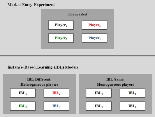
As described above, the IBL model for the MEC consists of three free parameters that define a decision maker: d, σ, and pInertia. We created two different submissions for the MEC: the IBL-same and IBL-different. Each of the two submissions included four identical copies of the same IBL model, where each copy represented one of the four simulated players in a market-entry game. Furthermore, each copy (or simulated player) had three free parameters: d, σ, and pInertia.

The only difference between the IBL-same and the IBL-different submissions is that the IBL-different model used a different set of model parameters for each of the four copies (or simulated players) of the IBL model. In contrast, the IBL-same used the same values of the three parameters in each of the four copies. Thus, the IBL-different allowed for 4 different values of d, 4 different values of σ, and 4 different values of pInertia. The IBL-same, in contrast, assumed the same d, σ, and pInertia values for all the four simulated participants in the model. The values of the parameters for both submissions were determined through an optimization process to fit the observed data in the estimation set.

4.1. Optimization of Parameters through a Genetic Algorithm

The parameter values of the IBL-different and IBL-same models were obtained through an optimization process that maximized the fit of the model's data to human behavior in the estimation set. The process involved an optimization of the parameter values for each model involving a genetic algorithm. The goal of the generic algorithm was to find the set of parameters that minimized the error between the model's predictions and the observed behavior. Specifically, the genetic algorithm attempted to minimize the normalized mean squared deviation (nMSD).

The genetic algorithm tests different combinations of parameters in a model to minimize the nMSD between predictions and observed behavior across the 40 problems in the estimation set of the MEC. First, different parameter combinations (N) are selected and tested. This first group of parameters combinations is the referred to as the first “generation.” Each test of a combination of parameters involves running the model multiple times (i.e., multiple simulated participants) and obtaining the mean prediction, which is then compared to the mean behavior across the six measures that determine the nMSD. The parameter combinations are then ranked from best fitting to worst fitting based upon the calculated nMSD values. After ranking, the best half of the parameter combinations are kept (N/2), and the rest (N/2) are discarded. The parameter combinations that are kept are then duplicated, bringing the number of parameter combinations back to the original amount (N). Then, the N parameter combinations are paired off with each other at random (thus forming N/2 pairs). Now, each parameter combination exchanges some of its adjustable parameter values with the corresponding parameter value of its partner (this is called “reproduction”). For example, suppose the following two three-parameter combinations have been paired off: (a1, b1, c1) and (a2, b2, c2). Then, due to the exchange of the adjustable parameter values a1 and a2 in the pair, the resulting parameter combinations will be (a2, b1, c1) and (a1, b2, c2). The exchange of parameters defines a new generation that is different from the previous generation but maintains characteristics (i.e., the parameter values) of the previous generation's best cases. After the exchange, a new set of N parameter combinations is tested in the model and new nMSDs are obtained. The process is repeated for 10,000 generations. This value is extremely large and thus ensures a very high level of confidence in the optimized parameter values obtained. We simulated 100 four-participant teams for each combination of parameters in the model during optimization to derive an nMSD. Once the optimization was completed we increased the number of four participant teams in the model from 100 to 1,000. This value ensures that a model's prediction for the dependent measures is stable and does not change much from generation-to-generation for the same parameter combination used in the model.

For the purpose of optimizing the two IBL models using the genetic algorithm, the d and σ parameters were varied between 0.0 and 10.0, and the pInertia parameter was varied between 0.0 and 1.0. The assumed range of variation of d and σ parameters in the models is large and ensures that the optimization does not miss the minimum nMSD value on account of a small range of parameter variation.

The fitted values of the three parameters for the IBL-same model were:

d = 1.97, σ = 1.17, and pInertia = 0.23

The fitted values of the three parameters for the four simulated participants in the IBL-different submission were:

Player 1: d = 3.00, σ = 1.08, and pInertia = 0.13

Player 2: d = 1.73, σ = 1.44, and pInertia = 0.63

Player 3: d = 1.22, σ = 1.16, and pInertia = 0.02

Player 4: d = 2.93, σ = 1.26, and pInertia = 0.22

Because a larger number of free parameters allows models greater flexibility, the IBL-different model fitted the human data on the estimation set slightly better (nMSD = 1.153) than the IBL-same model (nMSD = 1.308).

These predictions of the IBL models were obtained for their best fitting parameters (determined above) for a set of 1,000 simulated four-player teams. The choices of all participants were averaged to obtain the six dependent measures used to evaluate the competing models: Entry rate, Efficiency, and Alternation rate in the first block (B1, the first 25 trials) and the second block (B2, last 25 trials) of each game. The MSDs and the nMSD value of each model were obtained by the three-step procedure detailed above.

Table 1. Summary of fit results in the Estimation set.

Model	MSD Entry rate		MSD Efficiency		MSD Alternation rate		nMSD
	1st half	2nd half	1st half	2nd half	1st half	2nd half
IBL-different	0.974	1.302	0.947	1.239	1.320	1.134	1.153
IBL-same	1.074	1.417	1.136	1.508	1.229	1.487	1.308

summarizes the MSDs for both models in the estimation set. Detailed values of the six statistics for the IBL-same, IBL-different, and observed values per problem are included in

Table A1. The 40 market entry games in the estimation set. Problem parameters, observed choice rates, and predictions by the IBL-same and IBL-different.

Study	prob	k	ph	h	l	sf	Observed choices						IBL-same							IBL-different
							Ent1	Ent2	Eff1	Eff2	Alt1	Alt2	Ent1	Ent2	Eff1	Eff2	Alt1	Alt2	MSD	Ent1	Ent2	Eff1	Eff2	Alt1	Alt2	MSD
Est.	1	2	0.04	70	–3	5	0.71	0.80	2.77	2.66	0.16	0.16	0.76	0.79	2.63	2.67	0.17	0.10	0.69	0.75	0.78	2.67	2.72	0.18	0.11	0.58
Est.	2	2	0.23	30	–9	4	0.55	0.62	2.64	2.75	0.25	0.23	0.61	0.58	2.46	2.46	0.26	0.22	0.65	0.60	0.58	2.51	2.52	0.26	0.22	0.52
Est.	3	2	0.67	1	–2	3	0.88	0.94	2.39	2.24	0.10	0.04	0.89	0.96	2.32	2.14	0.10	0.03	0.09	0.88	0.95	2.36	2.19	0.11	0.05	0.03
Est.	4	2	0.73	30	–80	4	0.71	0.64	2.58	2.57	0.28	0.27	0.66	0.65	2.31	2.36	0.26	0.24	0.60	0.65	0.62	2.37	2.40	0.27	0.25	0.58
Est.	5	2	0.8	20	–80	5	0.66	0.67	2.50	2.67	0.29	0.27	0.70	0.69	2.31	2.36	0.23	0.21	1.25	0.70	0.67	2.36	2.42	0.23	0.23	0.91
Est.	6	2	0.83	4	–20	3	0.73	0.82	2.45	2.50	0.24	0.18	0.78	0.79	2.40	2.38	0.19	0.16	0.75	0.77	0.78	2.44	2.42	0.20	0.17	0.58
Est.	7	2	0.94	6	–90	5	0.86	0.87	2.34	2.38	0.13	0.11	0.81	0.83	2.27	2.26	0.14	0.11	0.50	0.81	0.81	2.33	2.35	0.15	0.12	0.71
Est.	8	2	0.95	1	–20	5	0.86	0.91	2.48	2.31	0.12	0.08	0.85	0.90	2.36	2.23	0.13	0.07	0.07	0.84	0.89	2.41	2.30	0.14	0.08	0.13
Est.	9	2	0.96	4	–90	3	0.87	0.90	2.36	2.34	0.14	0.08	0.84	0.87	2.26	2.22	0.12	0.09	0.28	0.83	0.85	2.31	2.29	0.12	0.10	0.51
Est.	10	3	0.1	70	–8	4	0.42	0.48	1.22	1.11	0.29	0.25	0.47	0.42	0.98	1.07	0.25	0.20	1.27	0.46	0.44	1.10	1.22	0.24	0.19	1.11
Est.	11	3	0.9	9	–80	4	0.80	0.73	–0.33	0.29	0.18	0.25	0.75	0.74	–0.25	–0.21	0.19	0.16	1.53	0.74	0.72	–0.12	0.04	0.19	0.18	1.20
Est.	12	3	0.91	7	–70	6	0.76	0.83	0.10	–0.41	0.19	0.12	0.75	0.75	–0.23	–0.26	0.18	0.15	0.95	0.75	0.73	–0.15	–0.04	0.19	0.17	1.58
Est.	13	4	0.06	60	–4	2	0.42	0.41	0.52	0.84	0.22	0.15	0.46	0.41	0.10	0.43	0.25	0.19	0.87	0.45	0.42	0.24	0.55	0.24	0.18	0.50
Est.	14	4	0.2	40	–10	4	0.48	0.46	–0.34	0.04	0.31	0.31	0.45	0.40	–0.24	0.02	0.28	0.23	1.35	0.46	0.43	–0.13	0.06	0.27	0.24	0.98
Est.	15	4	0.31	20	–9	4	0.49	0.44	–0.07	0.30	0.34	0.38	0.51	0.45	–0.46	–0.14	0.29	0.25	2.69	0.51	0.46	–0.37	–0.12	0.29	0.26	2.22
Est.	16	4	0.6	4	–6	2	0.56	0.58	–0.27	–0.26	0.22	0.26	0.55	0.51	–0.39	–0.12	0.28	0.24	1.03	0.55	0.52	–0.39	–0.14	0.29	0.26	1.08
Est.	17	4	0.6	40	–60	3	0.58	0.55	–0.96	–0.20	0.28	0.25	0.56	0.54	–1.12	–0.82	0.29	0.27	0.70	0.57	0.53	–1.06	–0.68	0.30	0.28	0.58
Est.	18	4	0.73	3	–8	2	0.57	0.55	–0.29	0.09	0.24	0.20	0.56	0.52	–0.42	–0.12	0.27	0.24	0.50	0.56	0.52	–0.38	–0.09	0.28	0.25	0.58
Est.	19	4	0.8	20	–80	2	0.64	0.63	–1.30	–1.21	0.28	0.27	0.64	0.60	–1.79	–1.34	0.25	0.23	0.67	0.63	0.60	–1.64	–1.17	0.25	0.24	0.47
Est.	20	4	0.9	1	–9	6	0.53	0.48	0.12	0.63	0.21	0.16	0.54	0.50	–0.02	0.50	0.23	0.14	0.18	0.53	0.50	0.08	0.47	0.23	0.17	0.16
Est.	21	4	0.96	3	–70	3	0.65	0.62	–0.84	–0.38	0.23	0.18	0.62	0.60	–0.93	–0.59	0.22	0.15	0.32	0.63	0.61	–0.89	–0.61	0.22	0.16	0.19
Est.	22	5	0.02	80	–2	3	0.36	0.31	0.24	0.64	0.17	0.17	0.40	0.33	–0.34	0.43	0.22	0.12	1.28	0.39	0.33	–0.17	0.44	0.22	0.14	0.85
Est.	23	5	0.07	90	–7	3	0.39	0.24	–0.81	0.34	0.19	0.13	0.35	0.29	–0.65	–0.29	0.23	0.17	1.40	0.36	0.30	–0.50	–0.13	0.22	0.17	1.30
Est.	24	5	0.53	80	–90	5	0.65	0.58	–3.41	–2.44	0.27	0.36	0.52	0.50	–2.35	–1.94	0.30	0.28	5.22	0.52	0.51	–2.31	–1.94	0.30	0.28	4.87
Est.	25	5	0.8	1	–4	2	0.45	0.42	–0.31	0.11	0.20	0.18	0.45	0.40	–0.54	0.09	0.23	0.16	0.31	0.45	0.41	–0.49	0.04	0.24	0.19	0.32
Est.	26	5	0.88	4	–30	3	0.52	0.49	–0.95	–0.57	0.22	0.21	0.50	0.46	–1.22	–0.58	0.25	0.19	0.46	0.50	0.46	–1.11	–0.56	0.25	0.20	0.33
Est.	27	5	0.93	5	–70	4	0.57	0.57	–1.63	–1.43	0.27	0.20	0.54	0.50	–1.70	–1.10	0.23	0.17	1.05	0.54	0.50	–1.65	–1.02	0.24	0.18	0.95
Est.	28	6	0.1	90	–10	5	0.26	0.27	–0.13	0.07	0.22	0.19	0.33	0.27	–1.51	–0.95	0.23	0.17	4.35	0.35	0.30	–1.39	–0.88	0.23	0.19	4.05
Est.	29	6	0.19	30	–7	3	0.39	0.32	–1.35	–0.45	0.27	0.26	0.38	0.32	–1.71	–1.07	0.27	0.22	0.93	0.39	0.33	–1.63	–1.01	0.27	0.22	0.69
Est.	30	6	0.29	50	–20	3	0.47	0.48	–2.74	–2.43	0.38	0.36	0.42	0.38	–2.44	–1.83	0.29	0.25	4.51	0.43	0.39	–2.33	–1.83	0.29	0.26	4.00
Est.	31	6	0.46	7	–6	6	0.38	0.34	–0.90	–0.38	0.23	0.24	0.39	0.34	–1.32	–0.73	0.26	0.22	0.60	0.40	0.34	–1.29	–0.71	0.27	0.23	0.59
Est.	32	6	0.57	6	–8	4	0.44	0.39	–1.56	–0.59	0.26	0.27	0.40	0.35	–1.37	–0.78	0.27	0.22	0.66	0.40	0.35	–1.33	–0.78	0.28	0.24	0.54
Est.	33	6	0.82	20	–90	3	0.63	0.55	–5.33	–3.14	0.26	0.21	0.60	0.56	–5.04	–4.10	0.26	0.23	1.58	0.60	0.55	–4.79	–3.78	0.25	0.23	1.12
Est.	34	6	0.88	8	–60	4	0.57	0.50	–3.30	–1.96	0.16	0.19	0.49	0.46	–2.61	–1.87	0.26	0.20	2.69	0.51	0.46	–2.71	–1.84	0.26	0.21	2.42
Est.	35	7	0.06	90	–6	4	0.31	0.35	–1.40	–1.43	0.29	0.21	0.28	0.21	–1.62	–0.93	0.21	0.14	4.15	0.29	0.23	–1.43	–0.86	0.21	0.15	3.31
Est.	36	7	0.21	30	–8	3	0.39	0.31	–2.20	–1.04	0.30	0.23	0.36	0.30	–2.41	–1.58	0.27	0.21	0.77	0.36	0.30	–2.28	–1.53	0.27	0.22	0.58
Est.	37	7	0.5	80	–80	5	0.51	0.55	–4.18	–4.78	0.34	0.32	0.49	0.46	–4.86	–4.09	0.30	0.27	2.62	0.49	0.46	–4.70	–3.98	0.30	0.29	2.37
Est.	38	7	0.69	9	–20	5	0.46	0.34	–2.62	–0.88	0.25	0.23	0.40	0.35	–2.40	–1.55	0.27	0.22	1.12	0.41	0.36	–2.33	–1.56	0.28	0.23	1.19
Est.	39	7	0.81	7	–30	2	0.41	0.34	–2.25	–0.93	0.22	0.21	0.40	0.36	–2.29	–1.57	0.27	0.22	0.96	0.40	0.36	–2.28	–1.48	0.28	0.23	0.97
Est.	40	7	0.91	1	–10	2	0.34	0.27	–0.71	–0.30	0.19	0.17	0.33	0.25	–1.04	0.08	0.21	0.12	0.76	0.33	0.26	–0.92	0.05	0.21	0.13	0.46
Average							0.56	0.54	–0.39	0.04	0.23	0.21	0.54	0.51	–0.52	–0.12	0.24	0.19	1.31	0.54	0.52	–0.44	–0.06	0.24	0.20	1.15

.

4.2. Expectations of IBL-same and IBL-different Performance in the MEC

Our principal motivation for the submission of two identical models that differed only in how the value of parameters for each simulated participant was treated (same or different per participant) was to explore the tradeoffs of complexity (in terms of number of parameters) and generalization [18].

Generalization is the process of predicting new findings from an existent model [19]. The MEC focused on the prediction of the six statistics a priori, implying that researchers could not use any information concerning the observed behavior in the competition set, since this was unavailable at the time of submission of models.

Although generalizing ability of a model was rewarded in the MEC, as well as in other recent model competitions [20], parsimony was not. For example, in a recent modeling competition of binary choice (i.e., Technion Prediction Tournament, TPT), the winner model in the “sampling paradigm” was a complex model made of 4 sub-models and 40 different free parameters [20]. Similarly, the winning model in the MEC involves 7 parameters where 6 out of the 7 parameters take a uniformly distributed range of values around a parameter mean. Both the MEC and the TPT assumed that by following the Generalization Criterion Method [19] as an evaluation procedure, parsimonious models (i.e., with a lesser number of parameters) would rank high. The authors of the Generalization Criterion Method suggest that, because the estimation and generalization sets are different “conditions,” simple models would generalize better than complex ones, an advantage that is absent in other evaluation methods like cross-validation which uses the same dataset split in different ways for calibration and testing of a model. We believe, and show evidence, that the estimation and competition sets in the MEC are not sufficiently different to produce the effect observed by Wang and Busemeyer [19].

Evidence suggests that models tradeoff complexity—which leads to accurate fit in the estimation set—with generalizing capacity (i.e., accurate predictions) [18], and often these dimensions tradeoff in non-linear ways [21,22]. Therefore, comparing models across these two dimensions is challenging.

Jae Myung, Mark Pitt, and colleagues have studied these tradeoffs in many different ways [21-23]. Some of the main conclusions that we can summarize from their work are that:

• A complex model with many parameters can fit data better than a simple model with fewer parameters through over-fitting. Over-fitting occurs when a model captures not only the underlying phenomenon but also the noise and variability of a particular dataset. A model that captures noise of a data set would make poor predictions in unknown, generalization conditions.

• Generalization involves predictive accuracy and the ability of a model to predict statistics of future, unseen data samples, while using the parameters derived in an original calibration data sample.

Given that the IBL-same and IBL-different models were exactly the same on their cognitive assumptions and principles of how decisions makers learn and make decisions in a market entry game, the only difference in the models is that different participants may recruit cognitive processes differently, rather than being homogenous participants. Because the IBL-different model treated the four simulated participants in a market-entry game as different individuals (with different parameters), it is possible that this model captured not only the underlying learning and decision-making process, but also the noise and variability of different individuals in the estimation set. Thus, it was expected that IBL-different model would fit the estimation set better than IBL-same model.

However, our main question was whether the generalization procedure used in the MEC would favor the simple IBL-same model or the more complex IBL-different model. On the one hand and given the diverse values of the parameters per player, the IBL-different model may have over-fitted the estimation set and thus predict the data in the competition set worse than the IBL-same model. On the other hand, the estimation and competition sets were similar in many aspects that would question how challenging a generalization would be: The problems in the competition set had the same structure as those in the estimation set; the problems were obtained with the same selection algorithm in both studies; and the participants, although different, were drawn from the same population in both studies. Thus, it is likely that there exist systematic sources of variation and correlated noise across the estimation and competition set, which would favor the more complex IBL-different over the parsimonious IBL-same model in the competition set.

5. Results of MEC: Competition Set

The IBL-same and IBL-different models were submitted to the MEC. The models were run using the parameters found in the estimation set (described in the previous section) and compared to the data obtained in the competition set. Following the same procedure as in the estimation set, the predictions for the competition set were obtained by averaging the choices for a set of 1,000 simulated four-player teams for the parameters determined in the estimation set. The evaluation of the models in the competition set was done by scoring the models in the same six dependent measures as those used to calibrate the models in the estimation set.

Table 2. Summary of results in the Competition set.

Model	MSD Entry rate		MSD Efficiency		MSD Alternation rate		nMSD
	1st half	2nd half	1st half	2nd half	1st half	2nd half
IBL-different	1.467	1.312	0.968	0.928	0.556	1.238	1.078
IBL-same	1.626	1.382	1.061	0.947	0.589	1.705	1.218

reports a summary of the MSD scores and the nMSDs of IBL-different and IBL-same model on the competition set. Detailed scores of the six statistics for the IBL-same, IBL-different, and observed values per problem in the competition set are included in

Table A2. The 40 market entry games in the competition set. Problem parameters, observed choice rates, and predictions by the IBL-same and IBL-different.

Study	prob	k	ph	h	l	sf	Observed choices						IBL–same							IBL-different
							Ent1	Ent2	Eff1	Eff2	Alt1	Alt2	Ent1	Ent2	Eff1	Eff2	Alt1	Alt2	MSD	Ent1	Ent2	Eff1	Eff2	Alt1	Alt2	MSD
Comp.	1	2	0.04	70	–3	3	0.69	0.78	2.85	2.75	0.17	0.15	0.76	0.79	2.63	2.67	0.17	0.11	0.75	0.75	0.77	2.67	2.72	0.18	0.11	0.51
Comp.	2	2	0.18	9	–2	3	0.81	0.82	2.48	2.57	0.19	0.21	0.85	0.90	2.44	2.37	0.13	0.08	2.44	0.84	0.88	2.46	2.42	0.14	0.09	1.73
Comp.	3	2	0.2	40	–10	2	0.53	0.50	2.62	2.51	0.29	0.28	0.59	0.57	2.44	2.43	0.27	0.23	1.14	0.58	0.57	2.48	2.50	0.27	0.23	0.98
Comp.	4	2	0.33	6	–3	6	0.75	0.81	2.75	2.57	0.16	0.14	0.82	0.86	2.49	2.45	0.15	0.11	0.99	0.82	0.85	2.53	2.49	0.16	0.12	0.68
Comp.	5	2	0.4	3	–2	5	0.90	0.95	2.29	2.18	0.13	0.08	0.88	0.96	2.34	2.17	0.11	0.03	0.24	0.87	0.95	2.37	2.20	0.11	0.04	0.21
Comp.	6	2	0.95	2	–40	3	0.87	0.93	2.24	2.23	0.11	0.06	0.84	0.88	2.31	2.24	0.13	0.09	0.49	0.83	0.86	2.36	2.30	0.14	0.10	0.80
Comp.	7	2	0.97	2	–60	5	0.88	0.93	2.33	2.28	0.11	0.04	0.85	0.90	2.31	2.19	0.12	0.06	0.26	0.84	0.88	2.37	2.27	0.12	0.08	0.50
Comp.	8	3	0.03	90	–3	3	0.47	0.53	1.43	1.50	0.28	0.26	0.57	0.54	1.15	1.40	0.23	0.15	2.27	0.56	0.54	1.24	1.45	0.23	0.15	1.96
Comp.	9	3	0.1	9	–1	2	0.65	0.70	1.06	0.88	0.17	0.16	0.68	0.67	0.68	0.86	0.22	0.16	0.47	0.67	0.67	0.77	0.90	0.22	0.17	0.47
Comp.	10	3	0.33	2	–1	5	0.69	0.69	0.70	0.81	0.26	0.20	0.69	0.70	0.67	0.76	0.20	0.11	1.02	0.69	0.70	0.73	0.78	0.20	0.13	0.76
Comp.	11	3	0.36	90	–50	3	0.40	0.37	1.27	1.26	0.28	0.30	0.49	0.47	0.73	0.86	0.30	0.27	2.22	0.49	0.48	0.80	0.91	0.30	0.28	2.27
Comp.	12	3	0.47	10	–9	2	0.56	0.57	1.26	1.39	0.30	0.26	0.62	0.58	0.66	0.79	0.28	0.26	0.96	0.61	0.58	0.71	0.83	0.29	0.27	0.84
Comp.	13	3	0.5	7	–7	5	0.63	0.61	1.01	1.08	0.26	0.25	0.64	0.61	0.62	0.72	0.26	0.24	0.26	0.63	0.61	0.72	0.76	0.27	0.25	0.17
Comp.	14	4	0.07	40	–3	3	0.42	0.45	0.74	0.59	0.28	0.21	0.48	0.43	0.06	0.50	0.24	0.18	1.01	0.48	0.43	0.18	0.57	0.24	0.18	0.83
Comp.	15	4	0.44	9	–7	2	0.54	0.54	–0.35	–0.12	0.33	0.36	0.54	0.50	–0.53	–0.27	0.29	0.26	0.99	0.54	0.50	–0.45	–0.19	0.30	0.28	0.77
Comp.	16	4	0.46	7	–6	5	0.56	0.50	–0.51	0.39	0.27	0.26	0.54	0.51	–0.45	–0.19	0.28	0.24	0.38	0.54	0.50	–0.40	–0.16	0.29	0.26	0.37
Comp.	17	4	0.47	10	–9	5	0.45	0.51	0.37	0.15	0.35	0.34	0.54	0.50	–0.57	–0.32	0.29	0.26	2.39	0.54	0.50	–0.52	–0.29	0.30	0.28	2.07
Comp.	18	4	0.53	7	–8	6	0.53	0.54	0.01	–0.14	0.27	0.28	0.55	0.51	–0.52	–0.30	0.28	0.25	0.45	0.55	0.51	–0.55	–0.28	0.29	0.27	0.41
Comp.	19	4	0.82	9	–40	2	0.71	0.65	–1.98	–1.14	0.25	0.26	0.62	0.59	–1.35	–1.07	0.26	0.23	1.50	0.63	0.59	–1.36	–0.91	0.26	0.24	1.36
Comp.	20	4	0.86	10	–60	2	0.72	0.69	–2.08	–1.72	0.25	0.23	0.64	0.62	–1.66	–1.39	0.24	0.21	1.31	0.66	0.62	–1.71	–1.19	0.23	0.22	1.28
Comp.	21	4	0.88	8	–60	4	0.77	0.76	–2.72	–2.69	0.24	0.21	0.67	0.64	–1.89	–1.58	0.23	0.19	4.09	0.66	0.64	–1.73	–1.38	0.23	0.20	5.03
Comp.	22	5	0.29	5	–2	6	0.40	0.37	–0.10	0.25	0.23	0.26	0.44	0.39	–0.61	0.01	0.24	0.18	1.01	0.44	0.39	–0.51	–0.02	0.25	0.20	0.74
Comp.	23	5	0.33	80	–40	5	0.42	0.41	–0.92	–1.16	0.33	0.32	0.45	0.42	–1.65	–1.20	0.30	0.26	0.88	0.45	0.42	–1.53	–1.18	0.30	0.27	0.66
Comp.	24	5	0.36	90	–50	6	0.46	0.36	–1.30	–0.54	0.34	0.31	0.46	0.43	–1.71	–1.31	0.30	0.27	1.45	0.46	0.43	–1.63	–1.27	0.30	0.27	1.36
Comp.	25	5	0.42	7	–5	6	0.45	0.46	–0.41	–0.39	0.23	0.22	0.45	0.40	–0.93	–0.46	0.27	0.23	0.62	0.46	0.41	–0.95	–0.49	0.28	0.25	0.75
Comp.	26	5	0.6	2	–3	2	0.39	0.37	0.10	0.22	0.28	0.21	0.45	0.40	–0.57	0.02	0.25	0.19	0.90	0.45	0.40	–0.55	–0.04	0.25	0.21	0.92
Comp.	27	5	0.67	4	–8	3	0.50	0.44	–1.04	–0.41	0.26	0.24	0.46	0.42	–0.88	–0.40	0.27	0.22	0.25	0.47	0.42	–0.85	–0.38	0.27	0.24	0.18
Comp.	28	5	0.91	8	–80	6	0.57	0.56	–1.75	–1.49	0.20	0.22	0.60	0.56	–2.68	–2.06	0.23	0.18	1.23	0.61	0.57	–2.63	–2.02	0.23	0.18	1.15
Comp.	29	6	0.08	60	–5	5	0.27	0.30	–0.11	–0.04	0.20	0.18	0.35	0.28	–1.33	–0.69	0.23	0.17	2.23	0.35	0.29	–1.17	–0.54	0.23	0.17	1.81
Comp.	30	6	0.12	50	–7	6	0.41	0.30	–1.40	–0.21	0.27	0.22	0.35	0.28	–1.46	–0.89	0.24	0.18	1.10	0.35	0.30	–1.29	–0.75	0.24	0.19	0.75
Comp.	31	6	0.4	60	–40	5	0.50	0.46	–3.03	–2.45	0.35	0.36	0.46	0.42	–2.98	–2.33	0.30	0.27	1.13	0.47	0.44	–3.01	–2.50	0.30	0.28	0.79
Comp.	32	6	0.56	70	–90	2	0.58	0.57	–4.49	–3.98	0.37	0.30	0.52	0.49	–3.87	–3.14	0.30	0.28	2.41	0.52	0.49	–3.67	–3.12	0.30	0.28	2.53
Comp.	33	6	0.63	6	–10	5	0.39	0.40	–0.84	–0.87	0.31	0.27	0.41	0.36	–1.50	–0.81	0.27	0.22	0.85	0.42	0.36	–1.46	–0.81	0.27	0.23	0.69
Comp.	34	7	0.2	80	–20	5	0.39	0.34	–3.14	–1.90	0.24	0.23	0.36	0.32	–2.82	–2.04	0.27	0.22	0.27	0.37	0.34	–2.64	–2.09	0.27	0.23	0.31
Comp.	35	7	0.3	70	–30	5	0.43	0.48	–2.72	–3.47	0.32	0.32	0.41	0.37	–3.36	–2.63	0.29	0.25	2.65	0.42	0.38	–3.28	–2.66	0.29	0.26	2.20
Comp.	36	7	0.33	20	–10	6	0.40	0.39	–2.59	–1.92	0.32	0.33	0.38	0.32	–2.55	–1.70	0.28	0.23	1.51	0.38	0.33	–2.53	–1.78	0.28	0.25	0.99
Comp.	37	7	0.44	5	–4	6	0.36	0.30	–1.03	–0.20	0.23	0.16	0.33	0.27	–1.31	–0.49	0.23	0.17	0.36	0.33	0.27	–1.23	–0.52	0.23	0.18	0.33
Comp.	38	7	0.5	80	–80	3	0.52	0.49	–4.86	–3.63	0.36	0.36	0.49	0.46	–4.76	–3.95	0.30	0.28	1.11	0.50	0.46	–4.83	–3.88	0.31	0.28	0.85
Comp.	39	7	0.88	1	–7	5	0.33	0.28	–1.01	–0.14	0.24	0.19	0.32	0.25	–0.96	0.23	0.20	0.09	1.13	0.32	0.26	–0.86	0.14	0.20	0.12	0.64
Comp.	40	7	0.98	2	–80	4	0.34	0.32	–0.88	–0.36	0.24	0.24	0.35	0.28	–1.27	0.03	0.21	0.10	2.03	0.35	0.28	–1.19	–0.03	0.21	0.12	1.48
Average							0.54	0.54	–0.34	–0.08	0.26	0.24	0.55	0.52	–0.57	–0.16	0.24	0.19	1.22	0.55	0.52	–0.50	–0.13	0.24	0.20	1.08

Note: Ent1 and Ent2 denote entry rates in the first and second half, respectively. Eff1 and Eff2 denote Efficiency scores in the first and second half. Similarly, Alt1 and Alt2 denote alternation rates in the first and second halves, respectively.

.

The IBL-different nMSD value of 1.078 outperformed the nMSD value of the IBL-same model of 1.218. The nMSD values of the top 15 models tested in the competition data set are reported in ( http://sites.google.com/site/gpredcomp/8-competition-results-and-winners). The IBL-different model ranked in 3rd place while IBL-same ranked in 11th place.

5.1. Why Did the IBL-same Performed Worse than IBL-different?

The observation that the parsimonious IBL-same model was outperformed by the more complex IBL-different model suggests that the competition set was not sufficiently different to the estimation set to favor parsimony over complexity (or flexibility). We argue that the generalization condition of the MEC had the characteristics of a traditional cross-validation rather than a generalization as in Wang and Busemeyer [19].

According to the cross-validation method [24], a dataset is divided into two samples, one sample is used as the estimation set and the other set is used as the prediction (competition) set. The MEC did not follow this procedure but rather ran two different studies, at different times, with different participants, and thus, in this sense, the MEC competition set is not strictly cross-validation. The MEC competition set, however, is not strictly a generalization set either. A generalization test indicates that the sampling for the calibration (estimation) set should be restricted to exclusively new experimental conditions [18,19]. As discussed above, both the estimation and competition sets followed the same problem structure, same problem selection algorithm, and similar population of participants. In fact, upon analysis of human data in the MEC, we found no differences in the entry rate between the estimation set (55%) and the competition set (54%) (t(78) = 0.225, ns, r = 0.03). Similarly, we found no differences in the efficiency between the estimation set (−0.17) and the competition set (−0.21) (t(78) = 0.099, ns, r = 0.01). Furthermore, the alternation rate between the estimation set (22%) and competition set (25%) did not differ (t(78) = –1.479, ns, r = 0.17). These results suggest that the MEC's estimation and competition sets were similar on all three dependent measures. We, therefore, extend the tests of the IBL-same and IBL-different models with a more challenging generalization process: We use problems that are structurally different from the problems used in the MEC.

6. A Challenging Generalization: the Technion Prediction Tournament

Prior to the MEC, the Technion Prediction Tournament (TPT) was organized by Erev and colleagues [20]. In the TPT, competing models were evaluated following a similar generalization criterion method as in the MEC [19]. An IBL model that was similar to the IBL-same model in this paper has been shown to predict observed behavior in the TPT's “E-repeated” condition better than all models submitted as contestants to the TPT [10]. Given these results and the observation that the IBL-same model did not perform as well as the IBL-different model in the MEC's competition set, we generalized both models, IBL-same and IBL-different, to the “E-repeated” condition of the TPT.

The TPT consisted of 60 problems in an estimation set and 60 problems in a competition set. The problems involved a choice between a safe alternative that offered a medium (M) payoff with certainty and a risky alternative that offered a high (H) payoff with some probability (pH) and a low (L) payoff with the complementary probability. The M, H, pH and L were generated randomly, and a selection algorithm assured that the 60 problems in each study were different and differed in the domain (positive, negative, and mixed outcomes) and probability (high, medium, and low pH). The resulting set of problems in the three domains and the three probability values was large and representative of the diversity in the problems. In the “E-repeated” condition, participants made 100 repeated choices per problem from experience where each choice in a problem affected their payoff [25].

The E-repeated condition of the TPT involved different binary-choice problems that were similar in their structure to the MEC's games: each game for each decision maker involved two alternatives, where one is safe and the other is risky. However, the TPT's E-repeated games were dynamically different from the MEC's games. In the TPT problems, the risky alternative is consistent across all trials, i.e., the outcomes are drawn from the same probability distributions consistently across trials; whereas, in the MEC, the outcomes in the risky alternative for a player are a function of the decision choices of other players (the TPT involved a single decision maker, whereas the MEC involves four interacting players). Also, the outcomes from each alternative in the TPT could be positive, negative, or mixed and the number of outcomes was a maximum of two per alternative, whereas, in the MEC, the possible outcomes on alternatives were mixed and the number of outcomes could be up to eight per alternative. Finally, participants in the TPT did not observe foregone payoffs as participants in the MEC did. These differences between the MEC and TPT problems make the TPT a challenging generalization test for the IBL-different and IBL-same model developed for the MEC.

6.1. Adapting the IBL Model of the MEC to the TPT

The similarity of the problem structure between the MEC and TPT allows us to generalize the models from the MEC to the TPT without significant changes in the working of the model. In order to execute both versions of the IBL model in the TPT, we adapted the number of problems (from 40 in the MEC to 60 in the TPT per set), the number of trials (from 50 in the MEC to 100 in the TPT per game in each of the two sets, estimation and competition). Although the problems in the MEC involve foregone outcomes, and these are absent in the TPT, our IBL remains unchanged: Outcomes in IBL are processed in the same way, whether obtained or forgone. The difference in the availability of foregone outcomes in MEC and TPT is captured by the IBL model in the following way. Simulated participants for TPT generate fewer instances—and reinforce them fewer times—than simulated participants in the MEC. Thus, behavior emerging from the IBL model comes from the same cognitive processes assumed in information processing. The only adaptation necessary to evaluate the IBL model of the MEC in the TPT was the calculation of the gap in the inertia rule (Equation 2). Given the absence of forgone payoffs in the TPT, the calculation of the Gap(t) in Equation 2 changes to:

Equation 2—used in TPT:

$$\text{Gap}\left(\text{t}\right)=(|{\text{outcome}}_{\text{Enter}}\left(\text{t}-1\right)-{\text{V}}_{\text{Enter}}\left(\text{t}-1\right)|)$$

There are other ways in which we could modify the model to fit the TPT data better. For example, the propensities used in the MEC for the first choice would not apply to TPT where the games involved no market context (see section 3.4). Similarly, the inertia mode could be modified to capture the sensitivity of inertia to the lack of foregone payoffs in the TPT. However, the nature of generalization involves testing models in new problems without modifications. Thus, although we acknowledge that our IBL model could perform better in the TPT if we made some changes, we only pursued those changes that were strictly necessary to run the model in the TPT.

6.2. Results from the Generalization from MEC to TPT

We ran both versions of the IBL model in the TPT problems, pooling the 60 problems in the TPT's estimation set and the 60 problems in the TPT's competition set. The IBL-same and IBL-different models were run using the same parameters as the MEC estimation set (detailed above). The IBL-different model was run four times on each problem, i.e., each time with a specific set of parameters representing each of its 4 players.

We compared the two versions of the IBL model using two different statistics across the 120 problems: the average proportion of risky choices (R-rate) across the 120 problems and the average proportion of alternations (A-rate) across the 120 problems (the average in both the measures was taken over all trials and participants in each of the 120 problems). The R-rate and A-rate in the TPT are similar to the “Entry rate” and “Alternation rate” in the MEC.

Table 3. Performance of the IBL-different and IBL-same models in the TPT.

	Model	Parameters1	MSD R-rate	MSD A-rate	Total MSD
IBL–different	Player 1	d=3.00, σ=1.08, pInertia=0.13	0.075	0.005	0.080
	Player 2	d=1.73, σ=1.44, pInertia=0.63	0.033	0.005	0.039
	Player 3	d=1.22, σ=1.16, pInertia=0.02	0.021	0.434	0.460
	Player 4	d=2.93, σ=1.26, pInertia=0.22	0.049	0.004	0.053
	Average of all 4 Players	–	0.023	0.003	0.025
IBL–same	IBL–loser	d=1.97, σ=1.17, pInertia=0.23	0.018	0.002	0.021

Note ¹: These parameters were determined in the estimation set of the MEC; thus, the two models are generalized using the MEC parameters in the TPT.

shows the MSD values obtained by the IBL-different and IBL-same models using the R-rate and A-rate measures across the 120 problems in the TPT. The table also shows the values of the MSDs obtained for each set of parameters representing each of the four players in the IBL-different model. The Total MSD is the sum of the MSD determined upon the R-rate and the MSD determined upon the A-rate. The “average of all four players” is not the average of the MSDs calculated for the four players in the first four rows of the table; rather, it is the MSD obtained by averaging the R-rate and A-rate over the four players and then calculating the MSD between the averaged R-rate and A-rate and the corresponding R-rate and A-rate observed in human data. Results shed light onto the parsimony-flexibility trade-off. The simpler IBL-same outperformed the more complex IBL-different in this generalization: The MSD upon the R-rate, MSD upon the A-rate, and the Total MSD for IBL-same are smaller than the corresponding MSDs for each of the players of the IBL-different model and also lower than the average MSD values of the four players. Detailed values of the R-rate and A-rate statistics for the IBL-same, IBL-different, and observed human values per problem are included in

Table A3. The R-rate and A-rate in human data and the IBL-different and IBL-same models across 120 problems in estimation (Est.) and competition (Comp.) study in the TPT.

Study	Problem	High (H)	pH	Low (L)	Medium (M)	R-rate (Human)	Average R-rate (IBL-different)1	R-rate (IBL-same)	A-rate (Human)	Average A-rate (IBL-different)2	A-rate (IBL-same)
Est.	1	–8.7	0.06	–22.8	–21.4	0.25	0.23	0.23	0.17	0.17	0.15
Est.	2	–2.2	0.09	–9.6	–8.7	0.27	0.22	0.25	0.17	0.16	0.15
Est.	3	–2	0.1	–11.2	–9.5	0.25	0.23	0.21	0.16	0.16	0.15
Est.	4	–1.4	0.02	–9.1	–9	0.33	0.30	0.39	0.14	0.16	0.16
Est.	5	–0.9	0.07	–4.8	–4.7	0.37	0.37	0.38	0.13	0.18	0.16
Est.	6	–4.7	0.91	–18.1	–6.8	0.63	0.39	0.44	0.21	0.17	0.14
Est.	7	–9.7	0.06	–24.8	–24.2	0.30	0.40	0.30	0.17	0.17	0.16
Est.	8	–5.7	0.96	–20.6	–6.4	0.66	0.36	0.47	0.17	0.14	0.14
Est.	9	–5.6	0.1	–19.4	–18.1	0.31	0.29	0.24	0.09	0.19	0.16
Est.	10	–2.5	0.6	–5.5	–3.6	0.34	0.23	0.28	0.12	0.17	0.15
Est.	11	–5.8	0.97	–16.4	–6.6	0.61	0.64	0.54	0.12	0.12	0.14
Est.	12	–7.2	0.05	–16.1	–15.6	0.25	0.27	0.30	0.09	0.18	0.16
Est.	13	–1.8	0.93	–6.7	–2	0.44	0.44	0.39	0.11	0.15	0.15
Est.	14	–6.4	0.2	–22.4	–18	0.20	0.17	0.18	0.15	0.16	0.14
Est.	15	–3.3	0.97	–10.5	–3.2	0.16	0.30	0.32	0.10	0.14	0.15
Est.	16	–9.5	0.1	–24.5	–23.5	0.39	0.25	0.27	0.12	0.17	0.16
Est.	17	–2.2	0.92	–11.5	–3.4	0.47	0.44	0.44	0.13	0.13	0.14
Est.	18	–1.4	0.93	–4.7	–1.7	0.41	0.44	0.44	0.09	0.17	0.15
Est.	19	–8.6	0.1	–26.5	–26.3	0.49	0.31	0.38	0.18	0.16	0.17
Est.	20	–6.9	0.06	–20.5	–20.3	0.25	0.36	0.37	0.14	0.19	0.17
Est.	21	1.8	0.6	–4.1	1.7	0.08	0.17	0.16	0.10	0.12	0.13
Est.	22	9	0.97	–6.7	9.1	0.14	0.31	0.28	0.11	0.17	0.13
Est.	23	5.5	0.06	–3.4	–2.6	0.28	0.19	0.25	0.15	0.14	0.15
Est.	24	1	0.93	–7.1	0.6	0.46	0.36	0.39	0.16	0.15	0.14
Est.	25	3	0.2	–1.3	–0.1	0.21	0.23	0.23	0.13	0.15	0.15
Est.	26	8.9	0.1	–1.4	–0.9	0.23	0.20	0.29	0.12	0.12	0.16
Est.	27	9.4	0.95	–6.3	8.5	0.67	0.39	0.44	0.14	0.15	0.13
Est.	28	3.3	0.91	–3.5	2.7	0.58	0.24	0.39	0.17	0.12	0.14
Est.	29	5	0.4	–6.9	–3.8	0.39	0.30	0.24	0.17	0.17	0.15
Est.	30	2.1	0.06	–9.4	–8.4	0.33	0.29	0.24	0.12	0.15	0.15
Est.	31	0.9	0.2	–5	–5.3	0.88	0.39	0.55	0.09	0.18	0.17
Est.	32	9.9	0.05	–8.7	–7.6	0.21	0.29	0.24	0.06	0.16	0.15
Est.	33	7.7	0.02	–3.1	–3	0.28	0.34	0.38	0.10	0.17	0.15
Est.	34	2.5	0.96	–2	2.3	0.52	0.45	0.46	0.13	0.15	0.15
Est.	35	9.2	0.91	–0.7	8.2	0.56	0.42	0.38	0.09	0.15	0.13
Est.	36	2.9	0.98	–9.4	2.9	0.34	0.45	0.37	0.23	0.16	0.14
Est.	37	2.9	0.05	–6.5	–5.7	0.30	0.25	0.25	0.17	0.17	0.15
Est.	38	7.8	0.99	–9.3	7.6	0.62	0.49	0.51	0.09	0.16	0.14
Est.	39	6.5	0.8	–4.8	6.2	0.32	0.17	0.20	0.08	0.14	0.12
Est.	40	5	0.9	–3.8	4.1	0.46	0.34	0.38	0.08	0.14	0.13
Est.	41	20.1	0.95	6.5	19.6	0.50	0.36	0.38	0.20	0.12	0.11
Est.	42	5.2	0.5	1.4	5.1	0.08	0.23	0.16	0.10	0.15	0.13
Est.	43	12	0.5	2.4	9	0.17	0.14	0.17	0.16	0.15	0.12
Est.	44	20.7	0.9	9.1	19.8	0.44	0.28	0.32	0.19	0.14	0.11
Est.	45	8.4	0.07	1.2	1.6	0.20	0.30	0.29	0.12	0.16	0.15
Est.	46	22.6	0.4	7.2	12.4	0.41	0.23	0.19	0.20	0.14	0.12
Est.	47	23.4	0.93	7.6	22.1	0.72	0.29	0.37	0.14	0.12	0.10
Est.	48	17.2	0.09	5	5.9	0.24	0.24	0.23	0.12	0.14	0.14
Est.	49	18.9	0.9	6.7	17.7	0.57	0.29	0.34	0.08	0.12	0.11
Est.	50	12.8	0.04	4.7	4.9	0.26	0.37	0.32	0.06	0.18	0.15
Est.	51	19.1	0.03	4.8	5.2	0.22	0.28	0.28	0.07	0.15	0.14
Est.	52	12.3	0.91	1.3	12.1	0.41	0.30	0.28	0.12	0.16	0.12
Est.	53	6.8	0.9	3	6.7	0.41	0.29	0.33	0.11	0.14	0.14
Est.	54	22.6	0.3	9.2	11	0.60	0.28	0.24	0.15	0.12	0.14
Est.	55	6.4	0.09	0.5	1.5	0.28	0.24	0.23	0.12	0.14	0.14
Est.	56	15.3	0.06	5.9	7.1	0.17	0.22	0.21	0.10	0.16	0.14
Est.	57	5.3	0.9	1.5	4.7	0.66	0.44	0.43	0.12	0.14	0.14
Est.	58	21.9	0.5	8.1	12.6	0.47	0.24	0.23	0.10	0.13	0.12
Est.	59	27.5	0.7	9.2	21.9	0.42	0.18	0.20	0.11	0.08	0.09
Est.	60	4.4	0.2	0.7	1.1	0.38	0.24	0.30	0.12	0.13	0.16
Comp.	1	–0.3	0.96	–2.1	–0.3	0.33	0.38	0.40	0.28	0.16	0.15
Comp.	2	–0.9	0.95	–4.2	–1	0.5	0.40	0.41	0.1	0.16	0.15
Comp.	3	–6.3	0.3	–15.2	–12.2	0.24	0.23	0.21	0.14	0.16	0.15
Comp.	4	–10	0.2	–29.2	–25.6	0.32	0.23	0.20	0.13	0.16	0.15
Comp.	5	–1.7	0.9	–3.9	–1.9	0.45	0.38	0.41	0.19	0.16	0.15
Comp.	6	–6.3	0.99	–15.7	–6.4	0.68	0.49	0.48	0.18	0.16	0.15
Comp.	7	–5.6	0.7	–20.2	–11.7	0.37	0.30	0.29	0.27	0.15	0.14
Comp.	8	–0.7	0.1	–6.5	–6	0.27	0.30	0.29	0.13	0.17	0.16
Comp.	9	–5.7	0.95	–16.3	–6.1	0.43	0.39	0.42	0.12	0.15	0.14
Comp.	10	–1.5	0.92	–6.4	–1.8	0.44	0.37	0.39	0.15	0.15	0.15
Comp.	11	–1.2	0.02	–12.3	–12.1	0.26	0.35	0.35	0.11	0.17	0.16
Comp.	12	–5.4	0.94	–16.8	–6.4	0.55	0.42	0.46	0.17	0.15	0.14
Comp.	13	–2	0.05	–10.4	–9.4	0.11	0.25	0.24	0.1	0.16	0.15
Comp.	14	–8.8	0.6	–19.5	–15.5	0.66	0.32	0.31	0.16	0.16	0.15
Comp.	15	–8.9	0.08	–26.3	–25.4	0.19	0.29	0.27	0.13	0.17	0.16
Comp.	16	–7.1	0.07	–19.6	–18.7	0.34	0.28	0.26	0.12	0.17	0.16
Comp.	17	–9.7	0.1	–24.7	–23.8	0.37	0.28	0.28	0.19	0.17	0.16
Comp.	18	–4	0.2	–9.3	–8.1	0.34	0.26	0.24	0.22	0.16	0.16
Comp.	19	–6.5	0.9	–17.5	–8.4	0.49	0.40	0.43	0.18	0.15	0.14
Comp.	20	–4.3	0.6	–16.1	–4.5	0.08	0.15	0.14	0.1	0.13	0.12
Comp.	21	2	0.1	–5.7	–4.6	0.11	0.25	0.23	0.08	0.16	0.15
Comp.	22	9.6	0.91	–6.4	8.7	0.41	0.32	0.33	0.15	0.13	0.12
Comp.	23	7.3	0.8	–3.6	5.6	0.39	0.27	0.27	0.12	0.14	0.13
Comp.	24	9.2	0.05	–9.5	–7.5	0.08	0.22	0.20	0.07	0.15	0.14
Comp.	25	7.4	0.02	–6.6	–6.4	0.19	0.34	0.34	0.11	0.16	0.16
Comp.	26	6.4	0.05	–5.3	–4.9	0.2	0.31	0.30	0.1	0.16	0.16
Comp.	27	1.6	0.93	–8.3	1.2	0.5	0.35	0.37	0.14	0.15	0.14
Comp.	28	5.9	0.8	–0.8	4.6	0.58	0.30	0.30	0.26	0.14	0.14
Comp.	29	7.9	0.92	–2.3	7	0.51	0.38	0.40	0.14	0.14	0.13
Comp.	30	3	0.91	–7.7	1.4	0.41	0.40	0.43	0.18	0.14	0.13
Comp.	31	6.7	0.95	–1.8	6.4	0.52	0.39	0.41	0.11	0.15	0.14
Comp.	32	6.7	0.93	–5	5.6	0.49	0.39	0.42	0.11	0.14	0.13
Comp.	33	7.3	0.96	–8.5	6.8	0.65	0.41	0.42	0.08	0.14	0.13
Comp.	34	1.3	0.05	–4.3	–4.1	0.3	0.34	0.34	0.1	0.17	0.16
Comp.	35	3	0.93	–7.2	2.2	0.44	0.39	0.42	0.11	0.14	0.14
Comp.	36	5	0.08	–9.1	–7.9	0.09	0.25	0.23	0.07	0.16	0.15
Comp.	37	2.1	0.8	–8.4	1.3	0.28	0.24	0.24	0.23	0.14	0.13
Comp.	38	6.7	0.07	–6.2	–5.1	0.29	0.25	0.23	0.14	0.16	0.15
Comp.	39	7.4	0.3	–8.2	–6.9	0.58	0.32	0.30	0.2	0.16	0.16
Comp.	40	6	0.98	–1.3	5.9	0.61	0.44	0.45	0.15	0.15	0.14
Comp.	41	18.8	0.8	7.6	15.5	0.52	0.31	0.31	0.11	0.13	0.12
Comp.	42	17.9	0.92	7.2	17.1	0.48	0.35	0.37	0.07	0.13	0.12
Comp.	43	22.9	0.06	9.6	9.2	0.88	0.57	0.58	0.07	0.16	0.15
Comp.	44	10	0.96	1.7	9.9	0.56	0.37	0.38	0.11	0.15	0.13
Comp.	45	2.8	0.8	1	2.2	0.48	0.38	0.41	0.2	0.16	0.15
Comp.	46	17.1	0.1	6.9	8	0.32	0.24	0.22	0.12	0.15	0.14
Comp.	47	24.3	0.04	9.7	10.6	0.25	0.24	0.22	0.13	0.15	0.13
Comp.	48	18.2	0.98	6.9	18.1	0.59	0.41	0.41	0.14	0.14	0.12
Comp.	49	13.4	0.5	3.8	9.9	0.13	0.20	0.18	0.13	0.13	0.12
Comp.	50	5.8	0.04	2.7	2.8	0.35	0.36	0.36	0.16	0.16	0.15
Comp.	51	13.1	0.94	3.8	12.8	0.52	0.36	0.37	0.09	0.14	0.13
Comp.	52	3.5	0.09	0.1	0.5	0.26	0.30	0.29	0.12	0.16	0.15
Comp.	53	25.7	0.1	8.1	11.5	0.11	0.18	0.15	0.09	0.13	0.12
Comp.	54	16.5	0.01	6.9	7	0.18	0.36	0.36	0.14	0.16	0.15
Comp.	55	11.4	0.97	1.9	11	0.66	0.46	0.49	0.1	0.14	0.13
Comp.	56	26.5	0.94	8.3	25.2	0.53	0.37	0.38	0.1	0.10	0.09
Comp.	57	11.5	0.6	3.7	7.9	0.45	0.26	0.24	0.27	0.14	0.13
Comp.	58	20.8	0.99	8.9	20.7	0.63	0.46	0.46	0.17	0.13	0.12
Comp.	59	10.1	0.3	4.2	6	0.32	0.24	0.22	0.19	0.15	0.14
Comp.	60	8	0.92	0.8	7.7	0.44	0.34	0.35	0.14	0.14	0.13
Average						0.388	0.317	0.324	0.135	0.151	0.141

Note: ^{1, 2} The reported R-rate and A-rate in the IBL-different model is obtained by averaging the R-rate and A-rate for each of the 4 players.

.

7. Discussion

Cognitive models are particular examples of representing human behavior in a particular task. Modeling competitions provide multiple advantages to account for the observed behavior, including precise and quantitative predictions provided by cognitive models in tasks of interest, and submission of models based upon different mathematical and cognitive approaches [20]. Moreover, because the organizers of the competitions make results publicly available, the contribution of these competitions is of transcendental scientific value. Researchers are able to continue the study of choice behavior independently of the competition's deadline.

Cognitive models of decisions from experience are becoming more popular in many fields including cognitive science, behavioral economics, and social sciences in general. The proliferation of different cognitive models that attempt to explain human behavior in simple choice tasks such as repeated binary choice, probability learning, and others has highlighted one major problem: many of these cognitive models are developed specifically for the tasks where they are tested. These models tend to lack common psychological theoretical ground and thus show difficulty in predicting behavior across different tasks [10]. Unifying theories of cognition still needs to be recognized as one important aim of science [26], and model competitions that stress model generalization should pursue this objective.

In this research, we present a cognitive model submitted to the choice prediction competition in market-entry games [1]. This model has been built based on IBLT, a theory of decisions from experience in dynamic tasks [2]. The important characteristic of the IBL model presented in this paper is that it is not an isolated attempt to predict choice in market-entry games, only. The IBL model presented in this study has been used to predict behavior in multiple choice tasks including binary-choice tasks, probability-learning tasks, tasks with changing probabilities as a function of trials, choice tasks with more than two alternatives, and choice through sampled and repeated presentation of experience [6,10,15].

Two versions of the same IBL model were submitted to the MEC. IBL-same assumed that the participants in the market-entry games were homogeneous, in that all participants were defined by the same set of parameter values in the IBL model (i.e., memory decay, noise, and inertia). In contrast, IBL-different assumed that the four participants of the market-entry games were unique, in that each participant was defined by an independent set of parameters. The results of fitting the model parameters to the estimation set indicate that the parameters in the IBL-same model are distinct and different from the parameters found in any of the four types of individuals in the IBL-different model.

The combination of parameters in the IBL-same model indicate a high value of d (1.97 compared to the 0.5 default value in ACT-R), a high value of noise (1.17 compared to a common value of 0.45 in ACT-R), and a relatively low value of inertia (0.23 compared to the 0.30 value found from human data in Biele et al. [11]). This set of parameters suggests a faster memory decay and thus reliance of recent experiences, variability in the retrieval of information from memory, and lower repetition of past choices over repeated trials of a game. The four individuals in the IBL-different model vary from one another. For example, Player 1 is a type of individual that relies much more upon recent memories and repeats the past choices much less than the average individual in the IBL-same model. Player 2, in contrast, although relies in recent past choices to the same extent as the average individual in the IBL-same model, it tends to show stronger inertia and repeats the previous choice more often (0.63) than the average individual in the IBL-same model.

We were curious to find out which of the two versions of the IBL model would provide a better representation of human behavior in the generalization conditions of the MEC. On the one hand, IBL-same is a more parsimonious model than the IBL-different (i.e., in terms of the number and homogeneity of free parameters). The assumption of homogeneous participants is a simplification that is common in cognitive modeling. In fact, most cognitive models aim at predicting the “average behavior” of a group of individuals, rather than at predicting behavior of a single individual. Yet, although the IBL-different model may be a more complex model, it may also be more realistic, because it assumes that participants in the market-entry games are not necessarily equal.

The IBL-different model resulted in superior match to human behavior in the generalization conditions of the MEC than the IBL-same model. However, many questions emerged from this result. The superior performance of the IBL-different model may be due to the similarity between conditions in the estimation and competition studies. Therefore, we pursued a stronger generalization test for the IBL-same and IBL-different models: We tested both versions of the IBL model in the problems used for the TPT modeling competition [20]. The problems used in the TPT are structurally different from the market entry games, and therefore present a challenging generalization scenario. The results of this generalization show the superior performance of the IBL-same over the IBL-different model.

We derive three main lessons from our participation in the MEC:

• Lesson 1: Parsimonious models are favored over complex models when the estimation and competition conditions are sufficiently different.

• Lesson 2: Overly complex models may appear to generalize well in generalization conditions that maintain the same task structure as the estimation conditions.

• Lesson 3: Simpler models that generalize better than complex ones may be limited at capturing individual differences in human behavior.

Additionally, we believe there are still questions regarding the predictions and dynamics of behavior in the IBL model. For example, we observed interesting interactions among the six different statistics of the entry rate, efficiency (averaged observed payoffs), and alternation rate. In different studies, we have found that there are important tradeoffs to consider between fitting human behavior according to the proportion of entry decisions and the rate of alternations [15]: the rate of alternation generally falls sharply over trials depicting a rapid learning, yet the overall entry rate might remain the same or decrease slightly.

As discussed above, the MEC data sets are important sources for analyses of human behavior and model evaluation. Future research should explore how the aggregate learning behavior contrasts individual learning behavior. This approach would shed light on the tradeoffs faced when modeling individual or average behavior. This approach would help us understand the advantages of the IBL-different and the IBL-same versions of our model more accurately.

The results presented in this study lead us to we foresee future model competitions that involve generalization across different tasks, and that evaluate models by weighting individual and average performance across multiple tasks.

References and Notes

- Erev, I.; Ert, E.; Roth, A.E. A choice prediction competition for market entry games: An introduction. Games 2010, 1, 117–136. [Google Scholar]
- Gonzalez, C.; Lerch, J.F.; Lebiere, C. Instance-based learning in dynamic decision making. Cogn. Sci. 2003, 27, 591–635. [Google Scholar]
- Anderson, J.R.; Lebiere, C. The Atomic Components of Thought; Lawrence Erlbaum Associates: Hillsdale, NJ, USA, 1998. [Google Scholar]
- Gonzalez, C.; Lebiere, C. Instance-based cognitive models of decision making. In Transfer of Knowledge in Economic Decision-making; Zizzo, D., Courakis, A., Eds.; Macmillan (Palgrave Macmillan): New York, NY, USA, 2005; pp. 148–165. [Google Scholar]
- Martin, M.K.; Gonzalez, C.; Lebiere, C. Learning to make decisions in dynamic environments: Act-r plays the beer game. Proceedings of the Sixth International Conference, Cognitive Modeling, Pittsburgh, PA, USA, 2004; Lovett, M.C., Schunn, C.D., Lebiere, C., Munro, P., Eds.; Lawrence Erlbaum Associates Publishers: Pittsburgh, PA, USA, 2004; pp. 178–183. [Google Scholar]
- Gonzalez, C.; Dutt, V. Instance-based learning models of training. Proceedings of the Human Factors and Ergonomics Society 54th Annual Meeting, San Francisco, CA, USA, 2010; Human Factors and Ergonomics Society: San Francisco, CA, USA, 2010; pp. 2319–2323. [Google Scholar]
- Gonzalez, C.; Best, B.J.; Healy, A.F.; Bourne, L.E., Jr; Kole, J.A. A cognitive modeling account of simultaneous learning and fatigue effects. J. Cogn. Syst. Res. 2010, 12, 19–32. [Google Scholar]
- Dutt, V.; Yamaguchi, M.; Gonzalez, C.; Proctor, R.W. An instance-based learning model of stimulus-response compatibility effects in mixed location-relevant and location-irrelevant tasks. Proceedings of the 9th International Conference on Cognitive Modeling—ICCM2009, Manchester, UK, 2009; Howes, A., Peebles, D., Cooper, R., Eds.; Carnegie Mellon University: Pittsburgh, PA, USA, 2009. [Google Scholar]
- Lebiere, C.; Gonzalez, C.; Martin, M. Instance-based decision making model of repeated binary choice. Proceedings of the 8th International Conference on Cognitive Modeling, Ann Arbor, MI, USA, 2007; Lewis, R.L., Polk, T.A., Laird, J.E., Eds.; Taylor & Francis: London, UK, 2007; pp. 67–72. [Google Scholar]
- Lejarraga, T.; Dutt, V.; Gonzalez, C. Instance-based learning: A general model of repeated binary choice. J. Behav. Decis. Mak. 2010. (in press). [Google Scholar]
- Biele, G.; Erev, I.; Eyal, E. Learning, risk attitude and hot stoves in restless bandit problems. J. Math. Psychol. 2009, 53, 155–167. [Google Scholar]
- Nevo, I.; Erev, I. On surprise, change, and the effect of recent outcomes. 2010. (in preparation). [Google Scholar]
- Erev, I.; Barron, G. On adaptation, maximization, and reinforcement learning among cognitive strategies. Psychol. Rev. 2005, 112(4), 912–931. [Google Scholar]
- Rapoport, A.; Erev, I.; Abraham, E.V.; Olson, D.E. Randomization and adaptive learning in a simplified poker game. Organ.Behav.Hum.Decis.Process. 1997, 69, 31–49. [Google Scholar]
- Gonzalez, C.; Dutt, V. Integrating sampling and repeated choice paradigms of decision from experience. 2010. (submitted). [Google Scholar]
- Lebiere, C. Blending: An ACT-R mechanism for aggregate retrievals. Proceedings of the Sixth Annual ACT-R Workshop, George Mason University, Fairfax, VA, USA, 1999.
- Wong, T.J.; Cokely, E.T.; Schooler, L.J. An Online database of ACT-R parameters: Toward a transparent community-based approach to model development. Proceedings of the Tenth International Conference on Cognitive Modeling, Philadelphia, PA, USA; 2010; pp. 282–286. [Google Scholar]
- Busemeyer, J.R.; Diederich, A. Cognitive Modeling; Sage: New York, NY, USA, 2010. [Google Scholar]
- Busemeyer, J.R.; Wang, Y.M. Model comparison and model selections based on generalization criterion methodology. J. Math. Psychol. 2000, 44, 171–189. [Google Scholar]
- Erev, I.; Ert, E.; Roth, A.E.; Haruvy, E.; Herzog, S.; Hau, R.; Hertwig, R.; Stewart, T.; West, R.; Lebiere, C. A choice prediction competition for choices from experience and from description. J. Behav. Decis. Mak. 2010, 23, 15–47. [Google Scholar]
- Pitt, M.A.; Kim, W.; Myung, I.J. Flexibility versus generalizability in model selection. Psychon. Bull. Rev. 2003, 10, 29–44. [Google Scholar]
- Pitt, M.A.; Myung, I.J. When a good fit can be bad. Trends. Cogn. Sci. 2002, 6, 421–425. [Google Scholar]
- Navarro, D.J.; Pitt, M.A.; Myung, I.J. Assessing the distinguishability of models and the informativeness of data. Cogn. Psychol. 2004, 49, 47–84. [Google Scholar]
- Browne, M.W. Cross-validation methods. J. Math. Psychol. 2000, 44, 108–132. [Google Scholar]
- Barron, G.; Erev, I. Small feedback-based decisions and their limited correspondence to description-based decisions. J. Behav. Decis. Mak. 2003, 16, 215–233. [Google Scholar]
- Newell, A. Unified Theories of Cognition; Harvard University Press: Cambridge, MA, USA, 1990. [Google Scholar]
© 2011 by the Cleotilde Gonzalez, Varun Dutt, and Tomas Lejarraga; licensee MDPI, Basel, Switzerland. This article is an open access article distributed under the terms and conditions of the Creative Commons Attribution license (http://creativecommons.org/licenses/by/3.0)
Share and Cite
Gonzalez, C.; Dutt, V.; Lejarraga, T. A Loser Can Be a Winner: Comparison of Two Instance-based Learning Models in a Market Entry Competition. Games 2011, 2, 136-162. https://doi.org/10.3390/g2010136
Gonzalez C, Dutt V, Lejarraga T. A Loser Can Be a Winner: Comparison of Two Instance-based Learning Models in a Market Entry Competition. Games. 2011; 2(1):136-162. https://doi.org/10.3390/g2010136
Chicago/Turabian StyleGonzalez, Cleotilde, Varun Dutt, and Tomás Lejarraga. 2011. "A Loser Can Be a Winner: Comparison of Two Instance-based Learning Models in a Market Entry Competition" Games 2, no. 1: 136-162. https://doi.org/10.3390/g2010136
APA StyleGonzalez, C., Dutt, V., & Lejarraga, T. (2011). A Loser Can Be a Winner: Comparison of Two Instance-based Learning Models in a Market Entry Competition. Games, 2(1), 136-162. https://doi.org/10.3390/g2010136